
Abstract
BACKGROUND:
Breast cancer has the highest cancer prevalence rate among the women worldwide. Early detection of breast cancer is crucial for successful treatment and reducing cancer mortality rate. However, tumor detection of breast ultrasound (US) image is still a challenging work in computer-aided diagnosis (CAD).
OBJECTIVE:
This study aims to develop a novel automated algorithm for breast tumor detection based on deep learning.
METHODS:
We proposed a new deep learning network named One-step model which have one input and two outputs, the first one was the segmentation result and the other one was used for false-positive reduction. The proposed One-step model includes three key components: Base-net, Seg-net, and Cls-net based on Anchor Box. The model chose DenseNet to construct Base-net, the decoder part of RefineNet as Seg-net, and connected several middle layers of Base-net and Seg-net to Cls-net. From the first output acquired by Base-net and Seg-net, the model detected a series of suspicious lesion regions. Then the second output from the Cls-net was used to recognize and reduce the false-positive regions.
RESULTS:
Experimental results showed that the new model achieved competitive detection result with 90.78% F1 score, which was 8.55% higher than Single Shot MultiBox Detector (SSD) method. In addition, running new model is also computational efficient and has comparative cost effect as SSD.
CONCLUSIONS:
We established a novel One-step model which improves location accuracy by generating more precise bounding box via Seg-net and removing false targets by another object detection network (Cls-net). On the other hand, a real-time detection of tumor is achieved by sharing the common Base-net. The experimental results showed that the new model performed well on various irregular and blurred ultrasound images. As a result, this study demonstrated feasibility of applying deep learning scheme to detect breast lesions depicting on US image.
Keywords
Introduction
Breast cancer is the second leading cause of female death. Early detection, early diagnosis and early treatment are the best internationally recognized methods for breast cancer. Clinical studies have shown that if breast tumors are detected in time and treated effectively, the cure rate will be greatly improved (20% ∼40%). Currently, ultrasound (US) images have been widely used for diagnosis of breast tumor because of its advantages of low cost, safety and efficiency. However, US images require experienced and well-trained radiologists to be interpreted for the presence of artifacts and speckle noise. US CAD is to help doctors to analyze US images, reduce doctors’ workload and improve the efficiency of diagnosis. How to conduct effective tumor localization is the basic task of CAD. In recent years, many different techniques of breast tumor detection have been proposed.
The research shows that many conventional methods are applied to breast tumor detection and classification of US images. Various features can be extracted from breast US image according to the region of interest (ROI), like texture feature [1–3], morphological feature [1, 3], acoustic feature [1] and color Doppler feature [3]. A normal classifier like linear support vector machine (SVM) is adapted for tumor diagnosis by using these extracted features or selective features via selector [1]. As for detection, an adaptive reference point (RP) generation algorithm based on the breast anatomy and a segmentation framework in which the cost function is defined in terms of tumors’ boundary and region information in both frequency and space domains is proposed [4]. Among 184 cases of breast US tumor, the method finally achieves 99.39% of Average Precision Rate (APR) and 29.29% of Average Recall Rate (ARR). Also, some kinds of Watershed algorithms are used to extract contours of tumors [5, 6]. Features like blobness, internal echo, and morphology are extracted to remove false negative objects [7] after using multi-scale blob to generate candidate detection.
There are several conventional methods which emphasize classification region and detection simultaneously. Behnam Karimi presents a method for detecting suspicious lesions in breast US images [8]. The method extracts morphological and texture features of breast US images, which are processed and segmented appropriately, and applies SVM classifier to detect suspicious lesions. A two-stage conventional method is proposed for tumor detection and diagnosis [9]. In the first stage, US images are divided into lattices with the same size, and then segment by texture information in each lattice. In the second stage, a novel feature extraction and classification strategy are employed for classifying the tumors. The literature 10 proposes an optimized Chan-Vese model based on the ratio of exponentially weighted averages (CV-ROEWA) for tumor detection, and then morphological features like circularity, elongation, compactness, orientation, and radial distance standard deviation are been extracted for classification of breast cancer.
With the recent advance of deep learning, the performance of object detection has been boosted to a great extent. Conventional features are replaced by features extracted from deep learning network [11, 12], and features extracted from deep learning are proved to be effective. A multi-domain regularized deep learning method for tumor detection [13] in five different views is proposed. In addition, some prevalent segmentation networks like LeNet, U-Net [14] and FCN-AlexNet are compared with conventional methods (Radial Gra-dient Index, Multifractal Filtering, Rule-based Region Ranking, and Deformable Part Models [15]), and the results demonstrate segmentation methods based on deep learning significantly outperform the other four traditional methods in terms of True Positive Fraction (TPF) and False Positives per image [16]. Object detection algorithms like RCNN [17–19], SSD [20], and YOLO [21] are analyzed on breast US tumor detection, and SSD network is proved to be the most accurate method in terms of APR and ARR [22]. Shin SY et al. proposed a systematic weakly and semi-supervised training scenario with Faster RCNN, and experimental results show that the proposed method localize and classify masses with less annotation effort [23]. And, M. H. Yap et al. use FCN-AlexNet to segment breast US image into malignant or benign parts [24], which can get the ROI directly.
Although deep learning has made great progress in the field of medical image, effective detection of breast tumors remains a challenge. Firstly, no research clearly shows comparison between object detection based on border regression and bounding box via segmentation method. Secondly, there’s no effective model for real-time detection. Thirdly, the application for deep learning on US image still exists a clear limitation because of lacking enough guidelines. Lastly, the lack of adequate US tumor samples and gold standards is also a common problem in US image research, which is hard to make a clear analysis.
In this paper, we proposed a novel One-step model to detect breast tumor in US image by combining segmentation network for generating more precise boundaries with Cls-net based on anchor box for removing redundant objects. The rest of the paper is organized as follows. Section 2 describes the proposed method and material used in this method. Section 3 compares the experimental results of the proposed method and SSD. Section 4 discusses the results based on different parts of the proposed network. The conclusions are presented in Section 5.
Material and method
Due to the low-contrast, speckle noise and lots of artifacts, it is still a challenge work to detect breast tumor from US image. False targets in US image can be easily obtained via segmentation algorithm, as shown in Fig. 1. Morphologic erosion and dilatation are performed to reduce the impact of small miscalssified regions [10], and some big false regions can also be deleted if they directly connect with image border. However, high quality US systems can capture larger regions of the breast. Hence, methodologies that assume that the lesion is centered in the image would fail in more cases when using the modern US systems. Based on the above consideration, it is difficult to discriminate the misclassified regions and lesion regions in Fig. 1, because they are very similar in position, size and brightness.

The samples which could be easily segmented with false regions in our dataset. (a)–(d) breast US samples with single tumor existed (e) breast US samples with no tumor existed.
As shown in Fig. 2, an extra Cls-net was added on Base-net and Seg-net to remove false targets quickly. The proposed One-step model includes three key components: Base-net, Seg-net, and Cls-net based on Anchor Box. The output of Seg-net which named Output1 is used for extracting possible lesion regions, and Output2, the result of Cls-net, is used for deleting background regions generated by Output1. In the following subsections, we will make the detailed description of our dataset, each part of our One-step model, the post-processing of the outputs, training methodology and evaluation metrics.
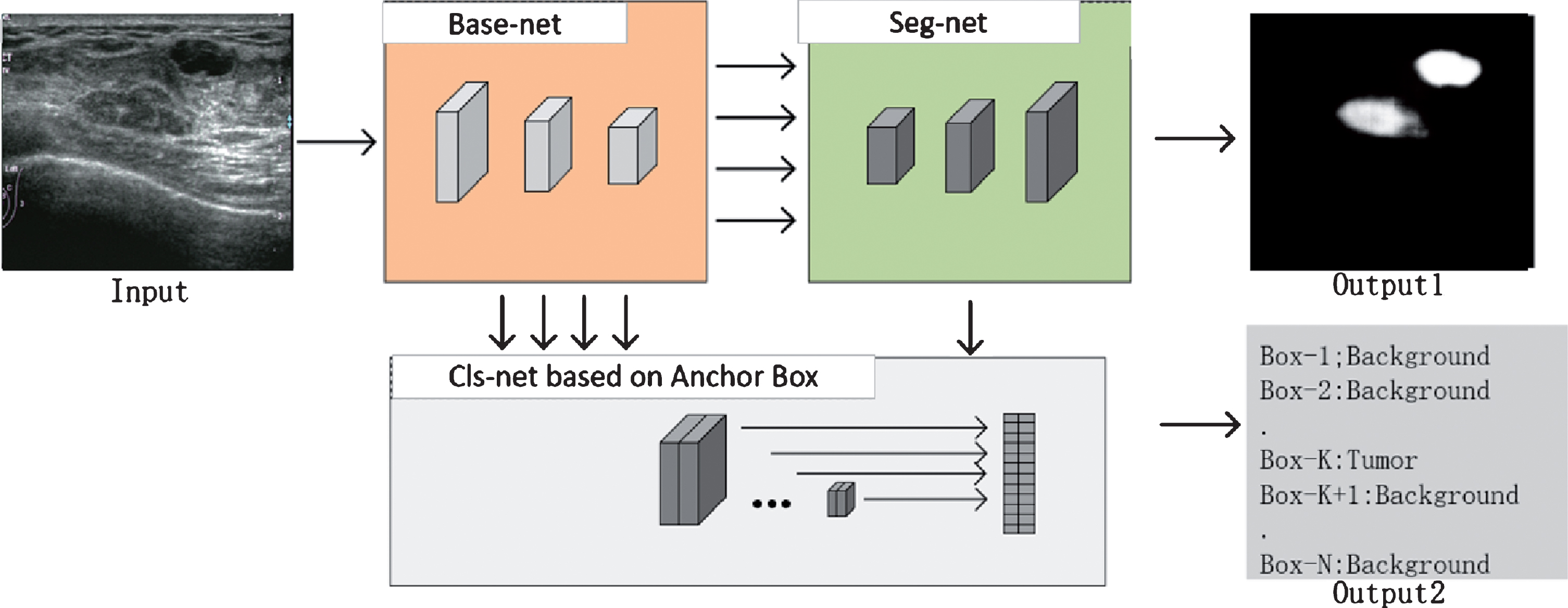
Components of the proposed single model.
The dataset was provided by the Huaxi Hospital and China-Japan Friendship Hospital, with various kinds of ultrasonic equipment, and all the sensitive information had been removed. The segmentation labels were manually outlined by professional doctors as gold standards. The dataset consists of 2280 images from different people with a mean image size of 750×650 pixels. As show in Fig. 3(a) and 3(b), the tumor size in our dataset is also diverse. Within the 2280 images, 480 were images with no lesion, 1730 with one lesion and 70 with multiple lesions. Within the 1800 lesion images, 560 images presented malignant masses (ductal carcinoma, invasive ductal carcinoma, malignant phyllode, invasive lobular carcinoma, etc) and 1240 were benign lesions (complex cyst, simple cyst, fibroadenoma, etc). Our dataset would be randomly divided into training set, validation set and test set in the cross-validation stage.

Examples of dataset: (a) Tumor sample with 38×22 mm in size. (b) Tumor sample with 3×2 mm in size.
Driven by powerful deep neural networks, pixel-level prediction like semantic segmentation and object detection tasks always choose classification model which is well trained on lager dataset like ImageNet as feature extractor. This strategy is well known as Transfer learning [26]. In this paper, as show in Fig. 4, we call the forward part of traditional classification model without linear layer as Base-net. The Base-net part of our proposed model can be replaced by most famous classification network. Many prevalent classification networks, like VGG [27], Inception v1–v4 [28–31], ResNet [32], Xception [33] and DenseNet [34], all have excellent performance on ImageNet Large-Scale Visual Recognition Challenge (ILSVRC). Different Base-net can lead to different accuracy and computation efficiency (refer to the Discussion part) which would be taken into consideration for the practical application. For example, the DenseNet, shown in Fig. 4, connects each layer to every other layer within the “Dense Block” in a feed-forward fashion, having several advantages: they alleviate the vanishing-gradient problem, strength feature propagation, encourage feature reuse and substantially reduce the number of parameters [34].
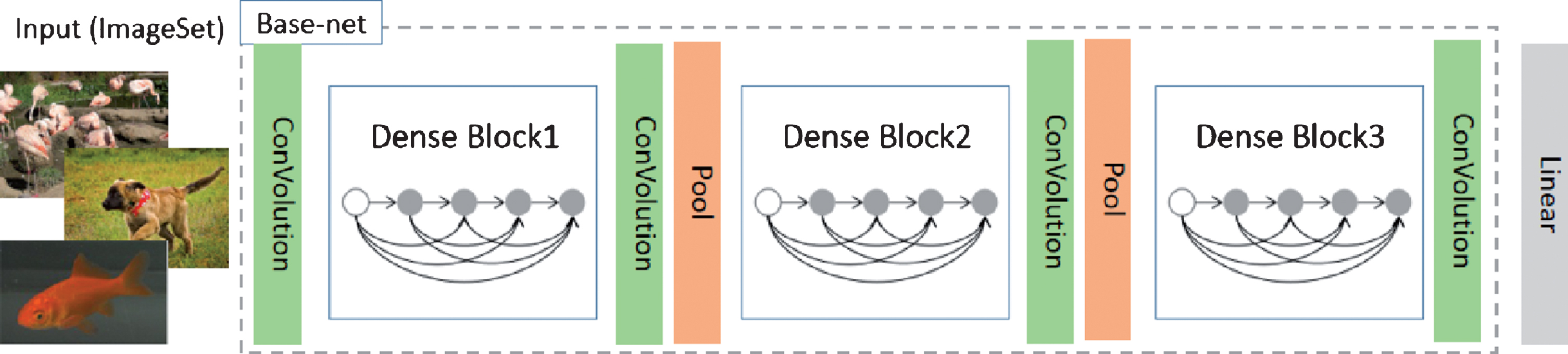
Base-net of DenseNet.
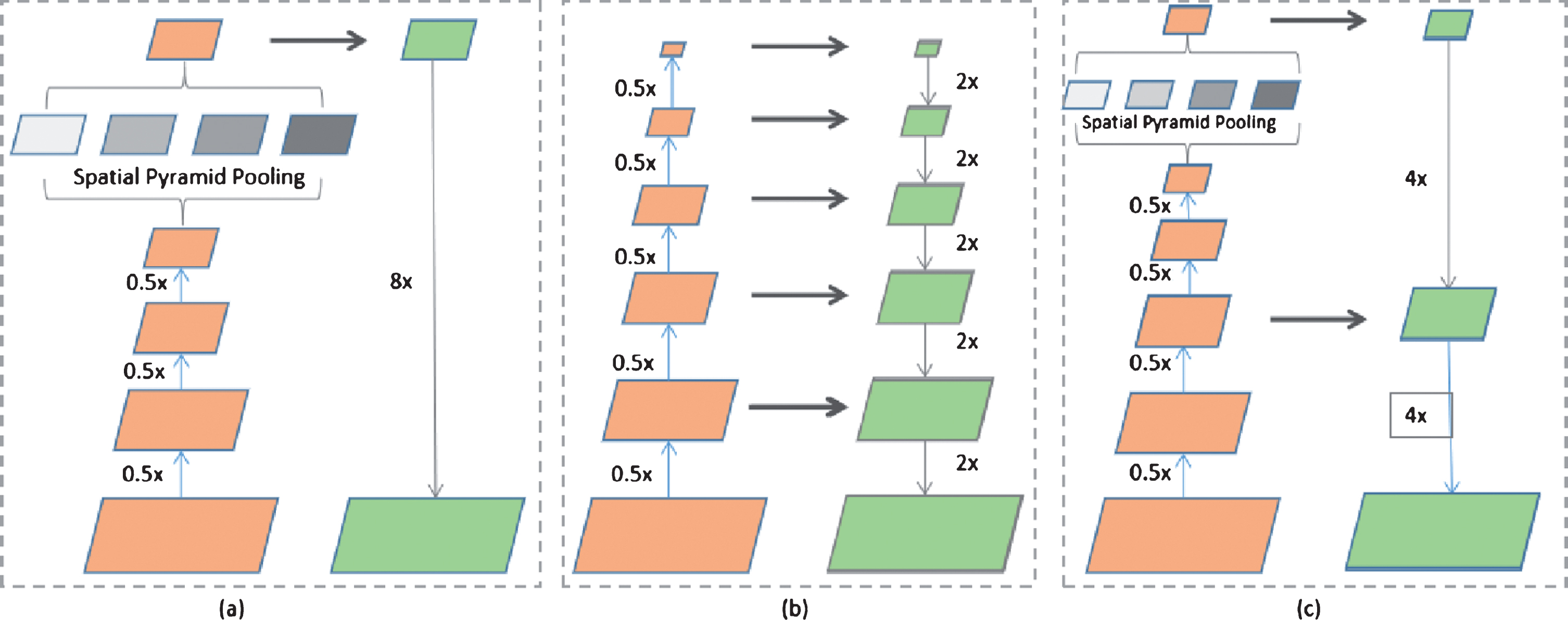
Several effective frameworks have been demonstrated considerable improvement on semantic segmentation task. As show in Fig. 5, (a) represents the framework with spatial pyramid pooling (SPP) module [35], (b) represents the framework with encoder-decoder structure and (c) represents the combination of (a) and (b). We set the decoder part or upsampling section (the right part of each frameworks in Fig. 5) of all segmentation framework as Seg-net.
Encoder-decoder framework is commonly used in the segmentation of medical image [13, 14, 16, 24]. If shallow convolution layer represents low-level visual information such as texture, color or boundary, the deep convolution layer may describe semantic feature. In Encoder-decoder structure, encoder network gets semantic features with lots of Convolution and Pooling layers and decoder network try to make pixel-wise prediction by adding Deconvolution layer. However, simply adding Deconvolution layer on semantic feature layer would lose much low-level visual features. One way to address this limitation in Encoder-decoder framework (except SegNet) is adding skip connection which fuses both deeper and shallower layers to predict sharper border. For example, RefineNet(in Fig. 6), an advanced Encoder-decoder network, makes good use of Muti-Path feature by applying three skip connections, and can get effective end-to-end training by adding lots of “Residual Conv Unit” and “Chained Residual Pooling” modules in the RefineNet Block (in Fig. 7).
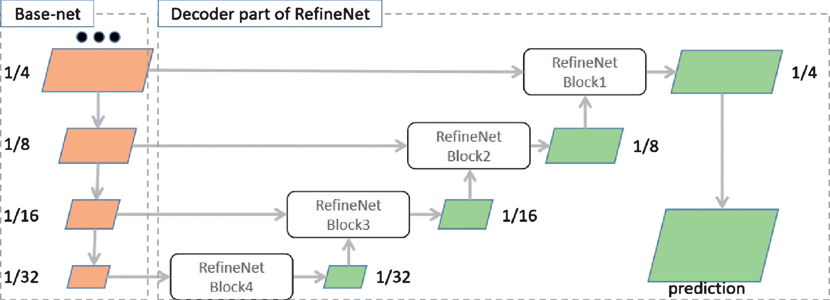
RefineNet architecture. Exploits various levels of detail at different stages of convolutions and fuses them to obtain a high-resolution prediction. The details of the RefineNet block are outlined in Fig. 7.
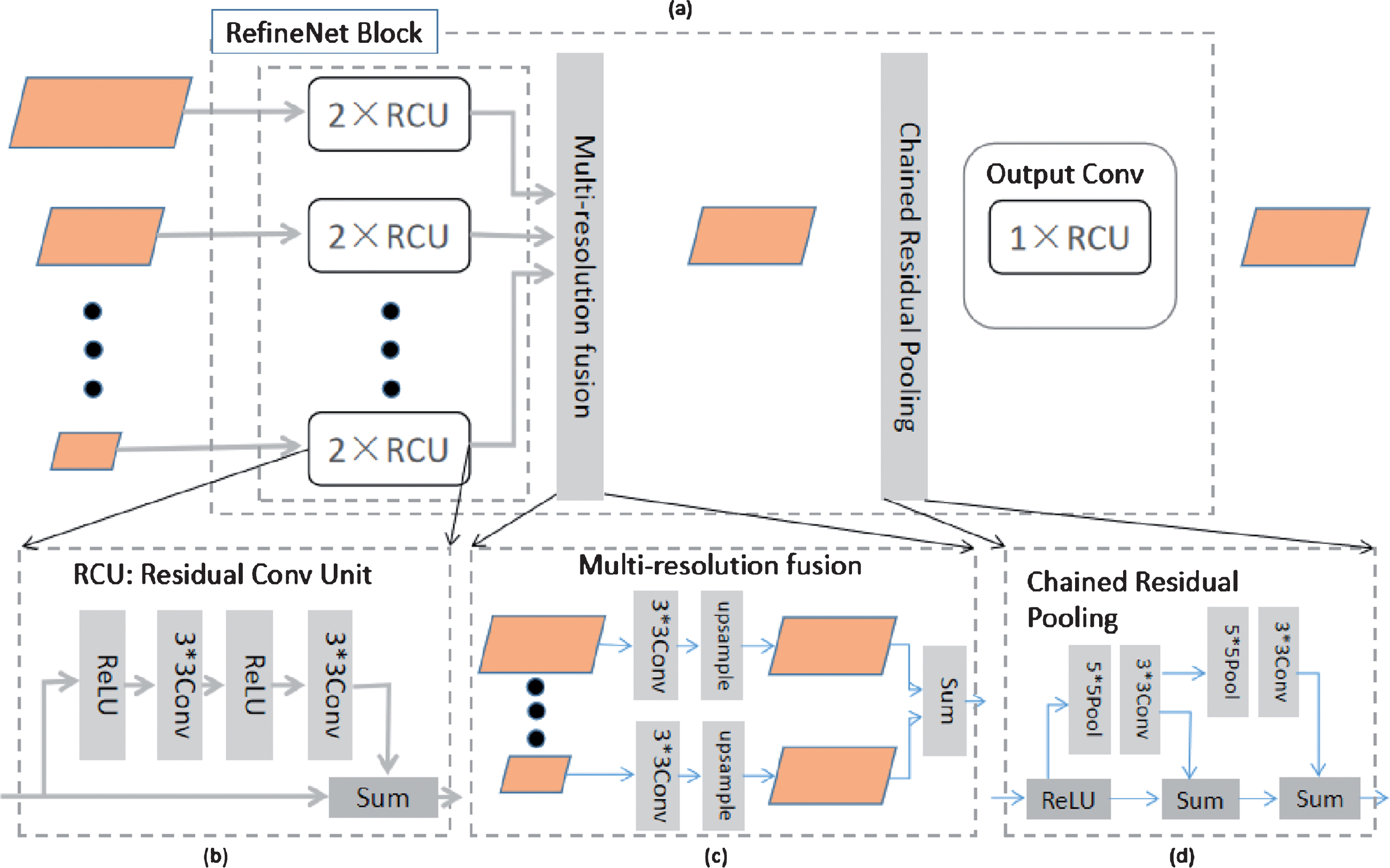
The individual components of RefineNet Block.
Anchor box
Object detection task requires predicting a collection of bounding boxes and scores for the presence of object in those boxes. Well-behaved models like Faster RCNN, YOLO and SSD all tend to apply Anchor Box to predict shape offsets and categorical confidence for all default boxes simultaneously. The detection accuracy can be greatly improved by applying Anchor Box in different size of feature layers, and various aspect ratios and scales of default bounding boxes are important for the detection of objects with different shapes [20], so SSD performs better than YOLO and Faster R-CNN on several dataset like PASCAL VOC, COCO and ILSVRC. Compared to other object detection methods, SSD also has much advantages on calculation speed.
Object detection algorithm based on Anchor Box is like a kind of sliding window model, and it can get both categorical scores and shape offset to the default bounding box coordinates for each point per feature map location. Figure 8 is a simple illustration of Anchor Box. As show in Fig. 8(a), the feature map, with size of 14*14*18, predicts bounding box (4 values) and categories (2 values) for three default boxes (different aspect ratio) every pixel of 14*14. That is, one pixel point of 14*14 need to predict 18 = 3*(4 + 2) values, so the channel of Anchor Box layer in Fig. 8(a) is 18. However, only 6 = 3*2 values were involved in our model, because our Anchor Box layer only need to output categories for each default box. Anchor box with no output of bounding box would make Cls-net be trained easily.
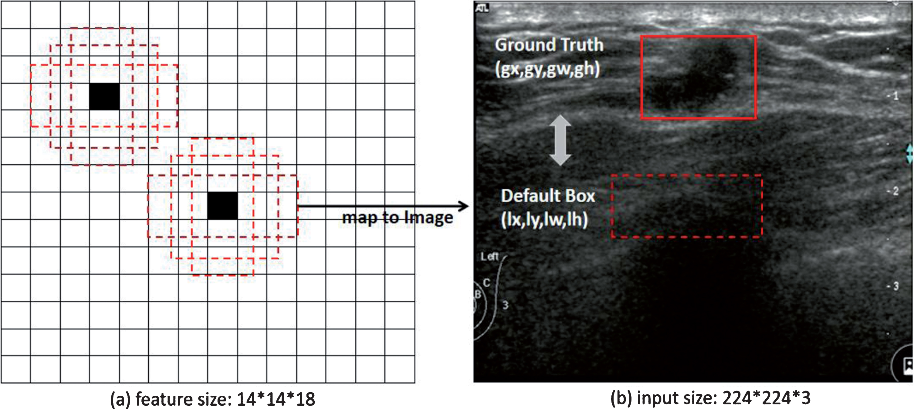
Anchor Box layer with three different aspect ratios. (a) 14*14 feature map. (b) Input image.
Motivated by anchor box and SSD algorithm, we added Cls-net (Fig. 9) on our Base-net. In Fig. 9, feature layers in Base-net with output_stride [37] = 4,8,16,32 were selected to as the inputs of our Cls-net. However, unlike SSD, features from different layers (output_stride = 4,8,16,32) were concatenated from front to back to strengthen the connection between multi-scales description. In Fig. 8, the red line also connected another layer (output_stride = 32) of Seg-net to the front section of our Cls-net, because we want to consider segmentation result with global features when detecting small tumors. What’s more, unlike SSD, prediction of bounding boxes in our model was removed, as we detected possible lesion region via Seg-net, so Cls-net only predicted categories correspond to each default bounding box which could be calculated by input size and the settings of Anchor Box layer. Similar to SSD, feature channels of AnchorConv 1,2,3,4,5 were related to the amount of classes (“nclass”) and aspect ratios of each layer which were set as Table 1. The outputs of AnchorConv 1,2,3,4,5, followed by reshaping and concatenation layer, were converted to the confidence of categories for all default boxes.
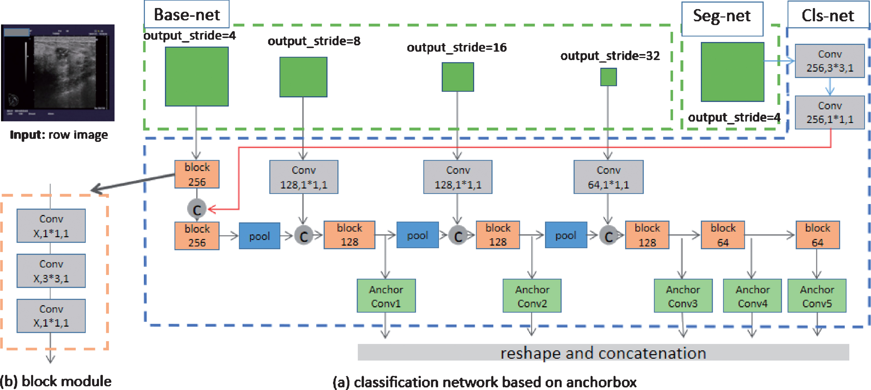
Cls-net model in this paper. (a) Classification network based on anchor box. Especially, “Conv 128,1*1,1” means Convolution layer with 128 channel, 1*1 kernel size and 1 stride. All “pool” modules in the network means “Conv n,3*3,2” where “n” is the same as former layer. All “C” modules mean Concatenation layer. (b) Block module. The block module is combined by three convolution layers, and “block 256” indicates the “x” in (b) is 256.
Aspect ratios and scales for Anchor Box layer
The settings of aspect ratio and scales for each Anchor Box layer mainly depended on the statistics of tumor size and shape in our dataset, as shown in Table 1. Similar to SSD, the Anchor Box layer with Aspect ratio = 1 represented two default bounding boxes with different scales. For example, in the first row, AnchorConv1’ Aspect ratios were set as [1.0, 1.6, 2.0], so each of them represented a default box with area = 0.08*0.08. Besides, another default box with area = 0.08*0.21 was also contained when Aspect ratio = 1.0, so the nBox was 4 = 3 + 1 and the Channel of AnchorConv1 layer was 8 = 4*2 (nBox*nclass).The outputs of AnchorConv 1,2,3,4,5 were converted to confidence of categories to all default boxes by reshaping and concatenation, and finally a two-dimensional vector with shape = (box-all, 2) could be acquired if “box-all” represented the total amount of default bounding box in the 5 Anchor Box layers.
DenseNet and RefineNet were finally chosen in our proposed model for the best accuracy (refer to the Discussion part) among those networks mentioned in 2.2 and 2.3. Our One-step model can be simply depicted as Fig. 10, where Cls-net was connected to both Base-net constructed from DenseNet and the Seg-net constructed from RefineNet. The proposed model contained two outputs, the Output1 (224*224) represented segmentation result which had the same size as input image, and Output2 (4753*2) meant there were 4753 default bounding boxes in total and 2-element vector predicted confidence of categories (tumor or background) for each default box.
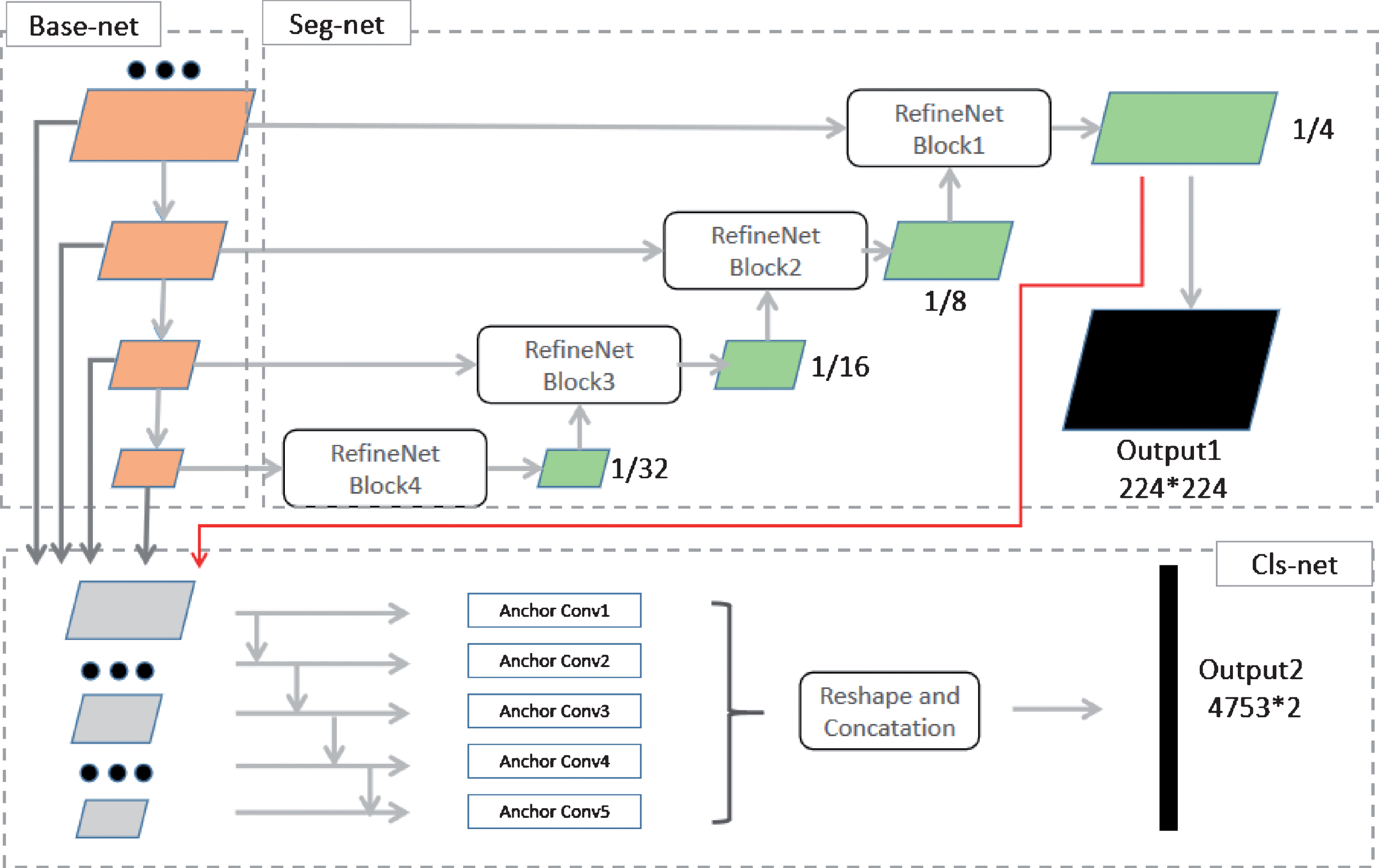
The proposed One-step model used in this study.
Extracting region of interest
After end to end and pixel to pixel training, the Outpu1 represented a probability distribution map of possible lesion region (as shown in Fig. 11(a)). We first used a threshold of 0.70 to segment the probability distribution map and reduced the threshold to 0.50 if no connected object areas acquired. We reduced the threshold by 0.20 each time until got sufficiently large connected areas, and if no appropriate object found when threshold was 0.10, it was convinced that no tumor existed in this US image. After the above operation, a set of connected components were selected and each connected component represented a possible lesion region. Finally, we got all bounding box by calculating the minimum enclosing rectangle of connected component.
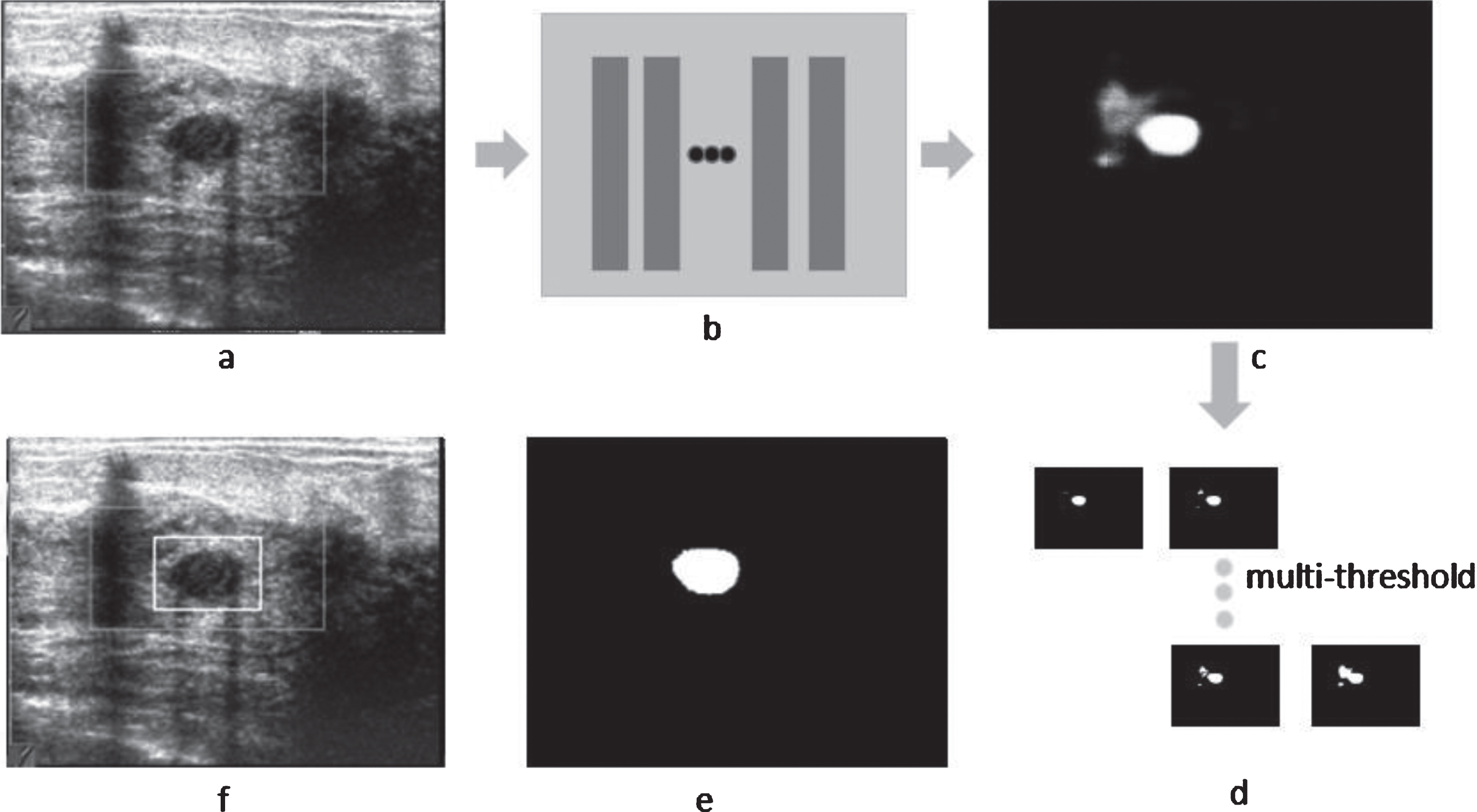
The post-processing of Output1. (a) Row US image. (b) Segmentation network (RefineNet + DenseNet201). (c) Output1: probability distribution map affected by artifacts. (d) Large probability regions are selected firstly to remove false region. (e) Region selected finally. (f) Bounding box.
A set of predicted bounding boxes about possible lesion regions were collected from Output1. Conventional methods usually crop input images according to the bounding box, and then remove false objects by applying prevalent classification networks like DensNet, ResNet or InceptionNet. However, this method has nonnegligible shortcomings. Firstly, cropping image partly would lose all global features, for the existence of tumor is strongly relevant to devices and background of image. Secondly, adding another classification network can be time-consuming and waste of memory, for all possible lesion regions need be discriminated by classification network. As shown in Fig. 12, in our method, default box and confidence predicted by Cls-net were combined together, and then by processing Non-Maximum Suppression (NMS) with 0.01 confidence threshold and 0.05 IOU threshold, a set of non-overlapping default boxes named clsbox were obtained and each clsbox corresponded to a category. Bounding boxes generated by Output1 are called selectbox in Fig. 12. Furthermore, for each bounding box in selectbox, we chosen a most closely matched one in clsbox by calculating IOU and APR, then got its confidence accordingly.
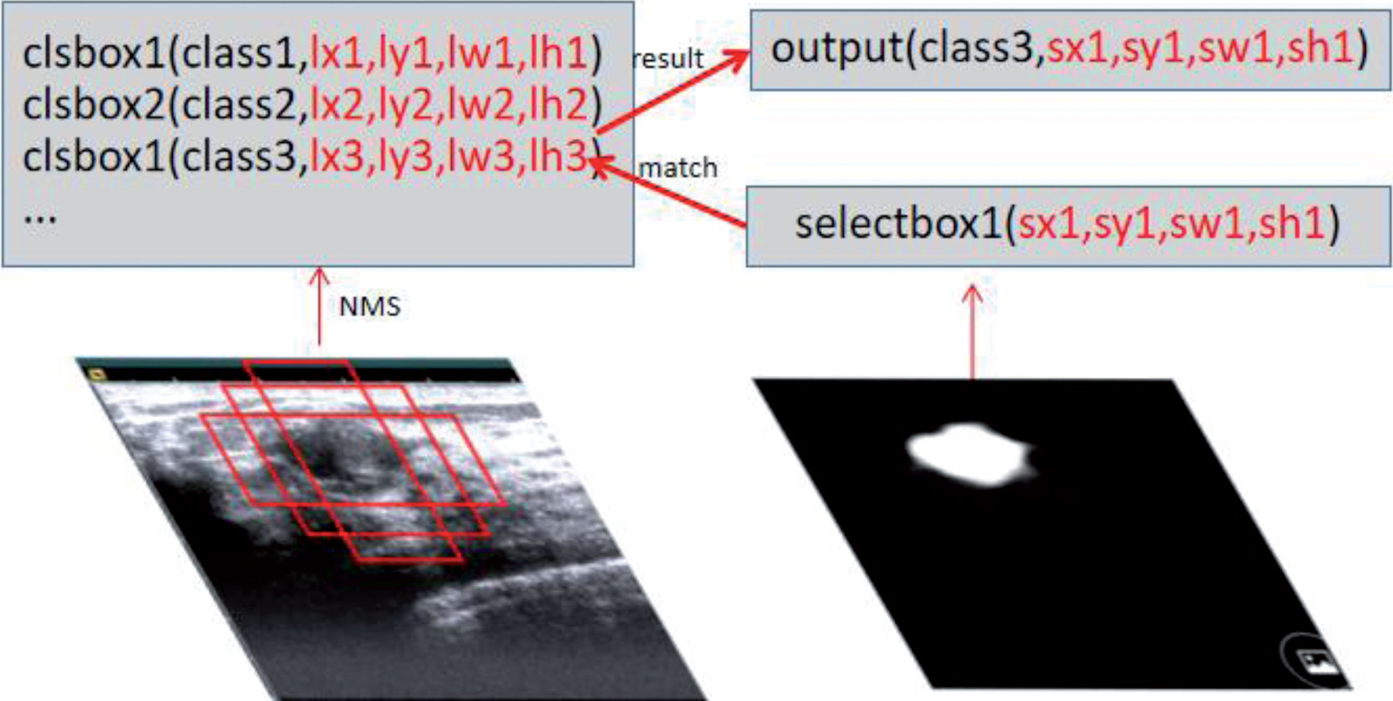
The post-processing of Output2.
Data augmentation
Labeling images for detection is far more expensive than classification, so it is respectable for our dataset containing 2280 breast US images with different devices. However, for deep learning, such dataset is still a small one, so data augmentation strategy was applied on our training process. We applied some special data augmentation strategies for low-contrast and artifacts in the US images. In addition to common data augmentation approaches like Affine Transform (translation, scale, flip, rotation), and we also adopt Gray Level Transformation(Gamma transformation, Contrast Transformation, Histogram Equalization) and added noises (random noise, Gaussian noise) on our training samples. As for training samples with multiple lesions, we also copied them several times for balancing the training data. Many studies shows Applying appropriate data augmentation can significantly improve the performance of model and make them more robust [20, 36–38, 40].
Optimization method
After simple test, we found that SGD had slow convergence rate but more stable training result. To train Base-net and Seg-net, the SGD optimization was added Nesterov momentum with updating factor 0.9. In addition, we applied “poly” learning rate policy [37] which initial learning rate was 0.02 on our training procedure. For the Cls-net, all parameters were similar to segmentation procedure except initial learning rate which was set to be 0.008.
Loss function
Binary Cross Entropy was chosen for the training of Base-net and Seg-net. For Cls-net, like SSD, we used the method of balancing tumor and background objects by 1:3 ratio while calculating the final loss each image. In SSD algorithm, the total loss was the the weighted sum of “classloss” and “locloss” which was described as follows:
Where “classloss” represents the loss of categories to each default bounding box, and “locloss” means the loss of predicted bounding box. The “w” is the weight of “locloss”, and “N” represents the number of default bounding boxes which were included in the final loss. The Anchor Box layers in our model only contained the categories to each default bounding box, so the training loss of Cls-net could be described as follows:
In this paper, our model was combined by Base-net, Seg-net and Cls-net, but they were trained separately. After Base-net and Seg-net being trained appropriately for segmentation, we then trained Cls-net network with Base-net and Seg-net fixed. The weights which were trained on the segmentation procedure would make Cls-net focus on possible lesion regions which made the second training process easier.
Evaluation metrics
Precision rate and recall rate
To compute the difference between the ground truth regions and automatically detected regions, Average Precision Rate (APR), Average Recall Rate (ARR) and F1 score were used to analyse the accuracy of bounding box like literature 22. They were defined as
Where N represents amount of all tumor objects in the test samples, R gt indicates ground truth region, and R pred indicates regions which is predicted by the proposed method.
The Stability is the evaluation of model resisted to the change of the image. After multiple measurements of the same image (each image has a certain transformation), stability can be represented by the standard deviation of the accuracy.
We applied 10-fold cross validation in the experiment. Our samples were randomly divided into 10 groups. In each experiment, we selected 1 group as the test set and 9 groups as the training set. We also selected 1/9 of training set as the validation set. We calculated the final result after repeating 10 times. The CPU of our platform was i5–6500 (3.2 GHZ) and GPU was GTX1080Ti (12G). Deep Learning Library used in our experiments was Keras with Tensorflow as back-end.
Results
To further validate the proposed fully automatic One-step model, our best combined model (RefineNet + DenseNet101 + Cls-net) was chosen to compare with SSD algorithm by calculating APR, ARR and F1 score like literature 22.
Statistical results
It has been proved that SSD outperforms other prevalent object detection algorithms like RCNN and YOLO on detection of breast US images in terms of APR, ARR and F1 score [22]. Results of literature 22 were simply quoted in the first row of Table 2 to validate our experiment/method. We also tested SSD (the input size was 300*300 and Base-net was VGG16) method with our own dataset and training methodology, and the result was shown in the second row of Table 2. The third row of Table 2 shows the result of our method without Cls-net (RefineNet + DenseNet201), and the fourth row shows the result of our proposed model (RefineNet + DenseNet201 + Cls-net).
Comparison of our method and SSD
Comparison of our method and SSD
First, as shown in Table 2, our SSD achieved lower APR but higher ARR compared with the results of literature 22 which finally led to 82.33% F1 score with our own dataset. Using different dataset and data augmentation approaches might cause the 3.38% higher F1 score on our experiment of SSD. Second, the segmentation part (RefineNet + DenseNet201) of our method achieved better result than SSD, and by applying Cls-net, our proposed One-step model (RefineNet + DenseNet201 + Cls-net) significantly outperformed SSD with 8.55% higher F1 score in our own dataset.
Figure 13 showed some samples of our experiment with no tumor existed. For Fig. 13(a), (b), our method would both detect another false region if no Cls-net applied. The misclassified regions generated by Output1 were deleted via Output2 because their confidence levels of the detected tumor were 0.30 and 0.0 (both smaller than 0.5). The objects detected by SSD in Fig. 13(b), (c) were obviously artifacts in fat layer, and Fig. 13(d) was mammary duct. Images in Fig. 13(e), (f) were difficult to discriminate because both have complex background, but our method could accurately determine that there is no tumor in these images.
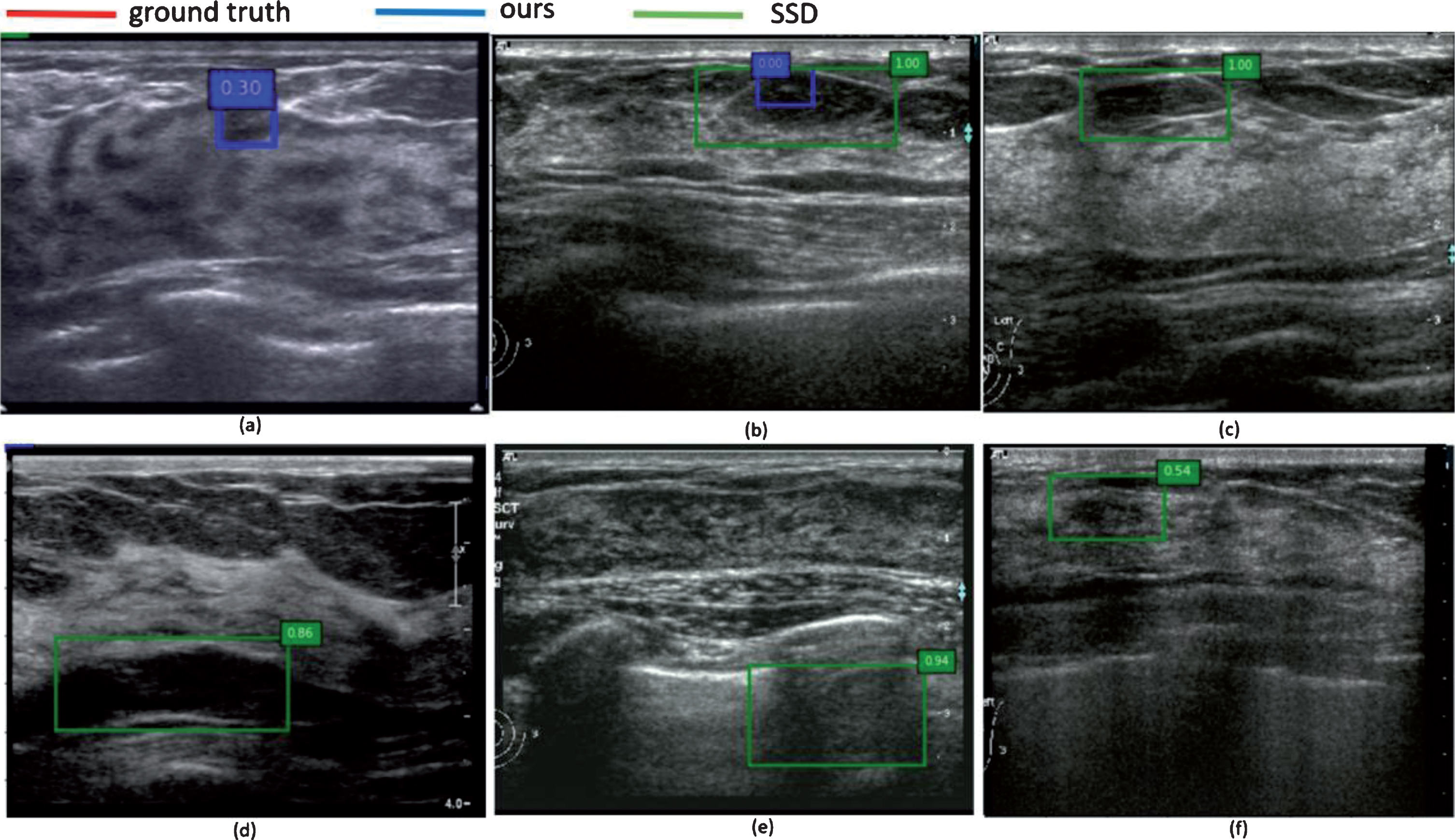
Detection results of several samples with no tumor existed.
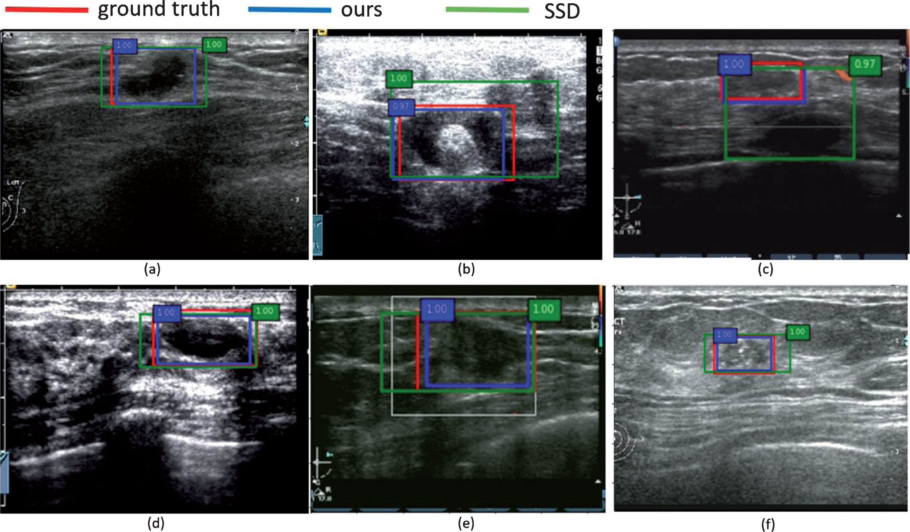
Figure 14 showed some samples of our experiment results with one or more tumors existed. Similarly, our method would detect another false object in Fig. 14(a) if no Cls-net applied. For Fig. 14(b), (c), SSD both detected another false object but not our method. More seriously, in Fig. 14(d), SSD not only detected two artifacts, but also ignored the only tumor for confidence was only 0.35. In addition, for Fig. 14(e, f), our method also successfully detected all tumors but SSD failed to detect the smallest one.

Detection results of several samples with one or more tumors existed.
In summary, it demonstrated that our proposed model has more accurate detection accuracy than SSD. On the one hand, Segmentation networks have more advantages on region proposal. The segmentation frameworks can sufficiently make full use of local features (like texture, color or boundary) and semantic feature. On the other hand, Our Cls-net only need predicting categories for each default bounding box which means Cls-net can be easily trained. Hence, although our segmentation network could detect some false regions, Our Cls-net can also remove them correctly.
Figure 15 showed some results of our experiment when it comes to the accuracy of bounding boxes. Figure 15(a) showed our method has more accurate bounding boxes than SSD on samples with clear boundary. Figure 15(b, c) were samples with artifacts around tumor objects, and bounding boxes predicted by SSD were obviously affected by artifacts but not our method. Figure 15(d, e) were samples with complicated background, our method also performed well. In addition, our method also got excellent bounding box with blurred tumor in Fig. 15(f). In summary, it demonstrated that our One-step model always has more accurate bounding boxes than SSD. One explanation is that SSD needs to remove redundant bounding boxes by using NMS algorithm like other object detection models, but the outputs of categories and bounding boxes are difficult to reach optimal training results simultaneously. Hence, the SSD would get result with high confidence of categories but poor bounding box by using NMS. However, our One-step model can avoid the problem by predicting bounding box via segmentation.
Comparison of detection results between our method and SSD.
Other famous Seg-nets (RefineNet, PSPNet and DeepLabv3+) based different Base-nets were also tested to find some rules for choosing the right Seg-net and Base-net in the practical application. Therefore, stability and time-cost were also tested for better evaluation.
Selection of segmentation framework
In the Table 3, we listed all experimental results of Seg-nets constructed from other famous segmentation frameworks. Segmentation model with only SSP module like PSPNet has the worst performance and DeepLabv3+ (with both SSP module and a single skip connection) performed better but was still not ideal. However, Encoder-decoder structures which included FCN and RefineNet had more accurate results than PSPNet and DeepLabv3+, and the RefineNet with more advanced decoder part performed best. In accordance with the above results, Encoder-decoder structures like UNet, FCN and RefineNet were the considerable choices of Seg-nets in our proposed model, and some of which are also used in other research [14, 16, 24] on medical image.
Results based on different segmentation frameworks
Results based on different segmentation frameworks
Table 4 showed the experimental results of RefineNet with various Base-nets (VGG16, VGG19, MobileNet, XceptionNet, DenseNet101 and DenseNet201). Advanced classification models like MobileNet, XceptionNet and DenseNet had more accurate results but usually costed more calculation time. It was further proved that deeper models usually had better performance which is widely accepted in classification task by comparing DenseNet101 with DenseNet201. The MobileNet might be a considerable choice of Base-net with the Consideration of accuracy and efficiency.
The results of RefineNet based on different Base-nets
The results of RefineNet based on different Base-nets
In this paper, we proposed a new One-step model which combined by Base-net, Seg-net and Cls-net based on anchor box. This strategy could get possible lesion regions with more accurate bounding box via Seg-net and remove redundant false region by Cls-net. Firstly, the experiments validated that our method significantly outperforms SSD on breast tumor detection from US image in terms of APR, ARR and F1 score. Secondly, the results demonstrated that our method also had excellently stability. Lastly, Our model achieved comparative time-cost with SSD which is the famous real time model running at 59 FPS by sharing Base-net and using smaller input size 224*224. A promising future direction is to explore its use as part of a US system by using recurrent neural networks to detect or track objects in US breast video.
Footnotes
Acknowledgements
This paper is supported by Basic Application Research Project of Sichuan Science and Technology Department (No. 2019YJ0055), the Achievement Conversion and Guidance Project of Chengdu Science and Technology Bureau (No.2017-CY02-00027-GX), and the Enterprise commissioned technology development project of Sichuan University (No.18H0832). Our images are supported by the Department of Ultrasound, China-Japan Friendship Hospital (Beijing 100029) and West China Hospital of Sichuan University (Chengdu 610000).