



Abstract
BACKGROUND:
The fusion of computer tomography and deep learning is an effective way of achieving improved image quality and artifact reduction in reconstructed images.
OBJECTIVE:
In this paper, we present two novel neural network architectures for tomographic reconstruction with reduced effects of beam hardening and electrical noise.
METHODS:
In the case of the proposed novel architectures, the image reconstruction step is located inside the neural networks, which allows the network to be trained by taking the mathematical model of the projections into account. This strong connection enables us to enhance the projection data and the reconstructed image together. We tested the two proposed models against three other methods on two datasets. The datasets contain physically correct simulated data, and they show strong signs of beam hardening and electrical noise. We also performed a numerical evaluation of the neural networks on the reconstructed images according to three error measurements and provided a scoring system of the methods derived from the three measures.
RESULTS:
The results showed the superiority of the novel architecture called TomoNet2. TomoNet2 improved the quality of the images according to the average Structural Similarity Index from 0.9372 to 0.9977 and 0.9519 to 0.9886 on the two data sets, when compared to the FBP method. This network also yielded the best results for 79.2 and 53.0 percent for the two datasets according to Peak-Signal-to-Noise-Ratio compared to the other improvement techniques.
CONCLUSIONS:
Our experimental results showed that the reconstruction step used in skip connections in deep neural networks improves the quality of the reconstructions. We are confident that our proposed method can be effectively applied to other datasets for tomographic purposes.
Introduction
Computer tomography is a well-known set of tools for the non-destructive investigation of the internal structure of an unknown object [13]. In transmission X-ray tomography the object is located between the X-ray source and the detector. This enables us to measure the attenuating characteristics of the materials of the object at the detector. The attenuation depends on the linear attenuation coefficient of the object, as the X-rays passing through the object. If the measurements are made in a lot of different directions and the geometry of the projections (i.e., the path of the beams) are known, then the reconstruction of the object under study can be made from the measured projection data [8, 13].
Our aim was to provide highly accurate methods for the case of tomography when the projection data shows strong signs of beam hardening and random electrical noise. Beam hardening is a physical phenomenon, which causes serious difficulties in tomography. Beam hardening occurs because the lower energy photons of the polychromatic radiation are absorbed with a higher probability in the material of the studied object than the higher energy photons. Therefore, if polychromatic radiation passing through an object, it will lose a greater proportion of its lower energy photons, so the ratio of higher energy photons will increase relative to the lower energy photons. As this happens, one can say that the beam becomes harder, which means that the inner layers of the object will interact with radiation having a different characteristic. Beam hardening artifacts appear in two forms such as cupping (the interior of the object appearing to be darker) and dark or light streaks (see Figure 2). Electrical noise is a random factor in the measurement process causing random changes of the measured values. In the reconstruction, it causes streaks and random changes in the pixel values.
In order to cope with these measurement errors, we created a database with a virtual CT scanner, producing realistic simulations of projection data and we designed two novel deep-learning based methods for reducing artifacts in the reconstructions.
One of the sub-fields of artificial intelligence, called deep learning [14], has achieved outstandingly good result in the field of computer vision and digital image processing in the last decade. When using deep neural networks, the word “deep” means that the network structure contains multiple hidden layers [23]. In this paper, we used an outstandingly versatile and useful tool of deep learning called U-net [22].
The literature provides a variety of options (e.g., in [24]) for the combination of computer tomography and deep learning methods. There are approaches for the reduction of various artifacts, for example beam hardening [7, 20] and metal artifact [4, 28]. Moreover, researchers in [3, 26] were interested in performing the reconstruction with neural networks, while others applied deep learning as a pre- or post-processing tools before- or after the reconstruction in [2, 17].
In this paper, we present two novel deep convolutional neural network architectures for image reconstruction from projections. These methods provide end-to-end solutions taking projection data as an input and producing reconstructed images on their outputs. In comparison, the end-to-end solution in [26] has simpler architecture than ours and also it contains a fully connected layer. The end-to-end reconstruction architecture in [3] has a more complicated architecture with three well-separated parts. The first part is working on the projection data with convolution layers. The second part performs the reconstruction, while the third part is working on the reconstructed images with convolution and deconvolution layers. This method maintains a weak connection between the parts working with the projection data and the reconstructed images. Our methods were built on the U-net structure by incorporating the reconstruction in the skip connections. In this way, the reconstruction is not before, or after the main part of the network, but in the middle of a U-net structure, thus the connection is stronger, which makes the training easier, and more efficient.
This paper is structured as follows. In Section 2 we formulate a model for tomographic reconstruction that we used, with providing the most important equations. Next, we describe the evaluation datasets in Section 3 and the architectures in Section 4. After that, we detail the training process of the neural networks in Section 5 and present our result in Section 6. Finally, we summarise the main points in Section 7 and make conclusions in Section 8.
Computer tomography
Let
Practically, the object of study is located between the X-ray source (S) and the detector (D), resulting in a limited span of f. Therefore, the range to be integrated can be simplified to the [S, D] interval in (1). The I
D
and I
S
values are measured by CT scanners, where I
D
is the number of X-ray photons sensed by the detector and I
S
corresponds to the number of photons leaving the source. The relation between I
D
, I
S
and (1) is given by the Beer-Lambert law as
A common algorithm for creating reconstructions from projections is the Filtered Back Projection (FBP) [13]. The FBP algorithm contains a filtering step traditionally in the Fourier domain. There are a couple of well examined basic filters in the literature [8]. In Section 6 we shared our results using different filters in the FBP algorithm, which table helped us decide, what kind of FBP filter to use in the final comparison if the reconstruction step located outside of the neural network.
The FBP is fast and can give images of good quality but requires a high number of projections. The FBP algorithm was not designed to deal with the difficulties caused by physical phenomena such as beam-hardening (i.e., it assumes perfect measurements), therefore it creates various artifacts on the reconstructed image if it is supplied with distorted projection data.
We used computer-simulated artificial data in this study, generating the projections of software phantoms. Our physically correct projection data was generated using the GATE software [10, 11] without Compton scattering. We have set a parallel beam geometry and photon-counting detectors in the GATE model. 400 000 photons left the source in each projection angle. The projection data were generated with 596 angles each containing 362 detector points. The projection data was reconstructed as 256x256 images.
We have split our versatile dataset into two big parts, that we call Dataset A and B, in order to get a simple notation. For more convenient discussion, from this point on, we will be mentioning these two groups of data as different datasets. The two datasets are different in the shape and material composition of the phantom object.
Dataset A
In the case of Dataset A, we used five different X-ray sources assigned in equal proportions to 5 000 phantoms to be more realistic. We used pre-filtering during the generation of source characteristics as it is a common way to reduce beam hardening [12]. The characteristics of the sources were calculated by [21]. The sources differ only in the thickness of a pre-hardening aluminum filter. Figure 1 shows the characteristic of the sources. Each phantom was present in the dataset using only one selected source. In addition, we calculated the images of Figure 2 showing an example for all of the used sources with one phantom, which way the effect of the different sources is more visible. Figure 3 shows the intensity value profiles along the yellow lines in Figure 2. As one can see, the effects of beam hardening are decreasing towards the wider aluminum filters, while the electrical noise is increasing.

The characteristics of the X-ray sources with different aluminum thicknesses used in our experiments.

The ground truth phantom and its reconstructions from distorted projection data acquired using different pre-hardening filters.

Intensity value profiles along the yellow lines in Figure 2.
The phantoms were generated as a combination of randomly chosen shapes, i.e., circles, ellipses, and rectangles. The objects may contain each other but partial overlap was not allowed. One object can consist of only one material from the following set: air, spine bone, rib bone, skull, blood, cartilage, kidney, kidney stone, and adipose. Moreover, the objects are various in size and location, which parameters were chosen randomly during phantom generation. The phantoms were generated in 4 groups based on their object counts. Each group contained a quarter of all the images (i.e., 1250 images), and groups were generated with a maximal object count of 4, 5, 6, or 7 objects. Figure 4 introduces a few examples from this dataset.

Examples from the Dataset A.
For a ground truth projection set of the Dataset A, we calculated analytically correct projections with the help of [27] without any noise. We set the values of the materials to their mass linear attenuation coefficient. To this end, we performed specific GATE measurements, where the quotient of the detector intensity behind the object and the source intensity (in other words, the transmission value) were in the [0.4995 ; 0.5005] interval. After the measurements, we calculated the linear attenuation coefficient of the materials for each X-ray source based on (2) which was divided by the density of the material.
Before training, we applied (2) to the projection data. Then, we normalized the intensities to be in the [0, 1] interval. We used five different scaling factors corresponding to the five sources.
A second dataset was produced using hand-drawn shapes as templates from [1] with the same simulation method as Dataset A. This dataset was excluded from training and was only used in the testing of the methods. Figure 5 introduces a few examples from this data set, which consists of 66 phantoms with various non-basic geometrical shapes. Results were generated with the source pre-filtered by 5 mm aluminum. The 66 icon phantoms can be partitioned into three groups with 22 phantoms in each group. The object or objects of the phantoms in the first group (I) consist of rib bone while the background is always air. The material of the objects in the second group (II) can be air, spine bone, rib bone, skull, blood or adipose, while air, adipose, teeth, skull, ribs spongiosa or rib bone in the case third group (III). This means, that in the third group there are two materials (teeth and ribs spongiosa), which were not used during the training of the networks. In each group, random cracks were created and every phantom appears with and without the cracks. The cracks consist of air. Here, we also performed normalization with a distinct scaling factor in each group. The dimensions of the projection data and reconstructed images were the same as with Dataset A.

Examples from the Dataset B.
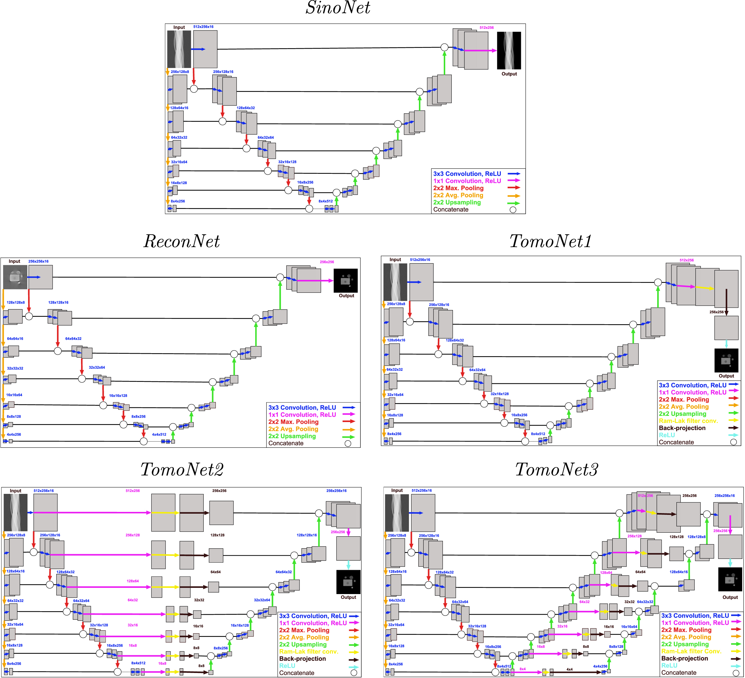
We examined the merits of our two novel architectures called TomoNet2 and TomoNet3 is this study. All of these networks are based on the special deep-, fully-convolutional neural network structure called U-net [22]. The structures of the networks are shown in Fig. 6.
The structures of the used deep convolutional neural networks.
The structure of the SinoNet and the ReconNet are the simplest ones. They have a U-shape consisting of the contracting path (left side) and the expansive path (right side) and they also have an additional average pooling connection which is concatenated to the contracting path. The difference between SinoNet and ReconNet are the inputs and outputs. The SinoNet is working on only the projection data. The reconstruction step can be carried out as an additional step after processing the projection data. The usage of ReconNet, on the other hand, takes place after the reconstruction as a post-processing step. Results using only projection data or reconstructed images in a U-net-like structure can be found in [2, 19] and [5, 20] respectively.
The TomoNet1 starts with the SinoNet structure, but the authors added new elements corresponding to the FBP. The new elements are similar to the construct in [6, 26] and exactly the same as FBP_U_net in [18]. The first element is a convolution with a Ram-Lak filter in projection space. The inverse Radon transform is the differentiable second element, which is part of the training as a neural network layer. The first and second part contains non-trainable parameters. The third element is a ReLU activation layer. The network prefers the positive values with the ReLU, which is optimal for the reconstruction tasks. The TomoNet1 accepts projection data as input and provides reconstructed images as output. The main novelty of this network was that the reconstruction and the network did not separate processing steps. The Network contains the FBP as a differentiable layer, so the training process includes the effects of the FBP.
In the case of TomoNet2, we mixed the SinoNet, ReconNet and TomoNet1 in a well-organized structure. The three elements correspond to the FBP located between the contracting and expansive paths in every level of the U-shape. Accordingly, the projection data of the contracting path transformed to reconstructed images at the expansive path. The TomoNet2 uses projection data as input and provides reconstructed images as output.
The TomoNet3 uses projection data as input and provides reconstructed images as output too, but here the contracting path and the expansive path of the U-shape are operating with projection data. Nevertheless, the FBP is present at every level forming a new expansive path.
The training was performed on an NVIDIA GeForce RTX 2080 GPU using CUDA 10.1 and cuDNN v7. We used the TensorFlow Keras library running on Python v3.6. We used only Dataset A for training and validation. We have split the 5 000 images of Dataset A into three partitions, namely, train, validation and test. The proportions were 70%, 20%, and 10% respectively. The presented results were made with the same split, but shuffle was allowed among epochs during training and validation. An additional test was done using the phantoms of Dataset B, in which phantoms remained unseen during training and validation.
We trained the networks several times with different hyper parameters and we chose the final settings leading to the best reconstruction quality. These settings are summarised in Table 1. We applied early stopping, which stopped the training if the validation loss stopped decreasing for twenty epoch and resets the network snapshot that resulted in less validation performance. In this way, we completely excluded the compromising effect of overfitting from our results.
Hyperparameters of the deep convolutional neural networks
Hyperparameters of the deep convolutional neural networks
The loss and validation function diagrams of all the networks can be seen in Figure 7. We marked (with a red arrow) the best state, which was saved by the early stopping. The loss and validation loss of the models decreased rapidly during the first few epochs, then they moved slowly toward the zero line. We considered the curves satisfactory in all respects. Although, the curves of loss and validation loss functions moved away from each other before the stopping point in the case of ReconNet.
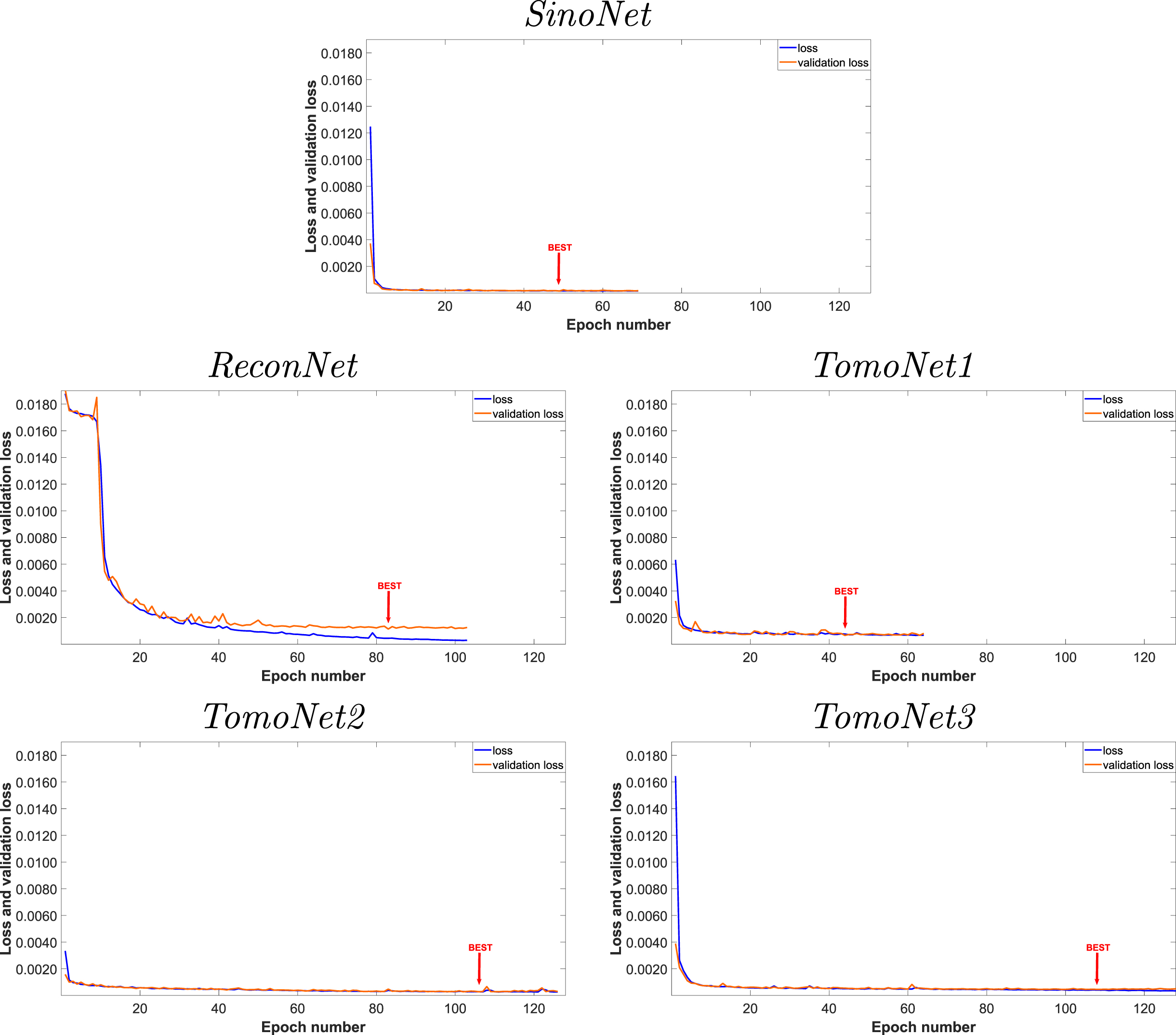
The normalized loss and the validation loss values of the deep neural networks during the training phase. The red arrows mark the best learning state of the networks, which were used for prediction.
We evaluated the reconstructed images by numerical measurements. During the evaluation, we used the Mean-Squared Error (MSE), the Peak-Signal-to-Noise-Ratio (PSNR) and the Structural Similarity Index (SSIM) [25]. All of these measurements compare the reconstructed image to the ground truth. The (SSIM) is originally limited to the (-1, 1] interval, but we considered complementary similarity as errors, therefore, negative values were replaced by zeroes. In this composition better results are marked with a higher PSNR value, an SSIM value closer to one and a MSE value closer to zero.
We compared the networks to each other and we also included an FBP algorithm (referred as (FBP) in the figures) using the Han filter. We chose the Han filter based on a test on Dataset A examining the Ram-Lak, Shepp-Logen, Cosine, Hamming, and Hann filters. Table 2 shows the results of the test. Clearly, the performance of the Han filter seems to be the best, therefore we included only the columns of the Han filter in the upcoming tables.
Calculated mean and standard deviation (SD) values for all tested imaged according to Dataset A by categories with three error types. The first column corresponds to the five sources having pre-hardening aluminum filters of different thicknesses (i.e. the categories). The last row of the first column shows the overall average. The columns of Ram-Lak, Shepp-Logen, Cosine, Hamming and Hann corresponds of the five most common filter used in FBP
Calculated mean and standard deviation (SD) values for all tested imaged according to Dataset A by categories with three error types. The first column corresponds to the five sources having pre-hardening aluminum filters of different thicknesses (i.e. the categories). The last row of the first column shows the overall average. The columns of Ram-Lak, Shepp-Logen, Cosine, Hamming and Hann corresponds of the five most common filter used in FBP
Table 3 and Table 4 show the average results of the methods with Dataset A and B by category. In the case of Dataset A, the categories correspond to the used sources. In Table 4 the category I denotes the phantoms with two intensities (background is air and object is rib bone). The phantoms belonging to row II contain four to six materials, which were seen by the networks during training. In the phantoms of category III the number of different materials can vary between four and six, from which two have not been seen by the networks during training. In addition, we calculated the overall average in both tables and provided the standard deviation of each category.
Calculated mean and standard deviation (SD) values for all tested imaged according to Dataset A by categories. The first column corresponds to the five sources having pre-hardening aluminum filters of different thicknesses (i.e. the categories). The last row of the first column shows the overall average
Calculated mean and standard deviation values for all tested imaged according to Dataset B by categories. The category I contains phantoms with two intensities. The phantoms belonging to the category of II can be constructed only of known materials showed to the networks during training. The phantoms of III contain at least one material unseen of the networks during training. The last row of the first column shows the overall average
Comparing to the basic FBP, all of the networks improved the quality of the reconstructed images according to the average measurements in Table 3. Moreover, Table 3 and Table 4 shows, that TomoNet2 outperformed the others, but it was followed closely by TomoNet3.
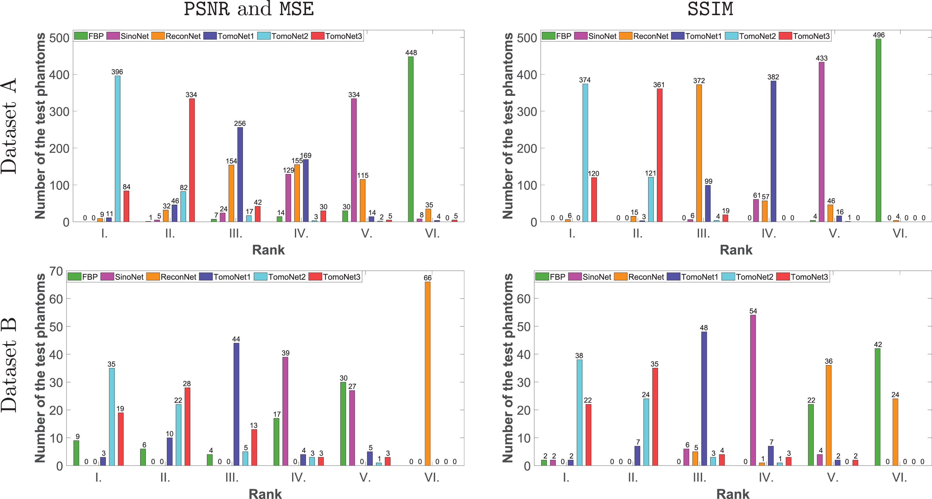
For a better insight, we summed up, how many 1st, 2nd, 3rd, 4th, 5th and 6th best places were achieved by the networks. In this manner, 1st place means that the given network gave the best result. Figure 8 shows detailed statistics about this ranking.
The achieved ranks by the networks by all of the measured errors.
In the case of Dataset A, we observed clear dominance in favor of the TomoNet2 looking at Figure 8. TomoNet2 gave the best in 396 cases according to PSNR and MSE and in 374 based on SSIM out of the 500 test phantoms preserved for testing. This means, that the TomoNet2 out-performed the other methods certainly in 74.8 percent of the cases, but we argue that it is closer to 79.2 based on PSNR and MSE. This ranking corresponds to the results seen in Table 3, which shows the dominance of one of our proposed methods in each category.
In the case of Dataset B, we can say, that TomoNet2 had the best performance with all error measurements looking at Figure 8. Note, that ReconNet only made the reconstruction worse looking at the PSNR and MSE diagram.
Table 5 shows the total score of the networks for all errors. The total score was calculated by the formula
The total rank weighted score gained by the methods for all errors. The smaller is better
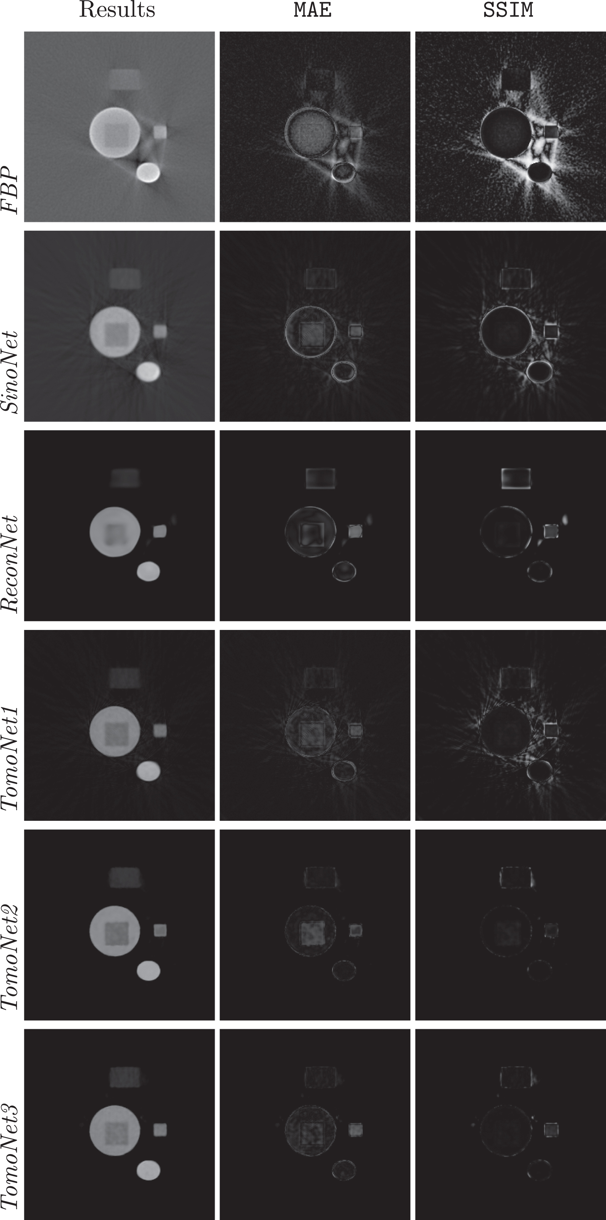
Figure 9 and Figure 11 present examples from datasets A and B. The FBP reconstruction shows strong signs of beam hardening artifacts and electrical noise with the FBP in Figure 9. The errors have been highlighted by the
Results,

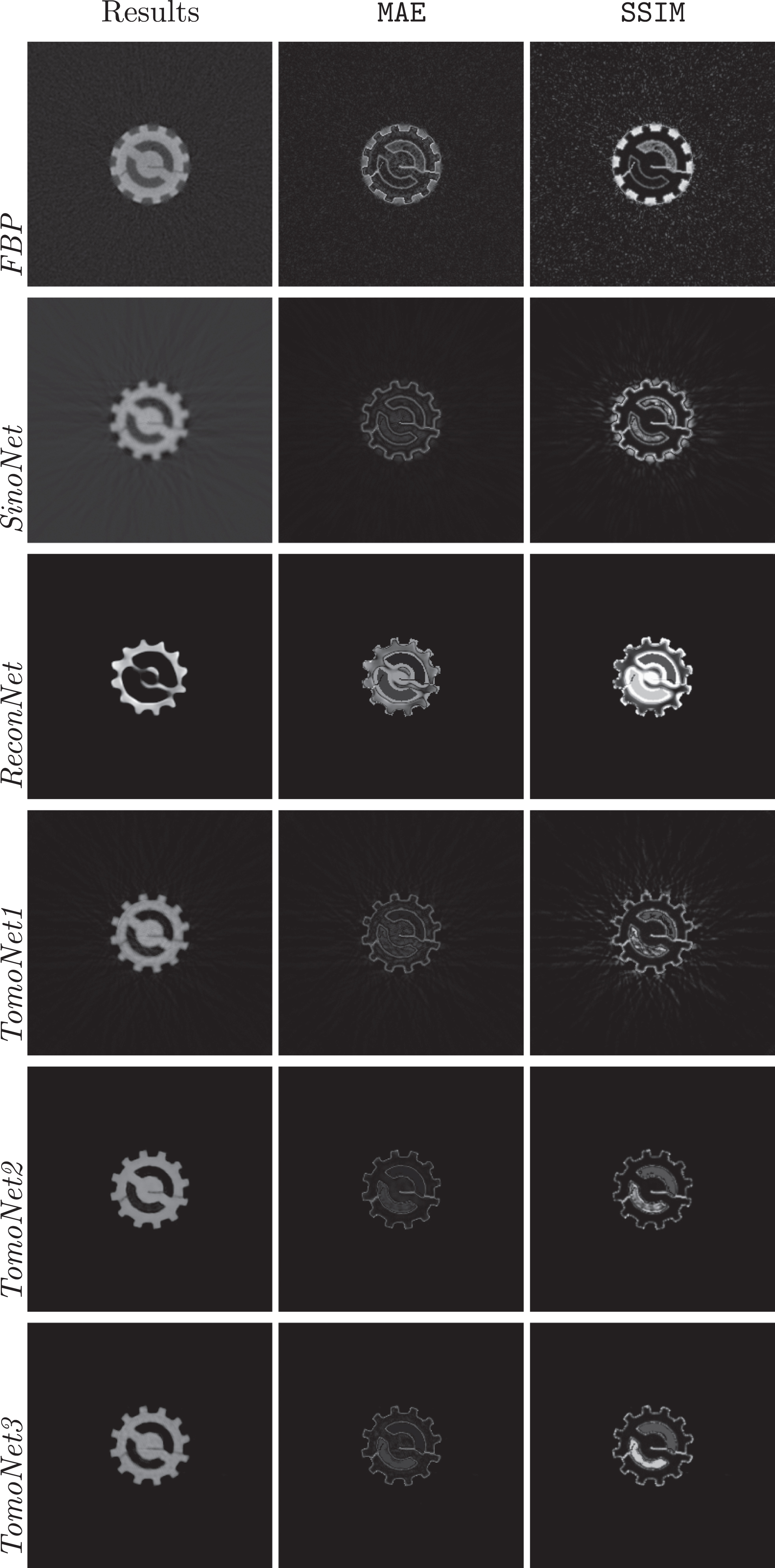
Results,
The reconstruction in Figure 11 also shows signs of beam hardening artifacts and electrical noise with the FBP. This phantom is from the “two unseen materials” category and it also contains three cracks. Here again, ReconNet was struggling to keep the shape of the objects and as a result, it gave back an amorphous form. SinoNet yielded a decent result but left some streak artifact on the image. The results of TomoNet1 and TomoNet3 are blurry, but the cracks are all along recognizable especially with TomoNet1. The reconstructed images are sharper according to the results of TomoNet2, and the surrounding low-intensity object is better preserved. However, the cracks have disappeared in some places.
In this paper, we proposed two novel neural networks for image reconstruction from projections. The novelty of the network is that they contain multiple back-projection layers, which provide a strong connection among the two main parts of the network working on projection data and working on reconstructed images, respectively.
In the literature, there are many publications that use deep learning techniques combined with tomography. But these solutions operate mainly as pre- or post-processing steps added before or after the reconstruction. Looking at our results it is clear, that the end-to-end solutions yielded better results. In our opinion, the reason for the superiority of the new models is, that if the network sees the whole path of the data, then it can better optimize the output and learn more complex features.
The authors in [6] has already demonstrated, that the FBP can be mapped into a neural network. But the authors did not intend two solve common tomographic problems like beam-hardening in this study. The authors in [3] modified the previous network to be more general and created the ADAPTIVE-NET. In their paper, there is an exhausting study about the ADAPTIVE-NET and its variants. The ADAPTIVE-NET is made up of three parts: a Projection domain unit, a Domain transformation unit, and an Image domain unit. The Domain transformation unit is responsible for the image reconstruction and the connection of the other two parts. In comparison, the base of our proposed networks is a modified U-net, where the reconstruction is performed on the skip connections. This means, that if we would divide our proposed networks into Projection domain unit and Image domain unit using the names in [3], then we had multiple Domain transformation units among them.
Here we list our five major observations based on the Section 6 to highlight the merits of our proposed methods: In our opinion the stronger connection among the domains is crucial for a more general solution, which can work with our raw projection data affected with strong distortions. We also argue that the methods improved the image quality regardless of the used pre-filtering according to Table 3, although the highest improvement was detected in the case of the 5 mm aluminum filter. The ranking analysis revealed, that the networks and the averages are reliable because there is a clearly dominant network in each place. This means, that there is a network in every given place, which ends up at the given place more than 50% of the cases. Only ReconNet made an exception in the case of Dataset A with PSNR and MSE, because its ranks are spread out over the rankings (i.e., 3-th place in 30.8%, 4-th place in 31%, 5-th place in 23%). Testing the networks against “unknown shapes” (i.e. shapes not present when training the networks) in Dataset B definitely caused a drop in the performance of all networks. Especially for the ReconNet, in which PSNR and MSE values became worse as if we had not done anything (i.e. FBP). As a reminder, we did not use the phantoms of Dataset B during training, therefore we concluded, that the ReconNet strongly relies on shape priors and it could not learn the patterns general enough to be able to gain good results on the unseen phantoms of Dataset B. The introduction of new materials caused no problem. All methods handled the phantoms with unseen material well – according to the minor difference between the category of ”II” and ”III” in Table 4.
Conclusion
In this paper, we presented two novel deep convolutional neural network architectures (TomoNet2 and TomoNet3). These methods outperformed previously existing approaches on our heterogeneous data sets, in which datasets were exposed to beam hardening artifacts and a high amount of electrical noise. Our experimental results showed that the reconstruction step used as an inner part of the deep neural networks improves the quality of the reconstructions when the projections are affected by beam hardening. The SinoNet and ReconNet are not attached to the reconstruction, while in the case of TomoNet1 the connection is weaker than with TomoNet2 and TomoNet3. We are confident, that both the TomoNet2 and TomoNet3 will be useful on other datasets for tomographic purposes.
As an improvement, we are interested in replacing the non-trainable Ram-Lak filter with a trainable one in the future. Moreover, we are working on a more effective loss function, while also implementing the TomoNet2 and TomoNet3 networks using fan-beam geometry. We are also planning to make our dataset available online.
In addition, we are currently working on the acquisition of real data. We expect, that the proposed algorithms will operate well on industrial data with some adjustments. On the other hand, we may need to implement changes for instance using fan-beam geometry and expanding the training dataset for applications on clinical data.
Footnotes
Acknowledgments
This research was supported by grant TUDFO/47138-1/2019-ITM of the Ministry for Innovation and Technology, Hungary.
This research was supported by the project “Integrated program for training new generation of scientists in the fields of computer science”, no. EFOP-3.6.3-VEKOP16-2017-00002.
This research was supported by the projects “Extending the activities of the HU-MATHS-IN Hungarian Industrial and Innovation Mathematical Service Network” EFOP-3.6.2-16-2017-00015.