An Advanced Approach to Extraction of Colour Texture Features Based on GLCM

Abstract

This paper discusses research in the area of texture image classification. More specifically, the combination of texture and colour features is researched. The principle objective is to create a robust descriptor for the extraction of colour texture features. The principles of two well-known methods for grey-level texture feature extraction, namely GLCM (grey-level co-occurrence matrix) and Gabor filters, are used in experiments. For the texture classification, the support vector machine is used. In the first approach, the methods are applied in separate channels in the colour image. The experimental results show the huge growth of precision for colour texture retrieval by GLCM. Therefore, the GLCM is modified for extracting probability matrices directly from the colour image. The method for 13 directions neighbourhood system is proposed and formulas for probability matrices computation are presented. The proposed method is called CLCM (colour-level co-occurrence matrices) and experimental results show that it is a powerful method for colour texture classification.

Keywords

Co-occurrence Matrices Feature Extraction GLCM Image Texture Analysis

1. Introduction

In recent years, the need for efficient content-based image retrieval has increased tremendously in many application areas, such as biomedicine [1,2], military [3], commerce, education, and web image classification and retrieval [4 –6]. Currently, rapid and effective image retrieval from a large-scale image database is becoming an important and challenging research topic [7]. One of the most popular fundamental research areas is content-based image retrieval (CBIR) [8 –10].

Although CBIR has been a very active research area since the 1990s, there are still a number of challenging issues due to the complexity of image data. These issues are related to long-standing challenges among several interdisciplinary research areas, such as computer vision, image processing, image database, machine learning, etc. In a typical CBIR, image retrieval is based on visual content such as colour, shape, texture, etc. [8 –10].

Texture has been one of the most popular features in image retrieval [11]. Even though greyscale textures provide enough information to solve many tasks, the colour information was not utilized. But in recent years, many researchers have begun to take colour information into consideration [12 –17].

The human eye perceives an image as a combination of primary parts (colour, texture, shape). Therefore, our approach is oriented to creating robust low-level descriptors by a combination of these primary parts of the image. Specifically, research on the combination of colour and texture is presented in this paper.

The outline of the paper is as follows. In the next section, an overview of basic principles of GLCM (grey-level co-occurrence matrix) and Gabor filters, and the extraction of colour features based on these methods are introduced. The novel method called CLCM is presented in section 3. In section 4, the texture classification and evaluation methods are described. The experimental results are presented in section 5. Finally, a brief summary is presented in section 6.

2. Related Work

There are several approaches to how colour and texture can be combined. Ye Mei and Androutsos [13] introduced a new colour and texture retrieval method, based on wavelet decomposition of colour and texture images on the hue/saturation plane. Assefaa et al. [14] discussed how the spectral analysis of each colour component of an image leaves us without information about the coupled spectra of all colour components. They introduced the idea of computing the Fourier transform of colour images as one quantity. Jae-Young Choi at al. [16] proposed new colour local texture features (colour local Gabor wavelets and colour local binary pattern) for the purpose of face recognition. Hossain and Parekh [17] extended GLCM to including the colour information for texture recognition by separating colour channels' combinations, e.g., rr, gg, bb, rg, rb, gr, gb, br, bg. In our previous work [18], new possibilities to improve the GLCM-based methods were presented. In this paper, new and extended experiments with GLCM are described and novel methods are proposed.

3. Grey-level methods

3.1. Grey-level co-occurrence matrix

The GLCM (grey-level co-occurrence matrix) is a powerful method in statistical image analysis [19 –22]. This method is used to estimate image properties related to second-order statistics by considering the relation between two neighbouring pixels in one offset as the second order texture, where the first pixel is called the reference and the second, the neighbour pixel. GLCM is defined as a two-dimensional matrix of joint probabilities between pairs of pixels, separated by a distance d in a given direction θ [19–20].

For the scale invariant of the texture pattern, the GLCM is standardized by total pairs of pixels as follows:

p_{d, θ} (i, j) = \frac{P_{d, θ} (i, j)}{A l l_p a i r_o f_p i x e l s},

(1)

where P_d,θ(i,j) expresses joint probabilities between pairs in distance d and direction θ, and i, j are luminance intensities of those pixels [19–20].

Haralick [20,21] defined 14 statistical features from the grey-level co-occurrence matrix for texture classification. However, these features are strongly correlated [19]. We decided to avoid this issue by using only one feature for GLCM methods comparison. The feature of the inverse difference moment, also called “homogeneity”, was selected based on our previous research. The homogeneity is defined as follows [20]:

H o m o g e n e i t y_{d, θ} = \sum_{i} \sum_{j} \frac{P_{d, θ} (i, j)}{1 + | i - j |^{2}} .

(2)

3.2. Gabor filters

The Gabor filters (GF) are optimally localized in both time and spatial frequency spaces, and they obtain a set of filtered images which correspond to a specific scale and orientation component of the original texture [22]. In this work, five scales and six orientations are used, in terms of the homogenous texture descriptor (MPEG-7 standard) [23,24].

The frequency space is partitioned into 30 feature channels, indicated by C_i, as shown in Fig. 1. In the normalized frequency space (0≤ω≤1), the normalized frequency ω is given by ω=Ω/Ω_max, and Ω_max is the maximum frequency value of the image. The centre frequencies of the feature channels are spaced equally through 30 degrees in the angular direction, such that θ_r=30°×r.

Figure 1.

Gabor filter banks (frequency region dividing) [24]

Here r is an angular index with r∈{0,1,2,3,4,5}. The angular width of all feature channels is 30 degrees. In the radial direction, the centre frequencies of the feature channels are spaced with octave scale such as ω_s=ω₀×2^-s, s∈{0,1,2,3,4}, where s is a radial index and ω₀ is the highest centre frequency specified by 3/4. The octave bandwidth of the feature channels in the radial direction is written as B_s=B₀×2^-s, s∈{0,1,2,3,4}, where B₀ is the largest bandwidth specified by 1/2 [23, 24].

The Gabor function defined for Gabor filter banks (GFB) is written as

G_{p_{s, r}} (ω, θ) = \exp [\frac{- {(ω - ω_{s})}^{2}}{2 σ_{ω_{s}}^{2}}] \times \exp [\frac{- {(θ - θ_{r})}^{2}}{2 σ_{θ_{r}}^{2}}],

(3)

where G_ps,r is the Gabor function at s-th radial index and r-is the angular index. The σ_ωs and σ_θr are the standard deviations of the Gabor function in the radial direction and the angular direction, respectively [23,24].

For the frequency layout shown in Fig. 1, σ_θr is a constant value of 15°/ $\sqrt{2 \ln 2}$ in the angular direction. In the radial direction, σ_ωs is dependent on the octave bandwidth and is written as

σ_{ω_{s}}^{} = \frac{B_{s}}{2 \sqrt{2 \ln 2}} .

(4)

The detailed description of parameters in the Gabor feature channels are described in [23,24].

The features vector is created by energies written as [e₁, e₂,…, e₃₀]. An index in the range of 1 to 30 indicates the feature channel number defined as the log-scaled sum of the squares of the Gabor-filtered Fourier transform coefficients of an image:

e_{i} = \log [1 + p_{i}] .

(5)

where

p_{i} = \sum_{ω = 0}^{1} \sum_{θ = 0 °}^{360 °} [G_{p_{s, r}} (ω, θ) \cdot | ω | \cdot F (ω, θ)],

(6)

where |ω| is the Jacobian term between the Cartesian and polar frequency coordinates and F(ω,θ) is the Fourier transform of the image ƒ(x,y) [23,24].

4. Colour-level methods

The grey-level method provides the texture feature's vector from grey-level images. This method can be also used for colour images [16,25]. The easiest way is to analyse colour images by applying method to each 2D matrix of three-dimensional colour image representation [26]. Subsequently, the colour feature's extraction can be defined as follows:

F V = [F V (C_{1}), F V (C_{2}), F V (C_{3})],

(7)

where FV is the feature's vector and C₁, C₂ and C₃ are two-dimensional GLCM matrices of particular colour channels. In our experiments, the well-known colour spaces RGB and HSV are used [26]. Thus, we named these methods CGLCM-rgb and CGLCM-hsv (i.e., colour- GLCM-the colour space used), respectively.

4.1. Colour-level co-occurrence matrices

After applying these methods to separate colour channels of the colour image, a huge increase in retrieval precision of GLCM was obtained. This encouraged us to take colour into consideration in the next experiment with GLCM. We modified this algorithm for extracting GLCM matrices directly from the colour image. We called this method ‘colour-level co-occurrence matrices’ (CLCM).

In colour image representation, a pixel on position (k, l) is represented by a vector, more precisely, by three values I(k,l,x₁), I(k,l,x₂) and I(k,l,x₃). These three values create a three-dimensional representation of the pixel. We modified the four basic GLCM equations [21] and created 13 equations to analyse the colour image as a 3D representation directly. The principle of the CLCM method is shown in Fig. 2.

Figure 2.

Principle of the neighbourhoods system for direction 13 in which x₁, x₂ and x₃ are the colour components of colour image I

For the distance d=1 and angles θ = 0°, 45°, 90° and 135°, the cube of size 3×3×3 was created. In this case, three neighbourhoods for every direction (1-12 in Fig. 2) were used. There are also neighbourhoods on the same position in the image in different colour components. Therefore, the direction number 13 was also taken in consideration (direction number 14 is not used because of its redundancy in relation to direction 13). The neighbourhoods system for direction 13 was thus created. CLCM probability matrices are computed as follows:

\begin{array}{l} P_{1} = P_{x_{2}, x_{1}, d, θ} (i, j) = # {((k, l, x_{2}), (m, n, x_{1})) \in \\ \in (L_{k} \times L_{l}) \times (L_{m} \times L_{n}) | k - m = 0, \\ | l - n | = d, I (k, l, x_{2}) = i, I (m, n, x_{1}) = j}, \end{array}

(8)

\begin{array}{l} P_{2} = P_{x_{2}, x_{2}, d, θ} (i, j) = # {((k, l, x_{2}), (m, n, x_{2})) \in \\ \in (L_{k} \times L_{l}) \times (L_{m} \times L_{n}) | k - m = 0, \\ | l - n | = d, I (k, l, x_{2}) = i, I (m, n, x_{2}) = j}, \end{array}

(9)

\begin{array}{l} P_{3} = P_{x_{2}, x_{3}, d, θ} (i, j) = # {((k, l, x_{2}), (m, n, x_{3})) \in \\ \in (L_{k} \times L_{l}) \times (L_{m} \times L_{n}) | k - m = 0, \\ | l - n | = d, I (k, l, x_{2}) = i, I (m, n, x_{3}) = j}, \end{array}

(10)

\begin{array}{l} P_{4} = P_{x_{2}, x_{1}, d, θ} (i, j) = # {((k, l, x_{2}), (m, n, x_{1})) \in \\ \in (L_{k} \times L_{l}) \times (L_{m} \times L_{n}) | (k - m = d, l - n = - d) ​ \\ o r (k - m = - d, l - n = d), I (k, l, x_{2}) = i, I (m, n, x_{1}) = j}, \end{array}

(11)

\begin{array}{l} P_{5} = P_{x_{2}, x_{2}, d, θ} (i, j) = # {((k, l, x_{2}), (m, n, x_{2})) \in \\ \in (L_{k} \times L_{l}) \times (L_{m} \times L_{n}) | (k - m = d, l - n = - d) ​ \\ o r (k - m = - d, l - n = d), I (k, l, x_{2}) = i, I (m, n, x_{2}) = j}, \end{array}

(12)

\begin{array}{l} P_{6} = P_{x_{2}, x_{3}, d, θ} (i, j) = # {((k, l, x_{2}), (m, n, x_{3})) \in \\ \in (L_{k} \times L_{l}) \times (L_{m} \times L_{n}) | (k - m = d, l - n = - d) ​ \\ o r (k - m = - d, l - n = d), I (k, l, x_{2}) = i, I (m, n, x_{3}) = j}, \end{array}

(13)

\begin{array}{l} P_{7} = P_{x_{2}, x_{1}, d, θ} (i, j) = # {((k, l, x_{2}), (m, n, x_{1})) \in \\ \in (L_{k} \times L_{l}) \times (L_{m} \times L_{n}) | | k - m | = d, \\ l - n = 0, I (k, l, x_{2}) = i, I (m, n, x_{1}) = j}, \end{array}

(14)

\begin{array}{l} P_{8} = P_{x_{2}, x_{2}, d, θ} (i, j) = # {((k, l, x_{2}), (m, n, x_{2})) \in \\ \in (L_{k} \times L_{l}) \times (L_{m} \times L_{n}) | | k - m | = d, \\ l - n = 0, I (k, l, x_{2}) = i, I (m, n, x_{2}) = j}, \end{array}

(15)

\begin{array}{l} P_{9} = P_{x_{2}, x_{3}, d, θ} (i, j) = # {((k, l, x_{2}), (m, n, x_{3})) \in \\ \in (L_{k} \times L_{l}) \times (L_{m} \times L_{n}) | | k - m | = d, \\ l - n = 0, I (k, l, x_{2}) = i, I (m, n, x_{3}^{}) = j}, \end{array}

(16)

\begin{array}{l} P_{10} = P_{x_{2}, x_{1}, d, θ} (i, j) = # {((k, l, x_{2}), (m, n, x_{1})) \in \\ \in (L_{k} \times L_{l}) \times (L_{m} \times L_{n}) | (k - m = d, l - n = d) ​ \\ o r (k - m = - d, l - n = - d), I (k, l, x_{2}) = i, I (m, n, x_{1}) = j}, \end{array}

(17)

\begin{array}{l} P_{11} = P_{x_{2}, x_{2}, d, θ} (i, j) = # {((k, l, x_{2}), (m, n, x_{2})) ​ \in \\ \in (L_{k} \times L_{l}) \times (L_{m} \times L_{n}) | (k - m = d, l - n = d) \\ o r (k - m = - d, l - n = - d), I (k, l, x_{2}) = i, I (m, n, x_{2}) = j}, \end{array}

(18)

\begin{array}{l} P_{12} = P_{x_{2}, x_{3}, d, θ} (i, j) = # {((k, l, x_{2}), (m, n, x_{1})) \in ​ \\ \in (L_{k} \times L_{l}) \times (L_{m} \times L_{n}) | (k - m = d, l - n = d) \\ o r (k - m = - d, l - n = - d), I (k, l, x_{2}) = i, I (m, n, x_{3}) = j}, \end{array}

(19)

\begin{array}{l} P_{13} = P_{x_{2}, x_{1}, d, θ} (i, j) = # {((k, l, x_{2}), (m, n, x_{1})) \in \\ \in (L_{k} \times L_{l}) \times (L_{m} \times L_{n}) | k - m = 0, \\ | l - n | = 0, I (k, l, x_{2}) = i, I (m, n, x_{1}) = j}, \end{array}

(20)

where # denotes the number of elements in the set, P₁÷P₁₃ are probability matrices of colour components, x₁, x₂, x₃ are colour components of the image and i, j are luminance intensities in individual colour channels. Next, d is the distance and θ the angle between two components. The sets of L_k×L_l and L_m×L_n are the sets of resolution cells of the images ordered by their row-column designations.

These 13 probability matrices express relations between component x₂ and its neighbours in all channels of the colour space. In order to obtain information about all the channels' relations, it is necessary to use this procedure in three iterations, by changing colour components C (Table 1), where C₁, C₂ and C₃ are particular channels of the colour space (e.g., C₁=r, C₂=g, C₃=b for RGB colour space). Finally, the feature's vector consists of information about all three channels and their relations in 39 coefficients (13×3).

Table 1.

The combination of colour space components for CLCM, where C₁, C₂ and C₃ are particular channels of the colour space used

	Iteration
	1	2	3
x1	C₁	C₂	C₃
x2	C₂	C₃	C₁
x3	C₃	C₁	C₂

4.2. Texture classification and evaluation

4.2.1. Support vector machine

Today, SVM (support vector machine) is one of the most frequently used techniques for classification and regression [27].

The SVM is a universal constructive learning procedure based on the statistical learning theory proposed by Vapnik in 1995 [28]. The term “universal” means that the SVM can be used to learn a variety of representations, such as neural networks (usually with sigmoid activation function), radial basis function, splines, polynomial estimators, etc. [29].

In our experiments, the C–SVM formulation with an RBF (radial basis function) kernel and a five-fold CV (cross validation) scheme based on LIBSVM (library for support vector machines) [27] was used. The standard version of PSO (particle swarm optimization) was used for the model parameters. The PSO method searches for the best model parameters of SVM. After finding the best parameters using a five–fold CV-like criterion function, we train the SVM classifier which produces a model representing learned knowledge.

4.2.2. Evaluation criteria

For the evaluation of the experiments, the evaluation criteria of precision, recall and F1 were used. These three parameters determine the algorithm's efficiency by comparing boundaries of segments. The definition of precision P and recall R is given by [30,31]:

P = \frac{C}{C + F} \cdot 100 %,

(21)

R = \frac{C}{C + M} \cdot 100 %,

(22)

where C is the number of correctly detected textures, F is the number of falsely detected textures and M is the number of textures not detected.

Next, the F1 is a combined measure of precision and recall. The definition of F1 is given by [31]:

F 1 = \frac{2 P R}{P + R} .

(23)

It gives high values if both precision and recall have high values; on the other hand, if one of them has low value, the value of F1 goes down.

5. Experiments

5.1. Experiment layout and databases

In our experiments, two widely used colour texture databases, the Outex TC_00013 database (MIT Media Lab) [32] and the Vistex database [33], were used.

The Outex database contains 68 types of textures in 1360 colour images (20 images per texture) at a resolution of 128×128 pixels. In the classification process, 10 images were excluded for training and 10 images for testing for each texture class. An example of the Outex TC_00013 database is shown in Fig. 3.

Figure 3.

Example of Outex TC_00013 database

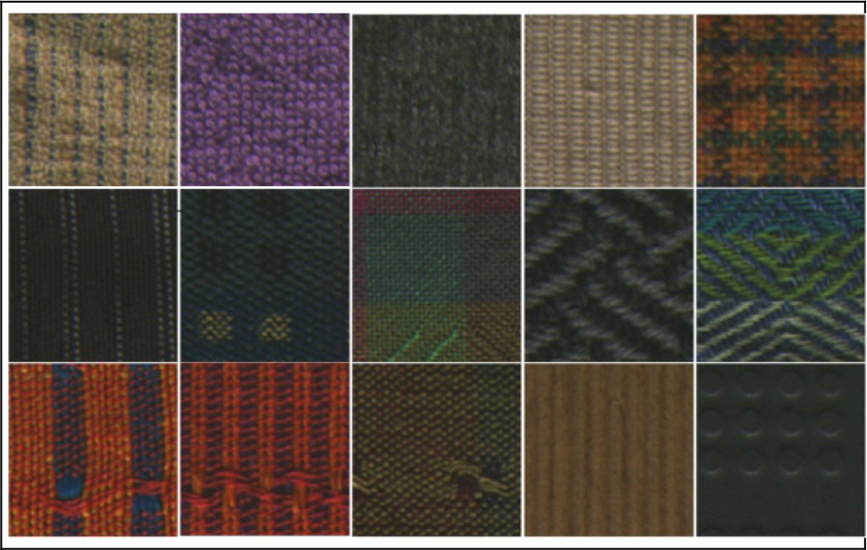
From the Vistex database, the 512×512 colour images dataset was chosen. The 31 image texture pairs were chosen from this database, where the first image was excluded for training and the second for testing. The texture window with dimensions of 64×64 pixels was used (16 textures for training and 16 for testing). An example of Vistex database is shown in Fig. 4.

Figure 4.

Example of Vistex database of training and testing texture pairs: a), b) c) are training images; d), e) and f) are testing images

For all experiments on GLCM, the parameters' distance d=1 and angles $θ = 0 °, 45 °, 90 °, 135 °$ were used. As mentioned above, only one feature, “homogeneity”, was used. The scale invariant texture pattern is provided by standardization of the total pairs of pixels, as defined in (2).

For GF, 30 banks in six orientations and five scales based on standard MPEG-7 (homogeneous texture descriptor [23,24]) were used.

Two simple software scripts for annotation and classification were created. The first script was used for the creation of an annotated database, where the training databases are at the input and the extracted feature vectors, exported into an XML file, are at the output. The second script was created for texture classification, through which the images from the testing databases are classified into appropriate classes by SVM and the results are evaluated by P, R and F1 score.

5.2. Experimental results

The texture classification results achieved on the Outex TC_00013 and Vistex databases are shown in Fig. 5. The best results for grey-level texture description were obtained by GF, and showed F1 reaching almost 80%. The GLCM with one feature (homogeneity) reached about 50%. After applying these methods to separate colour channels, a huge increase of retrieval precision for GLCM was obtained. More specifically, GLCM reached almost 80% of F1 for both databases. The retrieval precision of GF for separate colour channels increases by only a few percent. The highest precision for colour texture retrieval was obtained by the modification of GLCM called CLCM, where F1 reached over 90%. The detailed results of all experiments are shown in Tab. 1.

Figure 5.

Comparison of results for Outex TC_00013 dataset

Table 2.

The experimental results of P, R and F1 for databases Outex TC_00013 and Vistex

	Outex TC_00013			Vistex
	P	R	F1	P	R	F1
GLCM-grey	51,25	50,44	49,48	46,58	45,98	43,48
GFB-grey	80,39	80,15	79,43	76,68	72,32	70,69
CGLCM-rgb	81,84	80,44	79,76	73,39	71,88	69,62
CGLCM-hsv	80,78	80,29	79,72	81,05	79,02	78,35
CGFB-rgb	89,3	89,41	89,04	78,71	76,79	73,16
CGFB-hsv	84,17	83,38	83,01	84,92	81,25	80,33
CLCM-rgb	93,27	92,65	92,42	85,25	84,82	83,94
CLCM-hsv	90,95	90,74	90,56	92,57	91,52	90,97

The table shows the P, R and F1 score for all descriptors and both databases. Graphical representations of obtained results are presented in Figs. 5 and 6.

Figure 6.

Comparison of results for Vistex dataset

6. Conclusion

In this paper, research on extraction and classification of colour texture information was presented. Initially, GLCM and GF methods for the extraction of grey-level texture features and their use on separate channels in the colour image were experimentally tested. These results led us to apply the GLCM method on colour vector data and thus we produced the CLCM method. The experiments were carried out on the Vistex and Outex databases by using the RBF-based SVM classification. The experimental results confirm that the proposed CLCM method achieved an F1 score approximately 40% higher than the basic GLCM method, demonstrating over 90% success in colour texture classification.

In the future, the application of various combinations of GLCM features on the CLCM principle and also classification for specific applications will be researched.

Footnotes

7. Acknowledgments

This contribution is the result of the project's implementation at the Centre of Excellence for Systems and Services of Intelligent Transport, ITMS 26220120050. It was supported by the Research & Development Operational Programme funded by the ERDF and by Project No. 1/0705/13, “Image elements' classification for semantic image description”, with the support of the Ministry of Education, Science, Research and Sport of the Slovak Republic..

References

Shapiro

L G

Atmosukarto

Cho

Lin

H J

Ruiz-Correa

Yuen

(2007) Similarity-based retrieval for biomedical applications, Case-Based Reasoning on Signals and Images, Ed. Perner

, Springer.

Elizabeth

D S

Nehemiah

H K

Retmin

Raj C S

Kannan

(2012) Computer-aided diagnosis of lung cancer based on analysis of the significant slice of chest computed tomography image, Image Processing, IET, vol. 6, no. 6, pp. 697–705.

Singh

Rao

D V

(2013) Recognition and identification of target images using feature based retrieval in UAV missions, Computer Vision, Pattern Recognition, Image Processing and Graphics (NCVPRIPG), 2013 Fourth National Conference, pp. 1–4, 18–21.

Zheng

Wen

Zhang

Jin

Xie

(2011) Compounded Face Image Retrieval Based on Vertical Web Image Retrieval, Chinagrid Conference (ChinaGrid), pp. 130–135, 22–23.

Xinjuan

Junfang

Qianming

(2011) Apparel image matting and applications in e-commerce, Information Technology and Artificial Intelligence Conference (ITAIC), 6th IEEE Joint International Conference, vol. 2, pp. 278–282, 20–22.

Thakare

V S

Patil

N N

(2014) Classification of texture using gray level co-occurrence matrix and self-organizing map, Electronic Systems, Signal Processing and Computing Technologies (ICESC), International Conference, pp. 350–355, 9–11.

Fan-Hui

(2009) Image retrieval using both color and texture features, Machine Learning and Cybernetics, International Conference, vol. 4, pp. 2228–2232, 12–15.

Rashedi

Nezamabadi-Pour

(2012) Improving the precision of CBIR systems by feature selection using binary gravitational search algorithm, Artificial Intelligence and Signal Processing (AISP), 16th CSI International Symposium, pp. 39–42, 2–3.

Wang

Zhang

Zhao

Z-Y

Zhang

Z-D

Zhang

H-X

(2008) A semantic description for content-based image retrieval, Machine Learning and Cybernetics, International Conference, vol. 5, pp. 2466–2469, 12–15.

10.

Huang

Zhi-Chun

Chan

P P K

W W Y

Yeung

D S

(2010) Content-based image retrieval using color moment and Gabor texture feature, Machine Learning and Cybernetics (ICMLC), International Conference, vol. 2, pp. 719–724, 11–14.

11.

Askoy

Haralic

R M

(2000) Using texture in image similarity and retrieval, Texture Analysis in Machine Vision, M. Pietikainen, Ed., vol. 20, pp. 129–149. World Scientific, Singapore.

12.

Paschos

(2001) Perceptually uniform color spaces for color texture analysis: an empirical evaluation, Image Processing, IEEE Transactions, vol. 10, no. 6, pp. 932–937.

13.

Mei

Androutsos

(2008) Color texture retrieval using wavelet decomposition on the hue/saturation plane, Multimedia and Expo, IEEE International Conference, pp. 877–880.

14.

Assefaa

Mansinhab

Tiampob

K F

Rasmussenc

Abdellad

(2012) Local quaternion Fourier transform and color image texture analysis, Signal Processing, vol. 90, issue 6, pp. 1825–1835, ISSN 0165-1684.

15.

Mutasem

K S A

Khairuddin

B O

Shahrul

A N

Almarashdah

(2010) Fish recognition based on robust features extraction from color texture measurements using back-propagation classifier, Journal of Theoretical and Applied Information Technology, vol. 18, no. 1, Paper ID: 1401 -JATIT-2K10.

16.

Choi

J-Y

Y-M

Plataniotis

K N

(2012) Color local texture features for color face recognition, IEEE Transactions on Image Processing, vol. 21, no. 3, pp. 1366–1380.

17.

Hossain

Parekh

(2010) Extending GLCM to include color information for texture recognition, International Conference on Modeling, Optimization and Computing, Book Series: AIP Conference Proceedings, vol. 1298, pp. 583–588, ISSN: 0094-243X, ISBN: 978-0-7354-0854-8.

18.

Benco

Hudec

(2007) Novel Method for Color Texture Features Extraction Based on GLCM”, Radioengineering, Vol.16, No.4, pp. 64–67, ISSN 1210-2512.

19.

Haralick

R M

Shanmugam

Its'Hak

Dinstein

(1973) Textural features for image classification, Systems, Man and Cybernetics, IEEE Transactions, vol. SMC-3, no. 6, pp. 610–621.

20.

Haralick

R M

(1979) Statistical and structural approaches to texture, Proc. of the IEEE, 67, pp. 786–804.

21.

Nikoo

Talebi

Mirzaei

(2011) A supervised method for determining displacement of gray level co-occurrence matrix, Machine Vision and Image Processing (MVIP), 7th Iranian, pp. 1–5, 16–17.

22.

Manjunath

B S

W Y

(1996) Texture features for browsing and retrieval of image data, Pattern Analysis and Machine Intelligence, IEEE Transactions, vol. 18, no. 8, pp. 837–842.

23.

Y M

Kim

Kang

H K

Manjunath

B S

Kim

(2001) MPEG-7 Homogeneous texture descriptor ETRI Journal, vol. 23, no. 2, ISSN 2233-7326.

24.

Manjunath

B S

Salembier

Sikora

(2003) Introduction to MPEG-7 Multimedia Content Description Interface, ISBN: 0-471-48678-7.

25.

Muniz

Corrales

J A

(2006) Novel techniques for color texture classification, IPCV'06 Proceedings, pp. 114–120.

26.

Paschos

(2001) Perceptually uniform color spaces for color texture analysis: an empirical evaluation, Image Processing, IEEE Transactions, vol. 10, No. 6, pp. 932–937.

27.

Chang

Lin

C J

(2013) LIBSVM: a Library for Support Vector Machines (datasheet), Available: http://www.csie.ntu.edu.tw/~cjlin/papers/libsvm.pdf, Accessed on 25 Nov 2013.

28.

Cortes

Vapnik

(1995) Support vector networks. Machine Learning, vol. 20, issue 3, pp. 273–297.

29.

Haykin

(1998) Neural Network: A Comprehensive Foundation, Prentice Hall PTR Upper Saddle River, New Jersey, ISBN: 0132733501.

30.

Gao

Zhang

Guo

(2011) Multiple features-based image retrieval, Broadband Network and Multimedia Technology (IC-BNMT), 4th IEEE International Conference, pp. 240–244, 28–30.

31.

Lukac

Hudec

Benco

Kamencay

Dubcova

Zachariasova

(2011) Simple comparison of image segmentation algorithms based on evaluation criterion, Radioelektronika, 21st International Conference, pp. 1–4, 19–20.

32.

Ojala

(2002) Outex—new framework for empirical evaluation of texture analysis algorithms, Proceedings of the 16th International Conference on Pattern Recognition, vol. 1, QuWebec, Canada, pp. 701–706.

33.

MITMediaLab (1995) Vision texture, VisTexdatabase, Available: http://wwwhite.media.mit.edu/vismod/imagery/VisionTexture/vistex.html, Accessed on 14 Oct 2013.