Optimal Design of Water Treatment Facilities Under Nonlinear Conditions with Uncertainty Based on Flexible Tolerance Concept

Flexible tolerance concept

There are two types of difficulty for solving NLP problems. First, in the process of calculation, the constraints are difficult to satisfy for reaching the optimal solution. Next, even if the optimal solution is obtained, many pull-in operations are required to suffice the constraints at all times. Therefore, the concept of flexible tolerance is proposed in this research by allowing a tolerance for each constraint. In the process of calculation, the tolerance is reached gradually; it then approaches zero when the optimal solution is reached. The problem is assumed as follows: \documentclass{aastex}\usepackage{amsbsy}\usepackage{amsfonts}\usepackage{amssymb}\usepackage{bm}\usepackage{mathrsfs}\usepackage{pifont}\usepackage{stmaryrd}\usepackage{textcomp}\usepackage{portland,xspace}\usepackage{amsmath,amsxtra}\pagestyle{empty}\DeclareMathSizes{10}{9}{7}{6}\begin{document}\begin{align*} min.- x_1 - x_2 \\ s.t. - x_1^2 - x_2^2 + 4 = 0 , \\ x_1 \geq 0 \\ x_2 \geq 0 \tag{1} \end{align*}\end{document}

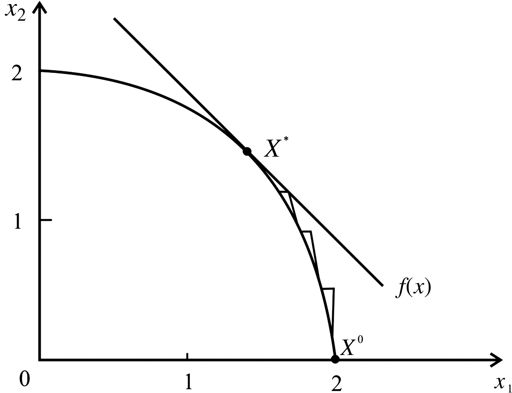
As shown in Fig. 1, the feasible region is an arc. If the initial point is X⁰ = (2 0), then it needs to move through the arc \documentclass{aastex}\usepackage{amsbsy}\usepackage{amsfonts}\usepackage{amssymb}\usepackage{bm}\usepackage{mathrsfs}\usepackage{pifont}\usepackage{stmaryrd}\usepackage{textcomp}\usepackage{portland,xspace}\usepackage{amsmath,amsxtra}\pagestyle{empty}\DeclareMathSizes{10}{9}{7}{6}\begin{document}$$- x_1^2 - x_2^2 - x_2^2 + 4 = 0$$\end{document} . Finally, this point converges at the optimal point \documentclass{aastex}\usepackage{amsbsy}\usepackage{amsfonts}\usepackage{amssymb}\usepackage{bm}\usepackage{mathrsfs}\usepackage{pifont}\usepackage{stmaryrd}\usepackage{textcomp}\usepackage{portland,xspace}\usepackage{amsmath,amsxtra}\pagestyle{empty}\DeclareMathSizes{10}{9}{7}{6}\begin{document}$$X^* = (2 / {\sqrt 2} \ \ 2 / {\sqrt 2})$$\end{document} . It moves along the line direction and walks a very short way at first and must pull in the feasible region. In the next step, it forwards the straight line direction and repeats the same pull-in operations. However, this process wastes much computation time, because the convergent rate is too slow. Hence, a new concept of tolerance drawn on Paviani's and Himmeblau's (1972) research is proposed (Paviani and Himmelban, 1969).

OPEN IN VIEWER

FIG. 1.

Model solution when constraint is curve.

In the beginning of the solving procedure, a tolerance is introduced to every constraint. Within the tolerance range, the constraint is assumed to be satisfied. There are three cases to be considered:

The points that satisfy are as follows:

(1) h(x) = 0, then it is feasible.

Where h(x) is the constraint.

In each step, the tolerance is gradually reduced so that it can finally approach zero when the optimal solution is reached.

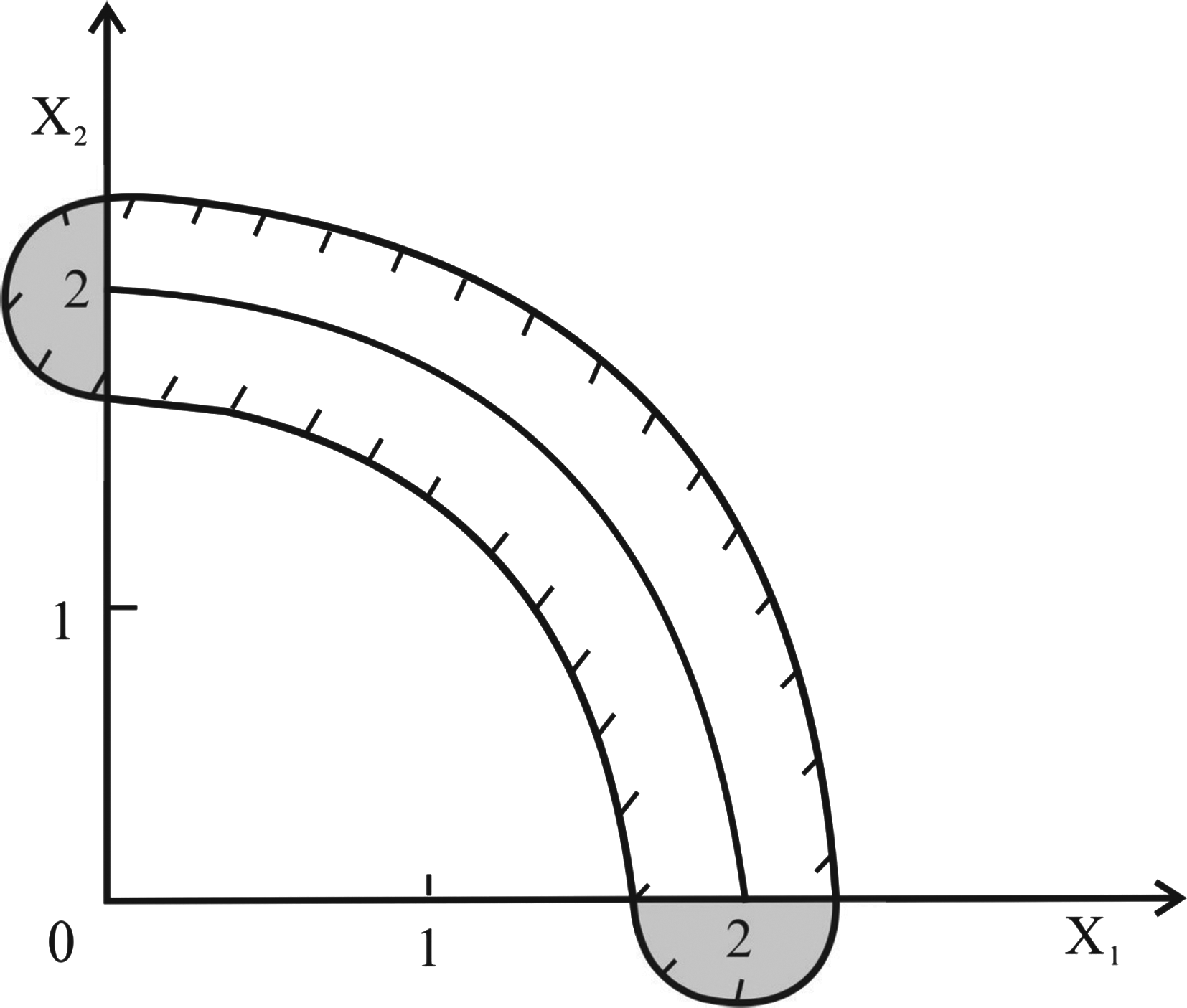
Figure 2 shows the geometry description of the concept of tolerance. When the problem has more than one constraint, as shown by Equation (2), all constraints can be combined for discussing their overall tolerance, which is presented as follows: \documentclass{aastex}\usepackage{amsbsy}\usepackage{amsfonts}\usepackage{amssymb}\usepackage{bm}\usepackage{mathrsfs}\usepackage{pifont}\usepackage{stmaryrd}\usepackage{textcomp}\usepackage{portland,xspace}\usepackage{amsmath,amsxtra}\pagestyle{empty}\DeclareMathSizes{10}{9}{7}{6}\begin{document}\begin{align*} {\rm min.} f(x) \\ s.t. \ g_i (x) \ge 0, \ i = 1, 2, \ldots.I \\ h_j(x) = 0, \ j = 1,2, \ldots.J \tag{2} \end{align*}\end{document}

OPEN IN VIEWER

FIG. 2.

Geometry description of the tolerance concept.

Suppose that U_i is a Heaviside operator, \documentclass{aastex}\usepackage{amsbsy}\usepackage{amsfonts}\usepackage{amssymb}\usepackage{bm}\usepackage{mathrsfs}\usepackage{pifont}\usepackage{stmaryrd}\usepackage{textcomp}\usepackage{portland,xspace}\usepackage{amsmath,amsxtra}\pagestyle{empty}\DeclareMathSizes{10}{9}{7}{6}\begin{document}\begin{align*} U_{i} = \begin{cases}0 , \quad if \quad g_i (x) \geq 0 \\ 1 , \quad if \quad g_i (x) < 0\end{cases} \tag{3} \end{align*}\end{document}

T(x), which is always positive, is defined as the following: \documentclass{aastex}\usepackage{amsbsy}\usepackage{amsfonts}\usepackage{amssymb}\usepackage{bm}\usepackage{mathrsfs}\usepackage{pifont}\usepackage{stmaryrd}\usepackage{textcomp}\usepackage{portland,xspace}\usepackage{amsmath,amsxtra}\pagestyle{empty}\DeclareMathSizes{10}{9}{7}{6}\begin{document}\begin{align*} {\rm T} ({\rm X}) = \sum_{i = 1}^I U_i g_i^2 (x) + \sum_{j = 1}^J h_j^2 (x) \tag{4} \end{align*}\end{document}

to mean that all constraints should be satisfied. When T(X) = 0, all constraints are satisfied, and X is a feasible solution. When \documentclass{aastex}\usepackage{amsbsy}\usepackage{amsfonts}\usepackage{amssymb}\usepackage{bm}\usepackage{mathrsfs}\usepackage{pifont}\usepackage{stmaryrd}\usepackage{textcomp}\usepackage{portland,xspace}\usepackage{amsmath,amsxtra}\pagestyle{empty}\DeclareMathSizes{10}{9}{7}{6}\begin{document}$$0 \leq {\rm T} ({\rm X}) \ {\leq} \in$$\end{document} , X is a near feasible; when \documentclass{aastex}\usepackage{amsbsy}\usepackage{amsfonts}\usepackage{amssymb}\usepackage{bm}\usepackage{mathrsfs}\usepackage{pifont}\usepackage{stmaryrd}\usepackage{textcomp}\usepackage{portland,xspace}\usepackage{amsmath,amsxtra}\pagestyle{empty}\DeclareMathSizes{10}{9}{7}{6}\begin{document}$${\rm T} ({\rm X}) > \in$$\end{document} , X is an infeasible so that it should move toward the feasible region.

When the problem is presented in the form of equation (1) with \documentclass{aastex}\usepackage{amsbsy}\usepackage{amsfonts}\usepackage{amssymb}\usepackage{bm}\usepackage{mathrsfs}\usepackage{pifont}\usepackage{stmaryrd}\usepackage{textcomp}\usepackage{portland,xspace}\usepackage{amsmath,amsxtra}\pagestyle{empty}\DeclareMathSizes{10}{9}{7}{6}\begin{document}$$\in = 1 / 3$$\end{document} , Fig. 3 represents near feasible region. The two semicircles are the tolerance for x₁ ≥ 0 and x₂ ≥ 0, respectively.

OPEN IN VIEWER

FIG. 3.

The quasi-feasible region obtained by combining all constraints.

Hestenes' method of multipliers

One of the methods to solve the NLP is the use of a combined technique. The objective function and constraints are combined by using some special algorithm to become an unconstrained NLP. The solution remains the same as for the original problem, whereas the unconstrained NLP makes it much easier than constrained NLP for obtaining the solution. Hence, this method of functional conversion is favored by most researchers who have continually proposed new methods to convert functions. Among the numerous conversion functions such as interior penalty value, exterior penalty value, and method of multipliers, the multipliers method is considered the best (Hwang, 1993; Martinez, 2003).

For the NLP problem, as Eq. (2):

The objective function and constraints are combined into Eq. (5): \documentclass{aastex}\usepackage{amsbsy}\usepackage{amsfonts}\usepackage{amssymb}\usepackage{bm}\usepackage{mathrsfs}\usepackage{pifont}\usepackage{stmaryrd}\usepackage{textcomp}\usepackage{portland,xspace}\usepackage{amsmath,amsxtra}\pagestyle{empty}\DeclareMathSizes{10}{9}{7}{6}\begin{document}\begin{align*} min.\ p (x) {=}f (x) {+}R \left[\sum_{i = 1}^I U_i g_i^2 (x) + \sum_{j = 1}^J h_j^2 (x) \right] \tag{5} \end{align*}\end{document}

where

U_i: Heaviside operator \documentclass{aastex}\usepackage{amsbsy}\usepackage{amsfonts}\usepackage{amssymb}\usepackage{bm}\usepackage{mathrsfs}\usepackage{pifont}\usepackage{stmaryrd}\usepackage{textcomp}\usepackage{portland,xspace}\usepackage{amsmath,amsxtra}\pagestyle{empty}\DeclareMathSizes{10}{9}{7}{6}\begin{document}\begin{align*} U_i = \begin{cases}0 , \quad if \quad g_i (x) \geq 0 \\ 1 , \quad if \quad g_i (x) < 0\end{cases} \tag{6} \end{align*}\end{document}

R: penalty value

When R approaches ∞, then the optimal solution X* for Equation (5) is the X* for Equation (2).

Flexible tolerance

Regarding the flexible concept of tolerance, the tolerance is defined as follows: \documentclass{aastex}\usepackage{amsbsy}\usepackage{amsfonts}\usepackage{amssymb}\usepackage{bm}\usepackage{mathrsfs}\usepackage{pifont}\usepackage{stmaryrd}\usepackage{textcomp}\usepackage{portland,xspace}\usepackage{amsmath,amsxtra}\pagestyle{empty}\DeclareMathSizes{10}{9}{7}{6}\begin{document}\begin{align*} {\rm T} ({\rm X}) = \sum_{i = 1}^I U_i g_i^2 (x) + \sum_{j = 1}^J h_j^2 (x) \tag{7} \end{align*}\end{document}

The minimum value of F(X, λ, μ, R) is calculated for each stage.

Assuming \documentclass{aastex}\usepackage{amsbsy}\usepackage{amsfonts}\usepackage{amssymb}\usepackage{bm}\usepackage{mathrsfs}\usepackage{pifont}\usepackage{stmaryrd}\usepackage{textcomp}\usepackage{portland,xspace}\usepackage{amsmath,amsxtra}\pagestyle{empty}\DeclareMathSizes{10}{9}{7}{6}\begin{document}\begin{align*} F (X , \lambda , \mu , R) = f (x) + \sum_{j = 1}^J \lambda_j h_j (x) + R \sum_{j = 1}^J h_j{^2} (x) \\ \qquad\quad - \sum_{i = 1}^I \mu_i {\overline {g_i}} (x) + R \sum_{i = 1}^I {\overline{g_i}{^2}} (x) \tag{8} \end{align*}\end{document}

where

λ; μ: Lagrange multiplier

R: penalty value, a constant during the process of solving the problem. \documentclass{aastex}\usepackage{amsbsy}\usepackage{amsfonts}\usepackage{amssymb}\usepackage{bm}\usepackage{mathrsfs}\usepackage{pifont}\usepackage{stmaryrd}\usepackage{textcomp}\usepackage{portland,xspace}\usepackage{amsmath,amsxtra}\pagestyle{empty}\DeclareMathSizes{10}{9}{7}{6}\begin{document}\begin{align*} \begin{cases} \lambda_{n + 1 , j} = \lambda_{n , j} + 2 Rh_i (x) \\ \mu_{n + 1 , j} = \mu_{n , 1} - 2 R {\overline {g_j}} (x) \end{cases} \tag{9} \end{align*}\end{document}

The difference between two functions (F) in two consecutive stages should be equal to or greater than zero, or \documentclass{aastex}\usepackage{amsbsy}\usepackage{amsfonts}\usepackage{amssymb}\usepackage{bm}\usepackage{mathrsfs}\usepackage{pifont}\usepackage{stmaryrd}\usepackage{textcomp}\usepackage{portland,xspace}\usepackage{amsmath,amsxtra}\pagestyle{empty}\DeclareMathSizes{10}{9}{7}{6}\begin{document}\begin{align*} F (X , \lambda_{n + 1} , \mu_{n + 1} , R) - F (X , \lambda_n , \mu_n , R) \geq 0 \tag{10} \end{align*}\end{document}

This is the basis of the convergence for the multipliers method. Based on the research conducted by (Reklaitis et al., 1983), Equation (2) can be transformed as follows: \documentclass{aastex}\usepackage{amsbsy}\usepackage{amsfonts}\usepackage{amssymb}\usepackage{bm}\usepackage{mathrsfs}\usepackage{pifont}\usepackage{stmaryrd}\usepackage{textcomp}\usepackage{portland,xspace}\usepackage{amsmath,amsxtra}\pagestyle{empty}\DeclareMathSizes{10}{9}{7}{6}\begin{document}\begin{align*} F (X , \sigma , \tau , R) = f (x) + R \sum_{i = 1}^I \left[< g_i (x) + \sigma_i >^2 - \sigma_i{^2} \right] \\ \quad \quad\ \ + R \sum_{j = 1}^J \left[(h_j (x) + \tau_j)^2 \ {-} \tau_j{^2} \right] \tag{11} \end{align*}\end{document}

where

< >: means that if the value inside the < > is greater than zero, then < > = 0; if it is smaller than zero (e.g., a), then < > = a (a < 0).

and \documentclass{aastex}\usepackage{amsbsy}\usepackage{amsfonts}\usepackage{amssymb}\usepackage{bm}\usepackage{mathrsfs}\usepackage{pifont}\usepackage{stmaryrd}\usepackage{textcomp}\usepackage{portland,xspace}\usepackage{amsmath,amsxtra}\pagestyle{empty}\DeclareMathSizes{10}{9}{7}{6}\begin{document}\begin{align*} \begin{cases} \sigma_{n + 1 , i} = < g_i (x) + \sigma_{n , i} > ;\ \qquad i = 1 , 2 , \ldots , I \\ \tau_{n + 1 , j} = h_j (x) + \tau_{n , j} ; \ \ \qquad \quad j = 1 , 2 , \ldots , J\end{cases} \tag{12} \end{align*}\end{document}

The minimum value for Equation (11) can be found in every step. Meanwhile, the values of σ & τ can be modified based on Equation (12).

When σ_n+1 = σ _n , τ_n+1 = τ _n , then the convergence is in the optimal solution.

If ∇F(Xⁿ, σ _n , τ _n , R) = 0, and σ_n+1 = σ _n , τ_n+1, = τ _n , then Xⁿ is the Kuhn-Tucker stationary point for Equation (2).

The Hessian matrix included in Equation (11) is expressed as follows: \documentclass{aastex}\usepackage{amsbsy}\usepackage{amsfonts}\usepackage{amssymb}\usepackage{bm}\usepackage{mathrsfs}\usepackage{pifont}\usepackage{stmaryrd}\usepackage{textcomp}\usepackage{portland,xspace}\usepackage{amsmath,amsxtra}\pagestyle{empty}\DeclareMathSizes{10}{9}{7}{6}\begin{document}\begin{align*} \nabla^2 F (X) = \nabla^2 f (x) + 2R \sum [< g_i (x) + \sigma_i > \nabla^2 g_i (x) + \nabla^2 g_i^2 (x)] \\ + 2R \sum [(h_j (x) + \tau_j) \nabla^2 h_j (x) + \nabla h_j^2 (x)] \tag{13} \end{align*}\end{document}

If g_i (x) & h_j(x) are linear constraints, then Equation (13) can be simplified to \documentclass{aastex}\usepackage{amsbsy}\usepackage{amsfonts}\usepackage{amssymb}\usepackage{bm}\usepackage{mathrsfs}\usepackage{pifont}\usepackage{stmaryrd}\usepackage{textcomp}\usepackage{portland,xspace}\usepackage{amsmath,amsxtra}\pagestyle{empty}\DeclareMathSizes{10}{9}{7}{6}\begin{document}\begin{align*} \nabla^2 F (X) = \nabla^2 f (x) + 2R \sum_{i = 1}^I \nabla g_i^2 (x) + 2R \sum_{j = 1}^J \nabla h_j^2 (x) \tag{14} \end{align*}\end{document}

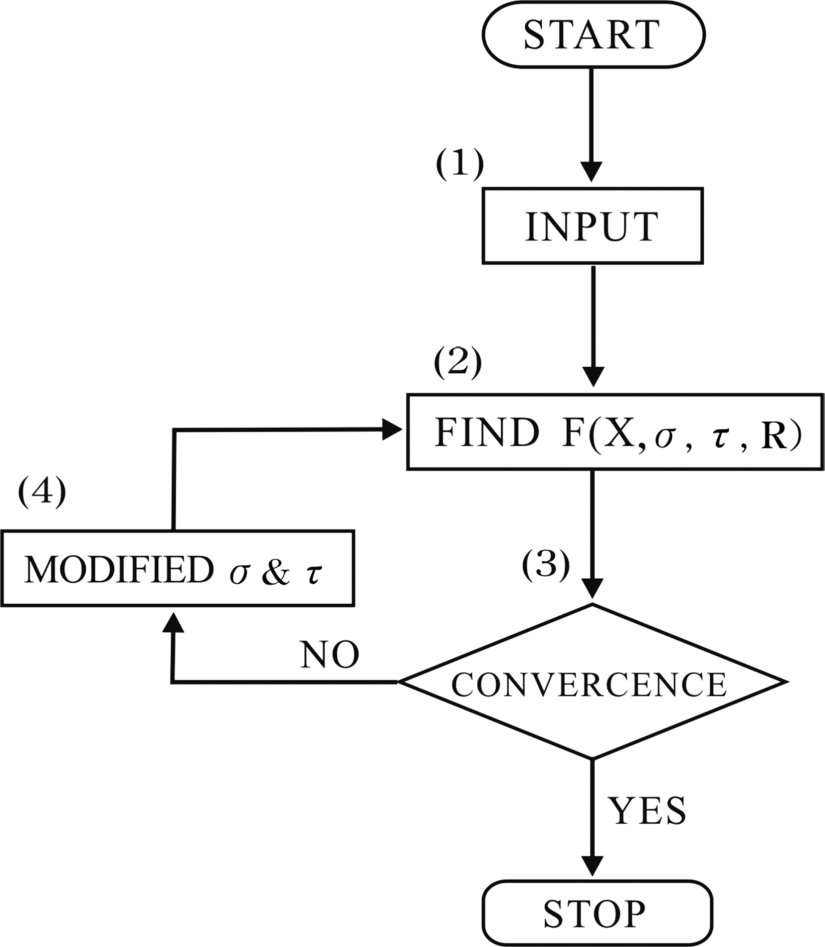
∇² F(X) is independent of either σ or τ. So, the convergence will not be influenced by the shape of function F (Madani et al., 2007). In Fig. 4 below, a flow chart of the multipliers method with tolerance concept is shown:

OPEN IN VIEWER

FIG. 4.

Flowchart of the multiplier method with tolerance concept.

The objective function

The actual objective function for the selected existing plant is as follows: \documentclass{aastex}\usepackage{amsbsy}\usepackage{amsfonts}\usepackage{amssymb}\usepackage{bm}\usepackage{mathrsfs}\usepackage{pifont}\usepackage{stmaryrd}\usepackage{textcomp}\usepackage{portland,xspace}\usepackage{amsmath,amsxtra}\pagestyle{empty}\DeclareMathSizes{10}{9}{7}{6}\begin{document}\begin{align*} {\rm min}. \ \ Z = \ & 0.572 \ X_1 - 0.00289 \ X_1^2 + 0.0422 \ X_2 - 0.0000449 \ X{_2^2} \\\quad & + 0.00386 \ X_3 + 0.000136 \ X{_3^2} + 0.00775 \ X_4 \\ \quad & - 0.00000052 \ X_2^4 + 0.001449 \ X_5 - 0.000000063 \ X{_5^2} \\ \quad & + 0.0148 \ X_6 - 0.000025 \ X{_6^2} \\ \quad & + 0.844 \ X_7 - 0.00406 \ X{_7^2} \tag{15} \end{align*}\end{document}

The derivation of structural constraints are considered as parameters representing input water quality, output water quality, treatment efficiency, detention time, operating limit, and treatment characteristics.

Stochastic constraints

Stochastic constraints transformation

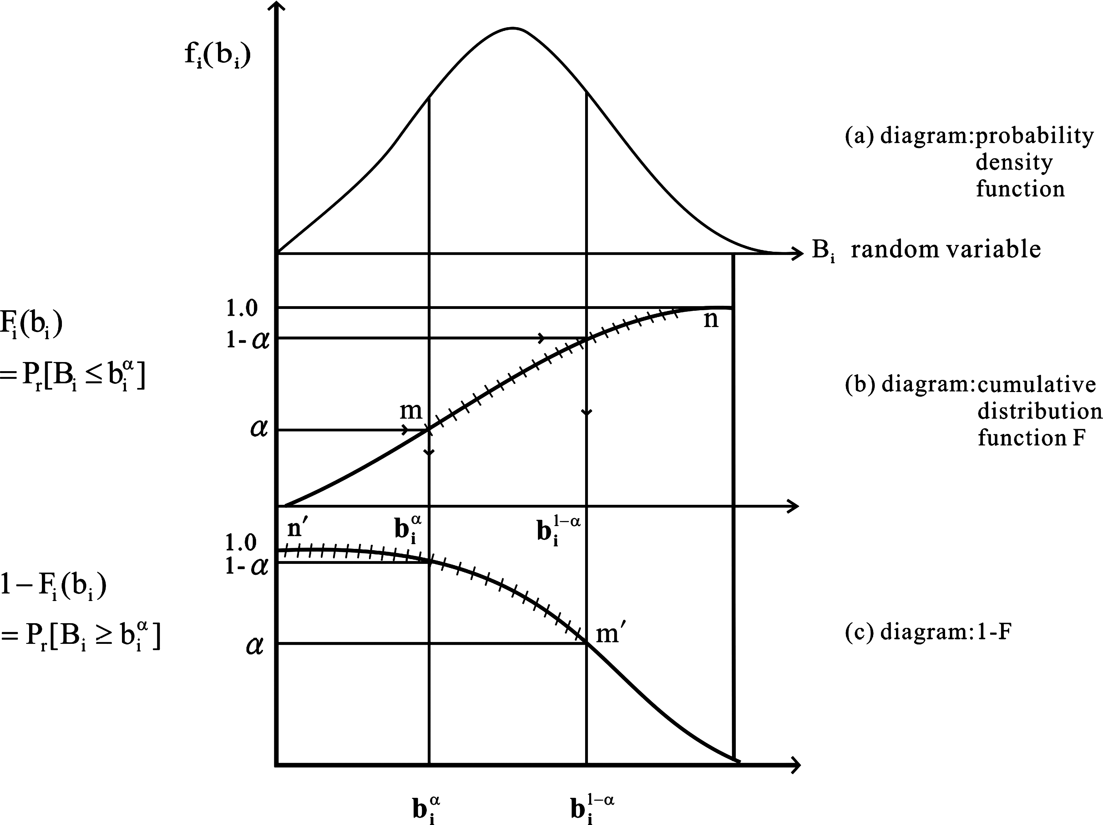
Equations (16) to (23) reveal that the stochastic characteristic has been included in each constraint so that the inverse of the marginal cumulative distribution function of input water quality parameters needs to be solved. Under such circumstances, the stochastic constraints can be transferred to certainty forms. The relationship between probability and \documentclass{aastex}\usepackage{amsbsy}\usepackage{amsfonts}\usepackage{amssymb}\usepackage{bm}\usepackage{mathrsfs}\usepackage{pifont}\usepackage{stmaryrd}\usepackage{textcomp}\usepackage{portland,xspace}\usepackage{amsmath,amsxtra}\pagestyle{empty}\DeclareMathSizes{10}{9}{7}{6}\begin{document}$${\rm b}_{\rm i}^{\alpha}$$\end{document} is shown in Fig. 6. If \documentclass{aastex}\usepackage{amsbsy}\usepackage{amsfonts}\usepackage{amssymb}\usepackage{bm}\usepackage{mathrsfs}\usepackage{pifont}\usepackage{stmaryrd}\usepackage{textcomp}\usepackage{portland,xspace}\usepackage{amsmath,amsxtra}\pagestyle{empty}\DeclareMathSizes{10}{9}{7}{6}\begin{document}$${\rm Pr} [g_{i (x)} \leq B_i] \geq \alpha , \ and \ \alpha = 0.15 , b_i^{\alpha} = 100 , b_i^{1 - \alpha} = 180$$\end{document} diagram (b) can be used to convert the constrain, which contains probability the constraint, into deterministic equivalent. Since pr[.] is greater than 0.15, the answer is in the curve interval (mn), and the corresponding \documentclass{aastex}\usepackage{amsbsy}\usepackage{amsfonts}\usepackage{amssymb}\usepackage{bm}\usepackage{mathrsfs}\usepackage{pifont}\usepackage{stmaryrd}\usepackage{textcomp}\usepackage{portland,xspace}\usepackage{amsmath,amsxtra}\pagestyle{empty}\DeclareMathSizes{10}{9}{7}{6}\begin{document}$${\rm b}_{\rm i}^{\alpha}$$\end{document} is equal to 100; the solution is g_i(x) ≥ 100, which is inconsistent with the original problem statement that g_i (x) ≤ B_i. Hence, diagram (c) is used to justify the conversion procedure. Since pr[.] ≥ 0.15, the answer is on the curve (m′n′); the corresponding \documentclass{aastex}\usepackage{amsbsy}\usepackage{amsfonts}\usepackage{amssymb}\usepackage{bm}\usepackage{mathrsfs}\usepackage{pifont}\usepackage{stmaryrd}\usepackage{textcomp}\usepackage{portland,xspace}\usepackage{amsmath,amsxtra}\pagestyle{empty}\DeclareMathSizes{10}{9}{7}{6}\begin{document}$${\rm b}_{\rm i}^{1 - \alpha}$$\end{document} equals to 180; so that the solution is g_i (x) ≤ 180. This coincides with the original problem statement g_i (x) ≤ B_i.

OPEN IN VIEWER

FIG. 6.

Cumulative density function transformation concept.

Equation (20) is expressed as \documentclass{aastex}\usepackage{amsbsy}\usepackage{amsfonts}\usepackage{amssymb}\usepackage{bm}\usepackage{mathrsfs}\usepackage{pifont}\usepackage{stmaryrd}\usepackage{textcomp}\usepackage{portland,xspace}\usepackage{amsmath,amsxtra}\pagestyle{empty}\DeclareMathSizes{10}{9}{7}{6}\begin{document}\begin{align*} - \frac {19200} {Q} X_1 - \frac {9840} {Q} X_2 \geq 35 - F_ {A1}^ {- 1} (1 - \alpha) \end{align*}\end{document}

is the same as Eq. (24) \documentclass{aastex}\usepackage{amsbsy}\usepackage{amsfonts}\usepackage{amssymb}\usepackage{bm}\usepackage{mathrsfs}\usepackage{pifont}\usepackage{stmaryrd}\usepackage{textcomp}\usepackage{portland,xspace}\usepackage{amsmath,amsxtra}\pagestyle{empty}\DeclareMathSizes{10}{9}{7}{6}\begin{document}\begin{align*} pr [A_3 \leq 35 + \frac {19200} {Q} X_1 \frac {9480} {Q} X_2] \leq \alpha \tag{24} \end{align*}\end{document}

Using the above description of conversion algorithm, we will obtain

\documentclass{aastex}\usepackage{amsbsy}\usepackage{amsfonts}\usepackage{amssymb}\usepackage{bm}\usepackage{mathrsfs}\usepackage{pifont}\usepackage{stmaryrd}\usepackage{textcomp}\usepackage{portland,xspace}\usepackage{amsmath,amsxtra}\pagestyle{empty}\DeclareMathSizes{10}{9}{7}{6}\begin{document}$$K = {\rm b}_1^{1 - \alpha}$$\end{document} , where K is constant, and K > 0, and hence \documentclass{aastex}\usepackage{amsbsy}\usepackage{amsfonts}\usepackage{amssymb}\usepackage{bm}\usepackage{mathrsfs}\usepackage{pifont}\usepackage{stmaryrd}\usepackage{textcomp}\usepackage{portland,xspace}\usepackage{amsmath,amsxtra}\pagestyle{empty}\DeclareMathSizes{10}{9}{7}{6}\begin{document}\begin{align*} K = \left[\begin{matrix}b_i^{\alpha} & & \hbox{\rm using diagram} ({\rm b}) \\ & {\rm when} & \\ b_i^{1 - \alpha} & & \hbox{\rm using diagram} ({\rm c}) \end{matrix} \right. \end{align*}\end{document}

and 1−α = complementary probability of α. \documentclass{aastex}\usepackage{amsbsy}\usepackage{amsfonts}\usepackage{amssymb}\usepackage{bm}\usepackage{mathrsfs}\usepackage{pifont}\usepackage{stmaryrd}\usepackage{textcomp}\usepackage{portland,xspace}\usepackage{amsmath,amsxtra}\pagestyle{empty}\DeclareMathSizes{10}{9}{7}{6}\begin{document}\begin{align*} {\rm A}_3 = {\rm A}_1 - \frac {19200} {{\rm Q}} {\rm X}_1 - \frac {9480} {{\rm Q}} {\rm X}_2 \geq 35 \tag{25} \end{align*}\end{document} \documentclass{aastex}\usepackage{amsbsy}\usepackage{amsfonts}\usepackage{amssymb}\usepackage{bm}\usepackage{mathrsfs}\usepackage{pifont}\usepackage{stmaryrd}\usepackage{textcomp}\usepackage{portland,xspace}\usepackage{amsmath,amsxtra}\pagestyle{empty}\DeclareMathSizes{10}{9}{7}{6}\begin{document}\begin{align*} A_1 & = K \\ {\rm K} & \geq 35 + \frac {19200} {{\rm Q}} {\rm X}_1 + \frac {9480} {{\rm Q}} {\rm X}_2 \tag{26} \end{align*}\end{document}

Rearranging the terms in Eq. (26), one obtains: \documentclass{aastex}\usepackage{amsbsy}\usepackage{amsfonts}\usepackage{amssymb}\usepackage{bm}\usepackage{mathrsfs}\usepackage{pifont}\usepackage{stmaryrd}\usepackage{textcomp}\usepackage{portland,xspace}\usepackage{amsmath,amsxtra}\pagestyle{empty}\DeclareMathSizes{10}{9}{7}{6}\begin{document}\begin{align*} \frac {- 19200} {{\rm Q}} {\rm X}_1 + \frac {9480} {{\rm Q}} {\rm X}_2 \geq 35 - {\rm K} \tag{27} \end{align*}\end{document}

Deterministic equivalent for the stochastic model

Since the objective function excluded the probability item, it is not convertible.

Constraints are as follows:

The total alkalinity for coagulation is presented as follows: \documentclass{aastex}\usepackage{amsbsy}\usepackage{amsfonts}\usepackage{amssymb}\usepackage{bm}\usepackage{mathrsfs}\usepackage{pifont}\usepackage{stmaryrd}\usepackage{textcomp}\usepackage{portland,xspace}\usepackage{amsmath,amsxtra}\pagestyle{empty}\DeclareMathSizes{10}{9}{7}{6}\begin{document}\begin{align*} \frac {- 19200} {{\rm Q}} {\rm X}_1 - \frac {9480} {{\rm Q}} {\rm X}_2 \geq 35 - {\rm F}_ {{\rm A}_1^{- 1}} (\alpha) \tag{20} \end{align*}\end{document}

That is, \documentclass{aastex}\usepackage{amsbsy}\usepackage{amsfonts}\usepackage{amssymb}\usepackage{bm}\usepackage{mathrsfs}\usepackage{pifont}\usepackage{stmaryrd}\usepackage{textcomp}\usepackage{portland,xspace}\usepackage{amsmath,amsxtra}\pagestyle{empty}\DeclareMathSizes{10}{9}{7}{6}\begin{document}\begin{align*} {\rm F}_ {{\rm A} 1} \left(35 + \frac {19200} {{\rm Q}} {X}_1 + \frac {9480} {{\rm Q}} {X}_2 \right) \leq \alpha \tag{28} \end{align*}\end{document}

or \documentclass{aastex}\usepackage{amsbsy}\usepackage{amsfonts}\usepackage{amssymb}\usepackage{bm}\usepackage{mathrsfs}\usepackage{pifont}\usepackage{stmaryrd}\usepackage{textcomp}\usepackage{portland,xspace}\usepackage{amsmath,amsxtra}\pagestyle{empty}\DeclareMathSizes{10}{9}{7}{6}\begin{document}\begin{align*} pr \left[A_1 \leq 35 + \frac {19200} {Q} {\rm X}_1 + \frac {9480} {Q} {\rm X}_2 \right] \leq \alpha \tag{29} \end{align*}\end{document}

Using diagram (b) in Fig. 6, if the decision maker, let α = 0.25 or 1 − α = 75%, and Q = 75000^CMD, then Eq. (30) can be easily obtained: \documentclass{aastex}\usepackage{amsbsy}\usepackage{amsfonts}\usepackage{amssymb}\usepackage{bm}\usepackage{mathrsfs}\usepackage{pifont}\usepackage{stmaryrd}\usepackage{textcomp}\usepackage{portland,xspace}\usepackage{amsmath,amsxtra}\pagestyle{empty}\DeclareMathSizes{10}{9}{7}{6}\begin{document}\begin{align*} 35 + \frac {19200} {75000} X_1 + \frac {9480} {75000} X_2 \leq 48.5 \tag{30} \end{align*}\end{document}

The corrosion control relationship is presented as follows when α < 0.6: \documentclass{aastex}\usepackage{amsbsy}\usepackage{amsfonts}\usepackage{amssymb}\usepackage{bm}\usepackage{mathrsfs}\usepackage{pifont}\usepackage{stmaryrd}\usepackage{textcomp}\usepackage{portland,xspace}\usepackage{amsmath,amsxtra}\pagestyle{empty}\DeclareMathSizes{10}{9}{7}{6}\begin{document}\begin{align*} 0.215 \ X_1 + 0.071 \ X_2 + 0.215 \ X_7 \leq - 0.54 \ (inconsistent) \tag{31} \end{align*}\end{document}

If α value is enlarged to 1.0 (α = 1.0), Eq. (32) can be obtained: \documentclass{aastex}\usepackage{amsbsy}\usepackage{amsfonts}\usepackage{amssymb}\usepackage{bm}\usepackage{mathrsfs}\usepackage{pifont}\usepackage{stmaryrd}\usepackage{textcomp}\usepackage{portland,xspace}\usepackage{amsmath,amsxtra}\pagestyle{empty}\DeclareMathSizes{10}{9}{7}{6}\begin{document}\begin{align*} \begin{split}0.215 \ X_1 + 0.071 \ X_2 + 0.215 \ X_7 \leq 4.14 \\\quad (\hbox{consistent but unreasonable})\end{split} \tag{32} \end{align*}\end{document}

The effluent water quality of the selected existing plant should be corrosive in some aspects. If this constraint is not neglected in the structural constraints, a feasible solution for this model is not available so that the sensitivity analysis is necessary to make the conclusion significant and meaningful.

The following equations are established using α = 0.25:

For the alum dosage for coagulation: \documentclass{aastex}\usepackage{amsbsy}\usepackage{amsfonts}\usepackage{amssymb}\usepackage{bm}\usepackage{mathrsfs}\usepackage{pifont}\usepackage{stmaryrd}\usepackage{textcomp}\usepackage{portland,xspace}\usepackage{amsmath,amsxtra}\pagestyle{empty}\DeclareMathSizes{10}{9}{7}{6}\begin{document}\begin{align*} X_2 > 109.4 \tag{33} \end{align*}\end{document}

For the effluent turbidity: \documentclass{aastex}\usepackage{amsbsy}\usepackage{amsfonts}\usepackage{amssymb}\usepackage{bm}\usepackage{mathrsfs}\usepackage{pifont}\usepackage{stmaryrd}\usepackage{textcomp}\usepackage{portland,xspace}\usepackage{amsmath,amsxtra}\pagestyle{empty}\DeclareMathSizes{10}{9}{7}{6}\begin{document}\begin{align*} 0.213 X_3 + X_4 + 0.126 X_5 + 7500 X_6 \geq 1847491 \tag{34} \end{align*}\end{document}

For the effluent coliform bacteria: \documentclass{aastex}\usepackage{amsbsy}\usepackage{amsfonts}\usepackage{amssymb}\usepackage{bm}\usepackage{mathrsfs}\usepackage{pifont}\usepackage{stmaryrd}\usepackage{textcomp}\usepackage{portland,xspace}\usepackage{amsmath,amsxtra}\pagestyle{empty}\DeclareMathSizes{10}{9}{7}{6}\begin{document}\begin{align*} - X_3 - 4.55 X_4 - 0.057 X_5 + 16200 X_6 \leq 13982985 \tag{35} \end{align*}\end{document}

Computer solutions

The software developed by (Kao et al., 2005) was tested and modified to assure that it is appropriate to be used in this research. The data input is done using two methods:

(1) Data such as N1(number of variables), NEQ (number of constraints containing “ = ”), NGE (number of constraints containing “<” or “>”), R(penalty value), and X^o (coordinates of the beginning and ending points) are input using the READ command.

(2) The objective function and constraints are input using the “SUB ROUTINE” function; the objective function is designated as SUBROUTINE FUN, whereas the constraints are designated as SUBROUTINE CON.

(3) Initial values are “0” for σ₀ and τ₀ so that \documentclass{aastex}\usepackage{amsbsy}\usepackage{amsfonts}\usepackage{amssymb}\usepackage{bm}\usepackage{mathrsfs}\usepackage{pifont}\usepackage{stmaryrd}\usepackage{textcomp}\usepackage{portland,xspace}\usepackage{amsmath,amsxtra}\pagestyle{empty}\DeclareMathSizes{10}{9}{7}{6}\begin{document}$$F (X , \sigma_0 , \tau_0 , R)$$\end{document} is made a standard penalty function.

(4) The value of penalty value R is input intuitively using values of 1, 10, 10², 10⁻¹, 10⁻², … , and so on. It is kept a constant during the problem solving process. In the actual scope of solution, the probability value α varies from 0.1 to 0.4 with intervals of 0.05.

Result analysis

Two methods based on the concept of tolerance, that is, the method of feasible directions and the multipliers method, have been developed in this research; they are solved using computer software. Due to the limited length of this article, only the multipliers method that leads to better results is presented in this article for demonstrating the theory and application of the flexible tolerance.

The quadratic regression cost function is used to obtain nonlinear objective function. The above computer program is applied to execute the calculation based on 10% of interest rate, 0.11017 of capital recovery factor, and 25 years of design life for the water treatment plant; the results show that when α value is less than 0.25 (α < 0.25), the mode has no solution; the optimal solution can be obtained only when α equals to 0.25. This finding indicates that the actual operation of the water treatment plant is subject to 25% risk or 75% reliability. Compared with the 50% reliability for water treatment plant designed using the traditional approach, the results obtained using the method proposed in this research is much better.

Table 1 lists the original design values and those obtained in this research. The solution of the proposed model is considered “exact solution.” The observation that the proposed model has significant solutions only when α value exceeds 0.25 is significant. It indicates that the lack of appropriate equipment for adding alkaline chemicals in the existing water treatment plant causes corrosive, treated effluent. In the flowchart shown in Fig. 5, if a new unit operation, that is, Unit #2′, is added between Unit #2 and Unit #3, a new variable, that is, X₂′, will be included in the model to indicate the lime dosage in kgs/h. As shown in Fig. 7, the modifications lead to optimal solution. As shown in Table 2, the modified model can be solved even if the α value equals to 0.01, thus indicating that the reliability is raised to 99.9%.

OPEN IN VIEWER

FIG. 7.

Adding unit#2′ to the original treatment flowchart.

The sensitivity analysis is usually conducted by varying the price coefficient (c_i), constants (b_i), and coefficient constant (a_ij) used in a model and changing the constraints and decision variables. Although not discussed in this article due to limited article length, the sensitivity analysis is more significant in effluent turbidity, corrosion control, and fecal coliform removal.