Viscosity Variations of Three-Component Mixtures Comprising an Alcohol,Various Common Groundwater Contaminants,and Water

Abstract

This study investigates the variations in fluid viscosity as water was continuously added to a mixture containing methanol and a common groundwater liquid contaminant. Three different liquid contaminants were considered, namely benzene, toluene, and trichloroethylene. Each methanol-contaminant mixture (50%–50% by volume) was initially a single-phase solution, but partitioned into a two-phase liquid–liquid system after the total water content of the system reached a critical value. After the mixture partitioned into a two-phase system, fluid viscosities of each liquid phase were determined as more water was added to the system. A modified falling-ball viscometer was used to determine the viscosity of each mixture. Results from the viscosity experiments showed that in the single-phase region, the observed mixture viscosity increased with increasing total water content. In the two-phase region, the observed viscosity of the aqueous phase increased with increasing total water content, and then the viscosity decreased after reaching a maximum value. The observed viscosity of the nonaqueous phase decreased initially with increasing total water content, and then the viscosity remained relatively invariant as more water was added to the system. The viscosity variation in the aqueous phase was observed to be much more significant than the viscosity variation in the nonaqueous phase. The observed aqueous phase viscosity can range from 0.95 centipoise (pure water) to a maximum of approximately 1.7 centipoise. Finally, a viscosity model was used to compare the experimentally observed viscosity against the model-derived viscosities. In the single-phase region, modeling results showed that the average absolute deviation errors were fairly small for the three systems considered in this study (ranged between 2.35% and 5.12%). In the two-phase region, the errors were relatively higher in the aqueous phase (ranged between 7.78% and 10.63%) than in the nonaqueous phase (ranged between 3.33% and 6.20%).

Introduction

The subsurface is often contaminated with organic compounds such as benzene, toluene, or trichloroethylene (TCE). These contaminants form a separate immiscible liquid phase (nonaqueous phase) in the presence of water (aqueous phase), and the relative position of the nonaqueous phase depends on the specific gravity of the contaminant (e.g., Bao et al., 2003; Lee and Chrysikopoulos, 2006). For example, benzene and toluene have specific gravities <1, and thus, for these two liquids the nonaqueous phase forms above the aqueous phase. On the other hand, TCE has a specific gravity >1, and thus, the nonaqueous phase would form below the aqueous phase. Alcohols are cosolvents, such that they are independently miscible with water (in the absence of contaminant liquids) or with the contaminant liquid (in the absence of water). Consequently, alcohols may be introduced into the subsurface as part of a remediation scheme (e.g., Brandes and Farley, 1993; Imhoff et al., 1995; Lunn and Kueper, 1997; Falta et al., 1999; Harmon et al., 1999; Hayden et al., 1999). More recently, alcohols are added to petroleum-derived fuels and the fuel blend may be introduced into the subsurface through storage tank leakage or accidental spills (e.g., Corseuil et al., 2004; Chen et al., 2008; Lee, 2008a; Stafford et al., 2009). If a contaminant liquid, an alcohol, and water are mixed together, the resulting mixture may be a single-phase solution or a two-phase liquid–liquid system, depending on the fraction of the three components.

A ternary-phase diagram describes the equilibrium-phase partitioning behavior of a three-component liquid–liquid system (e.g., Peters and Luthy, 1994; Falta, 1998; Hayden et al., 1999; Lee and Peters, 2004; Lee, 2008a; Lee and Ha, 2009). Detailed descriptions on the various types of ternary-phase diagrams can be found in the work of Treybal (1963). Figure 1, adopted from the work of Lee (2008a), is an example of ternary-phase diagram. The shape of a ternary-phase diagram is an equilateral triangle, and each side of the triangle represents a component. Within the triangle, the binodal curve separates the single-phase region from the two-phase region. Any composition within the single-phase region results in a single-phase solution. Likewise, any composition within the two-phase region results in a two-phase liquid–liquid system. For example, point A in Fig. 1 represents a single-phase solution with mole fractions of 60% cosolvent and 40% contaminant liquid. If water is continuously added to this mixture, changes in total system mole fractions would follow the dashed line from point A toward 100% water mole fraction. Note that this sample mixture remains a single-phase solution until approximately 29% total water mole fraction. Water added past this point shifts the mixture point into the two-phase region. Now consider point I₁, which indicates total system mole fractions of 39.5% water, 36.3% cosolvent, and 24.2% contaminant liquid. Because point I₁ is in the two-phase region, this combination of total system mole fractions results in a two-phase liquid–liquid system. The equilibrium-phase partitioning behavior of this system depends on the tie line (dotted line) that goes through point I₁. The two end points of this tie line, as indicated by points S₁ and D₁, represent the composition of the aqueous and nonaqueous phases, respectively. Point S₁ has mole fractions of 49.5% water, 39.6% cosolvent, and 10.9% contaminant liquid; and point D₁ indicates mole fractions of 10.6% water, 27.1% cosolvent, and 62.3% contaminant liquid. Now consider adding more water to this mixture and the total system composition is at point I₂. As indicated by the tie line that goes through point I₂, end points S₂ and D₂ represent the resulting aqueous phase and nonaqueous phase compositions, respectively. If even more water is added and the total system composition is at point I₃, then the tie line end points S₃ and D₃ represent the resulting aqueous phase and nonaqueous phase compositions, respectively. Note that the slope of the tie lines can be positive or negative. A positive sloped tie line indicates that the cosolvent preferentially partitions to the nonaqueous phase relative to the aqueous phase, and a negative sloped tie line indicates that the cosolvent preferentially partitions to the aqueous phase relative to the nonaqueous phase (Lee and Peters, 2004).

FIG. 1.

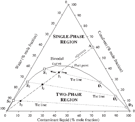
Sample ternary-phase diagram.

Fluid viscosity is an important parameter in governing its flow behavior in a porous medium. As an alcohol-enhanced contaminant mixture migrates through the subsurface and encounters water, the mixture viscosity will change and consequently affects the movement of the contaminant mixture. The mixture viscosity variation is typically neglected in fate and transport mathematical models. This is partly due to the fact that relatively little experimental data are available in literature involving alcohol-enriched contaminant mixtures containing water. In this study, the fluid viscosity variations as water was continuously added to three different predetermined fixed-quantity alcohol-enriched contaminant liquid mixtures (50%–50% by volume) were experimentally measured. Methanol was the cosolvent considered in this study, along with the three aforementioned common subsurface contaminant liquids. A modified falling-ball viscometer was used to determine the viscosity value of each mixture. In the two-phase region, the viscosity of each liquid phase was independently determined by mixing the composition represented by a tie line end point (such as S and D points in Fig. 1). Note that all S and D points lie on the binodal curve. Therefore, the fluid viscosity of each phase in a two-phase liquid–liquid system can be determined if experimental equilibrium-phase separation data and corresponding tie lines are available. Finally, the viscosity model presented by Teja and Rice (1981) was used to compare the experimentally observed viscosities against model-derived viscosities. This model is based on the generalized corresponding states principle, and it has been used successfully for a wide range of fluid mixtures (e.g., Teja and Rice, 1981; Teja et al., 1985; Kouris and Panaylotou, 1989; Liu et al., 1991; Cedeño et al., 2000). It should be noted that the viscosity models available in literature are not designed for the ternary mixtures presented in this study. Nevertheless, we applied this widely used viscosity model as an initial approach.

Materials and Methods

Modified falling-ball viscometer

The viscosity of each mixture was measured with the modified falling-fall viscometer described in the work of Lee (2008b). Figure 2, adopted from the work of Lee (2008b), is a drawing of the modified falling-ball viscometer. The glass tube has an outer diameter of 1.05 cm and a height of 22.2 cm. The falling ball used in all viscosity experiments is a 0.635-cm (1/4 inch)-diameter stainless-steel spherical ball, with a density of 8.02 g/cm³. The glass tube and the stainless-steel ball are commercially available from Gilmont^® Instruments (Barrington, IL). A second metal spherical ball (not supplied by Gilmont Instruments) has a diameter of 0.5 cm and a density of 6.68 g/cm³. A glass cap was used to seal the glass tube after it was filled with the target liquid(s). The viscometer leveling apparatus described in the work of Lee (2008b) was also used; it is critical that the falling-ball viscometer be placed in an exact vertical position for accurate and reproducible experimental results (Feng et al., 2006). For the falling-ball viscometer used in this study, the following equation yields the viscosity of a liquid by observing the descent time of the falling ball to travel a fixed vertical distance of 10 cm (Fig. 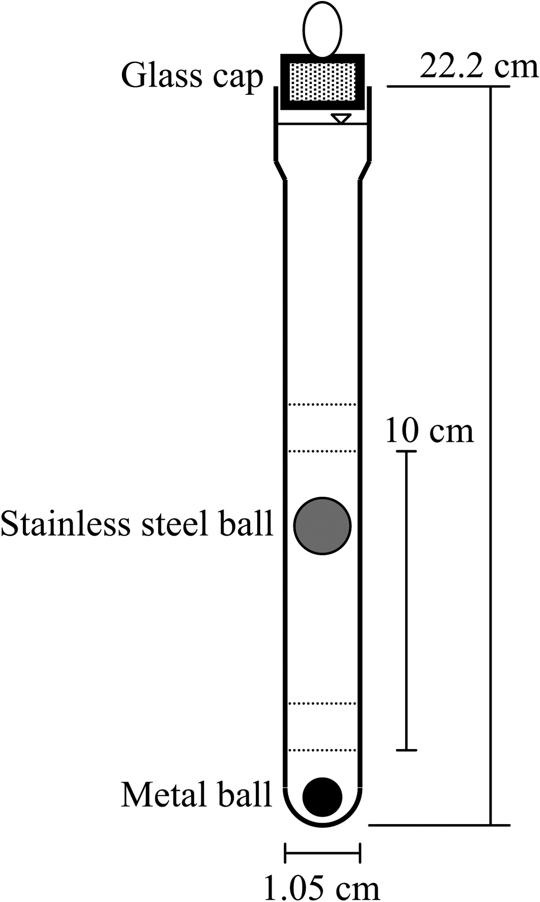2): \documentclass{aastex}\usepackage{amsbsy}\usepackage{amsfonts}\usepackage{amssymb}\usepackage{bm}\usepackage{mathrsfs}\usepackage{pifont}\usepackage{stmaryrd}\usepackage{textcomp}\usepackage{portland, xspace}\usepackage{amsmath, amsxtra}\pagestyle{empty}\DeclareMathSizes{10}{9}{7}{6}\begin{document} \begin{align*} \mu = K (\rho_B - \rho_{FL}) t \tag{1} \end{align*} \end{document}

FIG. 2.

Modified falling-ball viscometer. This figure is not drawn to scale.

where ρ_B is the density of the falling ball, ρ_FL is the density of the liquid, μ is the liquid viscosity (in centipoise [cP]), t is the descent time for the falling ball to travel a fixed vertical distance, and K is the overall viscometer constant. A detailed derivation of eq. (1) can be found in the work of Lee (2008b).

Viscosity experiments

For each viscosity experiment, the glass tube was filled with predetermined amount of target liquid(s) totaling 6.7 mL. Next, the metal ball was inserted into the glass tube, followed by the stainless-steel ball. The glass cap was then immediately placed on top of the glass tube to minimize volatilization. The glass tube was then securely attached to the leveling apparatus. If the target solution contained two or three liquid compounds, an external magnet was used to move the metal ball up and down the glass tube numerous times to assure that the resulting single-phase solution was well mixed. To begin each experiment, the metal ball was moved upward with an external magnet, which also pushed the stainless-steel ball upward. When the stainless-steel ball was near the top of the glass tube (but still in the liquid phase), the magnet was removed, thus allowing both balls to fall downward. Because of the smaller diameter of the metal ball relative to the stainless-steel ball, the metal ball falls to the bottom of the glass tube at a much higher rate relative to the falling rate of the stainless-steel ball. Thus, the addition of the metal ball allowed repeated time-of-descent measurements for the same mixture without flipping over the glass tube. A stopwatch was used to determine the descent time of the stainless-steel ball over a fixed length of 10 cm through the lower half of the viscometer as indicated in Fig. 2. The time-of-descent observations were then repeated for the same mixture until four consistent consecutive falling ball descent times were recorded. The average of the four falling ball descent times was used for liquid viscosity calculation. Next, the glass cap was removed and approximately 2 mL of solution was withdrawn from the glass tube using a 3-mL BD™ disposable syringe with a 1.5-inch needle (www.bd.com). The solution volume within the syringe was determined by reading the syringe markings. The mass of the solution inside the syringe was determined by measuring the difference in syringe mass before and after liquid withdrawal. The density of each target liquid mixture was calculated by dividing the syringe liquid mass by the syringe liquid volume.

Overall viscometer constant

The overall viscometer constant K can be determined from eq. (1) by measuring t for a standard liquid with known viscosity and density values. Using HPLC-grade methanol as the standard liquid, the viscometer constant was determined as K=0.186 cP cm³/(g min). Using this K value, the observed viscosity values for the pure compounds of this study are presented in Table 1. It should be noted that the laboratory temperature was approximately 21°C. Also note that the HPLC-grade methanol and the ACS-grade TCE were obtained from Fisher Scientific (www.fishersci.com). The ACS reagent–grade benzene and the ACS reagent–grade toluene were obtained from the Sigma-Aldrich Company (www.sigmaaldrich.com). Distilled water was used in all experiments when water is a component.

Table 1.

Physical and Chemical Data for Compounds Used in This Study

Compound	Molecular structure	Molecular weight (g/mol)	Published density at 20°C (g/cm ³ )	Published viscosity at 20°C (cP)	Observed viscosity at 21°C (cP)	Viscosity experimental error (%)
Benzene	C₆H₆	78.11	0.8765^a	0.647^a	0.631	2.47
Methanol	CH₄O	32.04	0.791^a	0.583^b	0.583	0
Trichloroethylene	C₂HCl₃	131.39	1.46^a	0.545^c at 25°C	0.556	−2.02
Toluene	C₆H₅CH₃	92.14	0.86^a	0.59^a	0.573	2.88
Water	H₂O	18.02	0.9980^d at 21°C	0.9779^e at 21°C	0.953	2.55

Material safety data sheet.

Kumagai and Yokoyama (1998).

Lide (2004).

Weask (1968).

Weask (1989).

cP, centipoise.

Results and Discussion

Validation of tie line end points (first system)

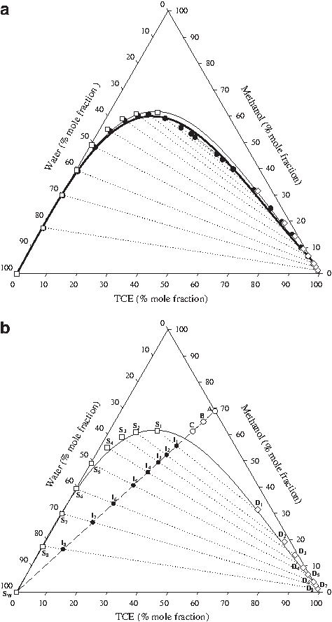
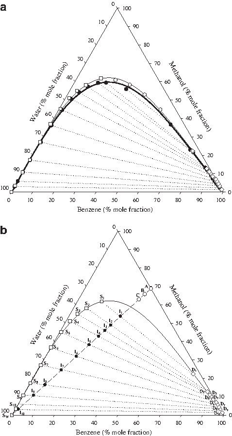
For the first ternary system (methanol, TCE, and water), a set of published experimental equilibrium-phase separation data (black hexagons) along with corresponding tie lines (dotted lines) is shown in Fig. 3a. This set of phase separation data was obtained from the work of Sørensen and Arlt (1979), which were conducted at a temperature of 20°C. The first task of the study was to validate or reestablish the published phase separation data points. This was accomplished by mixing the composition represented by a tie line end point and then visually observing the resulting mixture to determine whether the mixture was a single-phase solution or a two-phase liquid–liquid system (Lee and Ha, 2009). If the resulting mixture for a particular composition was a two-phase liquid–liquid system, then the original published tie line was extended slightly, and a new mixture was prepared along with a new visualization experiment to determine the new tie line end point. The phase visualization experiments were repeated until the resulting mixture was determined a single-phase solution. The phase visualization experiments were repeated for all critical tie line end points. The resulting phase separation data points from this study are also presented in Fig. 3a as white squares and white diamonds. Each white square represents the aqueous phase composition and the corresponding white diamond represents the nonaqueous phase composition. Note that there are two binodal curves generated in Fig. 3a. The thicker binodal curve was generated based on the tie line end points from the Sørensen and Arlt's (1979) dataset (black hexagons), and the thinner binodal curve was generated based on the observed phase separation points from this study (white squares and white diamonds). Each binodal curve was generated using the method described in the work of Lee (2010). It should be noted that all binodal curves in this study were generated using this method. As shown in Fig. 3a, the two binodal curves are similar. Minor differences between the binodal curves may be attributed to factors such as laboratory conditions and/or the quality of the chemical compounds used.

FIG. 3.

(a) Comparison of binodal curves constructed from data observed in this study (thinner curve) and from previously published data (Sørensen and Arlt, 1979) (thicker curve) for a ternary mixture comprised of methanol, trichloroethylene (TCE), and water. (b) The modified ternary-phase diagram along with the dashed line indicating the total composition of the system as water was continuously added to a mixture initially comprising 50% methanol and 50% TCE by volume.

Total composition of the ternary system (first system)

Figure 3b shows the phase separation data points from this study along with modified tie lines based on the Sørensen and Arlt's (1979) dataset. As described earlier, the primary goal of this study was to determine the viscosity variations as water was continuously added to a fixed-quantity cosolvent-contaminant liquid mixture. An initial mixture with volume fractions of 50% methanol and 50% TCE was considered. These volume fractions translated to initial mole fractions of 69.0% methanol and 31.0% TCE, and this composition is indicated on the ternary-phase diagram of Fig. 3b as point A. Note that point A is in the single-phase region and the water mole fraction is at 0%. The dashed line in Fig. 3b represents the changes in total system mole fractions as water was continuously added to this mixture. Note that the mixture partitions into a two-phase liquid–liquid system after the total water mole fraction of the system exceeds approximately 15.3%.

Viscosity and density variations (first system)

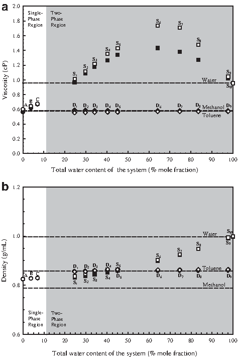
The viscosity of point A and two additional compositions (points B and C in Fig. 3b) within the single-phase region were observed using the modified falling-ball viscometer described earlier. Further, the viscosity values of all composition points indicated by white squares and white diamonds in Fig. 3b were also observed. The observed viscosity values for the first system are presented in Fig. 4a (white symbols). In this figure, the horizontal axis represents the total water content of the system, as represented by the dashed line in Fig. 3b. The unshaded area represents the single-phase region and the shaded area represents the two-phase region. The letter indicators in this figure correspond to the letter indicators in Fig. 3b. For example, point I₁ in Fig. 3b has a total water mole fraction of 19.3%, and at this total water mole fraction, the mixture is a two-phase liquid–liquid system with point S₁ indicating the composition of the aqueous phase and point D₁ indicating the composition of the nonaqueous phase. Therefore, the viscosity values representing points S₁ and D₁ are indicated in Fig. 4a at a total water mole fraction of 19.3%. The viscosity of pure methanol, pure TCE, and water are also plotted (dashed lines) in this figure for comparison. For this system, the observed viscosity of the initial binary mixture (point A) is higher than the viscosity of pure methanol and pure TCE. As water was continuously added to this system, the observed viscosity in the single-phase region (points A, B, and C) increased with increasing water content as indicated in Fig. 4a. At approximately 15.3% total water mole fraction, the mixture partitions into a two-phase liquid–liquid system. In the two-phase region, the viscosity of the aqueous phase (white squares) increased dramatically with increasing total water content, eventually reaching a maximum viscosity near the point S₇, and then the viscosity value decreased with additional water. Note that the point S_w indicates the viscosity of water. It is also interesting to note that all observed aqueous phase viscosity (points S₁ through S₈) are higher than the viscosity of water. The observed nonaqueous phase viscosity (white diamonds) initially decreased with increasing total water content and then remained relatively invariant with additional water.

FIG. 4.

(a) Viscosity and (b) density variations of each liquid phase as water was continuously added to a mixture initially comprising 50% methanol and 50% TCE by volume.

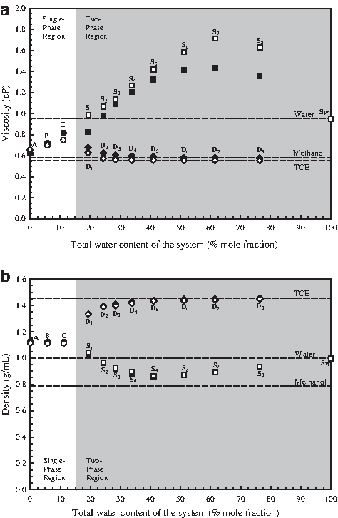
Figure 4b shows the observed density (white symbols) from this study as well as the calculated density (black symbols) based on the following estimation equation: \documentclass{aastex}\usepackage{amsbsy}\usepackage{amsfonts}\usepackage{amssymb}\usepackage{bm}\usepackage{mathrsfs}\usepackage{pifont}\usepackage{stmaryrd}\usepackage{textcomp}\usepackage{portland, xspace}\usepackage{amsmath, amsxtra}\pagestyle{empty}\DeclareMathSizes{10}{9}{7}{6}\begin{document} \begin{align*} \rho_ {\rm Fluid \ Mixture} = \frac {(\rho_1 V_1 + \rho_2 V_2 + \rho_3 V_3)} {( V_1 + V_2 + V_3 )} \tag {2} \end{align*} \end{document}

where ρ₁, ρ₂, ρ₃ are the pure densities for the three liquids, and V₁, V₂, V₃ are the added volumes of the three liquids. The circles represent densities in the single-phase region. In the two-phase region, the squares and diamonds represent the aqueous phase and nonaqueous phase densities, respectively. Each dashed line represents the density of the corresponding pure liquid. Note that the experimentally determined densities are very similar to the estimated densities. In the single-phase region, the density of the mixture remained relatively invariant as more water was added to the system. In the two-phase region, the nonaqueous phase density increased with increasing total water content, whereas the aqueous phase density initially decreased (until near the point S₅) and then increased with increasing total water content.

Second system results

Figure 5a and b follow the same logic and description as Fig. 3a and b, respectively, except that the contaminant liquid is toluene (second system). The equilibrium-phase separation dataset in Fig. 5a (black hexagons) along with corresponding tie lines were obtained from the work of Tamura et al. (2001). Their experiments were conducted at a temperature of 25°C. However, note that the Tamura et al. (2001) dataset does not provide enough data points for accurate modeling of the binodal curve. Therefore, six additional equilibrium-phase separation data points were visually determined in this study. These six data points are presented in Fig. 5a as white hexagons, and they are used for the modeling of both binodal curves. An initial mixture with volume fractions of 50% methanol and 50% toluene was considered. These volume fractions translated to initial mole fractions of 72.6% methanol and 27.4% toluene, as indicated by point A in Fig. 5b. Figure 6a (viscosity variations) and 6b (density variations) follow the same logic and description as Fig. 4a and b. Note that the viscosity variation trend shown in Fig. 6a is similar to that of Fig. 4a. In the single-phase region, the viscosity increased with increasing total water content. At approximately 11.2% total water mole fraction, the solution partitions into a two-phase liquid–liquid system. In the two-phase region, the aqueous phase viscosity (white squares) increased with increasing total water content, reaching a maximum value near point S₆ and then the viscosity decreased with additional water. The nonaqueous phase viscosity (white diamonds) remained relatively invariant with additional water. Figure 6b shows that right after the system transitions from the single-phase region to the two-phase region, the nonaqueous phase density (white diamond) is higher than the aqueous phase density (white square). Thus, the toluene-rich nonaqueous phase will initially form below the aqueous phase. As more water is added to the system, the density of the aqueous phase eventually becomes higher relative to the density of the nonaqueous phase at approximately 45% total system water content. After this total system water content, the nonaqueous phase forms above the aqueous phase.

FIG. 5.

(a) Comparison of binodal curves constructed from data observed in this study (thinner curve) and from previously published data (Tamura et al., 2001) (thicker curve) for a ternary mixture comprised of methanol, toluene, and water. (b) The modified ternary-phase diagram along with the dashed line indicating the total composition of the system as water was continuously added to a mixture initially comprising 50% methanol and 50% toluene by volume.

FIG. 6.

(a) Viscosity and (b) density variations of each liquid phase as water was continuously added to a mixture initially comprising 50% methanol and 50% toluene by volume.

Third system results

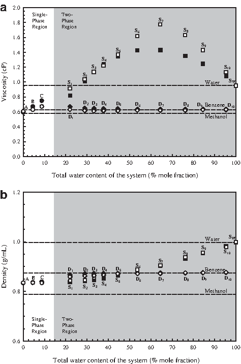
Figure 7a and b also follow the same logic and description as Fig. 3a and b, except that the contaminant liquid is benzene (third system). The phase separation dataset in Fig. 7a (black hexagons) along with corresponding tie lines were obtained from the work of Sørensen and Arlt (1979). Their experiments were conducted at a temperature of 30°C. Again, the thicker binodal curve was generated based on the Sørensen and Arlt's (1979) dataset, and the thinner binodal curve was generated based on the dataset of this study. Note that the Sørensen and Arlt's (1979) dataset contained enough data points covering the entire range of the binodal curve, and thus no additional data points were needed for accurate modeling of the thicker binodal curve. However, four additional equilibrium-phase separation data points (white hexagons) were visually determined in this study to provide a more accurate modeling of the thinner binodal curve. Point A in Fig. 7b represents initial mixture volume fractions of 50% methanol and 50% benzene. Figure 8a (viscosity variations) and 8b (density variations) follow the same logic and description as Fig. 6a and b. Note that both the viscosity and density variations for benzene (Fig. 8) exhibit similar trends compared with that of toluene (Fig. 6).

FIG. 7.

(a) Comparison of binodal curves constructed from data observed in this study (thinner curve) and from previously published data (Sørensen and Arlt, 1979) (thicker curve) for a ternary mixture comprised of methanol, benzene, and water. (b) The modified ternary-phase diagram along with the dashed line indicating the total composition of the system as water was continuously added to a mixture initially comprising 50% methanol and 50% benzene by volume.

FIG. 8.

(a) Viscosity and (b) density variations of each liquid phase as water was continuously added to a mixture initially comprising 50% methanol and 50% benzene by volume.

Viscosity modeling

The viscosity model of Teja and Rice (1981) was used to estimate the viscosity of each mixture. The model is as follows: \documentclass{aastex}\usepackage{amsbsy}\usepackage{amsfonts}\usepackage{amssymb}\usepackage{bm}\usepackage{mathrsfs}\usepackage{pifont}\usepackage{stmaryrd}\usepackage{textcomp}\usepackage{portland, xspace}\usepackage{amsmath, amsxtra}\pagestyle{empty}\DeclareMathSizes{10}{9}{7}{6}\begin{document} \begin{align*} \ln ( \mu \varepsilon ) = \ln ( \mu \varepsilon ) ^ { ( r1 )} + \frac { \omega - \omega^ { ( r1 )}} { \omega^ { ( r2 )} - \omega^ { ( r1 )}} [ \ln ( \mu \varepsilon ) ^ { ( r2 )} - \ln ( \mu \varepsilon ) ^ { ( r1 )} ] \tag {3} \end{align*} \end{document}

where superscripts r1 and r2 refer to the two reference fluids, and the remaining variables in eq. (3) are defined as \documentclass{aastex}\usepackage{amsbsy}\usepackage{amsfonts}\usepackage{amssymb}\usepackage{bm}\usepackage{mathrsfs}\usepackage{pifont}\usepackage{stmaryrd}\usepackage{textcomp}\usepackage{portland, xspace}\usepackage{amsmath, amsxtra}\pagestyle{empty}\DeclareMathSizes{10}{9}{7}{6}\begin{document} \begin{align*} \varepsilon = \frac {V_c^{2 / 3}} {(T_c M)^{1 / 2}} \tag{4} \end{align*} \end{document} \documentclass{aastex}\usepackage{amsbsy}\usepackage{amsfonts}\usepackage{amssymb}\usepackage{bm}\usepackage{mathrsfs}\usepackage{pifont}\usepackage{stmaryrd}\usepackage{textcomp}\usepackage{portland, xspace}\usepackage{amsmath, amsxtra}\pagestyle{empty}\DeclareMathSizes{10}{9}{7}{6}\begin{document} \begin{align*} V_{cm} = \sum\nolimits_i \sum\nolimits_j x_i x_j V_{cij} \tag{5} \end{align*} \end{document} \documentclass{aastex}\usepackage{amsbsy}\usepackage{amsfonts}\usepackage{amssymb}\usepackage{bm}\usepackage{mathrsfs}\usepackage{pifont}\usepackage{stmaryrd}\usepackage{textcomp}\usepackage{portland, xspace}\usepackage{amsmath, amsxtra}\pagestyle{empty}\DeclareMathSizes{10}{9}{7}{6}\begin{document} \begin{align*} T_{cm} = \frac {\sum\nolimits_i \sum\nolimits_j x_i x_j T_{cij} V_{cij}} {V_{cm}} \tag{6} \end{align*} \end{document} \documentclass{aastex}\usepackage{amsbsy}\usepackage{amsfonts}\usepackage{amssymb}\usepackage{bm}\usepackage{mathrsfs}\usepackage{pifont}\usepackage{stmaryrd}\usepackage{textcomp}\usepackage{portland, xspace}\usepackage{amsmath, amsxtra}\pagestyle{empty}\DeclareMathSizes{10}{9}{7}{6}\begin{document} \begin{align*} M_m = \sum\nolimits_i x_i M_i \tag{7} \end{align*} \end{document} \documentclass{aastex}\usepackage{amsbsy}\usepackage{amsfonts}\usepackage{amssymb}\usepackage{bm}\usepackage{mathrsfs}\usepackage{pifont}\usepackage{stmaryrd}\usepackage{textcomp}\usepackage{portland, xspace}\usepackage{amsmath, amsxtra}\pagestyle{empty}\DeclareMathSizes{10}{9}{7}{6}\begin{document} \begin{align*} \omega_m = \sum\nolimits_i x_i \omega_i \tag{8} \end{align*} \end{document} \documentclass{aastex}\usepackage{amsbsy}\usepackage{amsfonts}\usepackage{amssymb}\usepackage{bm}\usepackage{mathrsfs}\usepackage{pifont}\usepackage{stmaryrd}\usepackage{textcomp}\usepackage{portland, xspace}\usepackage{amsmath, amsxtra}\pagestyle{empty}\DeclareMathSizes{10}{9}{7}{6}\begin{document} \begin{align*} V_{cij} = \frac {(V_{ci}^{1/3} + V_{cj}^{1/3})^3} {8} \tag{9} \end{align*} \end{document} \documentclass{aastex}\usepackage{amsbsy}\usepackage{amsfonts}\usepackage{amssymb}\usepackage{bm}\usepackage{mathrsfs}\usepackage{pifont}\usepackage{stmaryrd}\usepackage{textcomp}\usepackage{portland, xspace}\usepackage{amsmath, amsxtra}\pagestyle{empty}\DeclareMathSizes{10}{9}{7}{6}\begin{document} \begin{align*} T_{cij} V_{cij} = \psi_{ij} (T_{ci} T_{cj} V_{ci} V_{cj})^{1/2} \tag{10} \end{align*} \end{document}

where V_c is the critical volume, T_c is the critical temperature, ω is the acentric factor, M is the molecular weight, x is the mole fraction, ψ_ij and is a binary interaction coefficient.

The usage of this model for a ternary mixture requires temperature-dependent viscosity data of two reference liquids (r1 and r2). For the first system, the two selected reference liquids for the single-phase region are methanol and TCE. In the two-phase region, the two selected reference liquids for the aqueous phase are methanol and water, and the two selected reference liquids for the nonaqueous phase are methanol and TCE. For the second system, the two selected reference liquids for the single-phase region are methanol and toluene. In the two-phase region, the two selected reference liquids for the aqueous phase are methanol and water, and the two selected reference liquids for the nonaqueous phase are methanol and toluene. For the third system, the two selected referenced liquids for the single-phase region are methanol and benzene. In the two-phase region, the two selected reference liquids for the aqueous phase are methanol and water, and the two selected reference liquids for the nonaqueous phase are methanol and benzene. It should be noted that the reference liquid viscosities are needed at a temperature equal to T=T₁(T_c/T_cm), where T₁ is the experimental temperature equal to 294.16 K (21°C). To estimate the viscosities of the reference liquids at various temperatures, the method of Lewis-Squires was used (Poling et al., 2000): \documentclass{aastex}\usepackage{amsbsy}\usepackage{amsfonts}\usepackage{amssymb}\usepackage{bm}\usepackage{mathrsfs}\usepackage{pifont}\usepackage{stmaryrd}\usepackage{textcomp}\usepackage{portland, xspace}\usepackage{amsmath, amsxtra}\pagestyle{empty}\DeclareMathSizes{10}{9}{7}{6}\begin{document} \begin{align*} \mu^{- 0.2661} = \mu_K^{- 0.2661} + \frac {T - T_K} {233} \tag {11} \end{align*} \end{document}

where μ_k is the known liquid viscosity at a temperature equal to T_k.

Teja and Rice (1981) reported that the binary interaction coefficient ψ_ij is equal to 1.0 for a mixture of methanol and TCE, 0.99 for methanol and toluene, 1.0 for methanol and benzene, and 1.34 for methanol and water. Note that it is not possible to conduct experiments to determine the binary interaction coefficient for an immiscible binary mixture such as TCE and water. Thus, for the immiscible binary mixtures, a maximum value of 1.37 reported by Teja and Rice (1981) was assumed.

Values of T_c, V_c, and ω for benzene, methanol, toluene, and water were obtained from the work of Poling et al. (2000). For TCE, the values of T_c and V_c were obtained from the work of Dean (1992), and the value of ω was estimated from the following correlation (Lyman et al., 1990): \documentclass{aastex}\usepackage{amsbsy}\usepackage{amsfonts}\usepackage{amssymb}\usepackage{bm}\usepackage{mathrsfs}\usepackage{pifont}\usepackage{stmaryrd}\usepackage{textcomp}\usepackage{portland, xspace}\usepackage{amsmath, amsxtra}\pagestyle{empty}\DeclareMathSizes{10}{9}{7}{6}\begin{document} \begin{align*} \omega = \frac {3} {7} \Big( \frac {T_{br}} {1 - T_{br}} \Big) \log P_c - 1 \tag {12} \end{align*} \end{document}

where T_br=T_b/T_c, T_b is the boiling temperature, and P_c is the critical pressure. For TCE, the value of T_b was obtained from the work of Lide (2004) and the value of P_c was obtained from the work of Dean (1992).

The modeling results are presented in Figs. 4a, 6a, and 8a as black circles in the single-phase region and as black diamonds (nonaqueous phase) and black squares (aqueous phase) in the two-phase region. Note that a similar modeling trend is apparent in all three figures. In the single-phase region, the model shows an increase in viscosity with increasing total water content. In the two-phase region, the Teja and Rice's (1981) model-derived viscosities matched the experimental viscosities fairly well in the nonaqueous phase, and the model was capable of capturing the general viscosity variation trend in the aqueous phase region. To determine the deviation of the model-derived viscosities, the following average absolute deviation (AAD) equation was used: \documentclass{aastex}\usepackage{amsbsy}\usepackage{amsfonts}\usepackage{amssymb}\usepackage{bm}\usepackage{mathrsfs}\usepackage{pifont}\usepackage{stmaryrd}\usepackage{textcomp}\usepackage{portland, xspace}\usepackage{amsmath, amsxtra}\pagestyle{empty}\DeclareMathSizes{10}{9}{7}{6}\begin{document} \begin{align*} {\rm AAD} (\%) = \frac {100} {N} \sum\nolimits_{i = 1}^N \frac {| \mu_{\rm cal} - \mu_{\rm obs}|} {\mu_{\rm obs}} \tag {13} \end{align*} \end{document}

where N is the number of samples, μ_cal is the model-derived viscosity, and μ_obs is the experimentally observed viscosity. For the first system, the calculated AAD for the single-phase region is 2.35%. In the two-phase region, the calculated AADs are 6.20% and 10.63% for the nonaqueous and aqueous phases, respectively. For the second system, the calculated AAD for the single-phase region is 3.26%. In the two-phase region, the calculated AADs are 3.87% and 8.12% for the nonaqueous and aqueous phases, respectively. For the third system, the calculated AAD for the single-phase region is 5.12%. In the two-phase region, the calculated AADs are 3.33% and 7.78% for the nonaqueous and aqueous phases, respectively.

Conclusion

Viscosity experiments were conducted to study the mixture viscosity variations as water was continuously added to a common groundwater liquid contaminant enriched with methanol (50%–50% by volume). Three common groundwater contaminants were considered, namely benzene, toluene, and TCE. Initially, at low water contents, the resulting mixture was a single-phase solution. As the total water content surpassed a critical value, phase separation occurred and the ternary mixture formed a two-phase liquid–liquid system. In the single-phase region, experimental results showed that the mixture viscosity increased with increasing total water content. In the two-phase region, the nonaqueous phase viscosity initially decreased with increasing total water content and then remained relatively invariant as more water was added to the system. The aqueous phase viscosity increased rather significantly with increasing total water content, eventually reaching a maximum value before a decrease in viscosity was observed. The viscosity model presented by Teja and Rice (1981) was used to compare the experimentally observed viscosities against model-derived viscosities. Modeling results showed that the average absolute deviation errors were fairly small in the single-phase region for the three systems considered in this study. In the two-phase region, modeling results showed that the errors were relatively higher in the aqueous phase than in the nonaqueous phase. As viscosity is a key parameter in governing the movement of a fluid in porous media, the variation in mixture viscosities observed in this study emphasizes the need to account for viscosity variability in subsurface contaminant fate and transport mathematical models involving alcohol-enriched contaminant mixtures.

Footnotes

Acknowledgment

This study was partially funded by a grant from the National Science Foundation (0820983).

Author Disclosure Statement

The authors declare that no conflicting financial interests exist.

References

Bao

W.M.J.

, Vogler

E.T.

, Chrysikopoulos

C.V.

2003. Nonaqueous liquid pool dissolution in three-dimensional heterogeneous subsurface formations. Environ. Geol., 43:968.

Brandes

, Farley

K.J.

1993. Importance of phase behavior on the removal of residual DNAPLs from porous media by alcohol flooding. Water Environ. Res., 65:869.

Cedeño

F.O.

, Prieto

M.M.

, Huidobro

J.A.

2000. Viscosities of binary and ternary mixtures of hexadecanoic, octadecanoic, and cis-9-octadecenoic acids. J. Chem. Eng. Data, 45:219.

Chen

C.S.

, Lai

Y.W.

, Tien

C.J.

2008. Partitioning of aromatic and oxygenated constituents into water from regular and ethanol-blended gasolines. Environ. Pollut., 156:988.

Corseuil

H.X.

, Kaipper

B.I.A.

, Fernandes

2004. Cosolvency effect in subsurface systems contaminated with hydrocarbons and ethanol. Water Res., 38:1449.

Dean

J.A.

1992. Lange's Handbook of Chemistry, 4th. New York: McGraw Hill Book Company, Inc.

Falta

R.W.

1998. Using phase diagrams to predict the performance of cosolvent floods for NAPL remediation. Ground Water Monit. Remediat., 18:94.

Falta

R.W.

, Lee

C.M.

, Brame

S.E.

, Roeder

, Coates

J.T.

, Write

, Wood

A.L.

, Enfield

C.G.

1999. Field test of high molecular weight alcohol flushing for subsurface nonaqueous phase liquid remediation. Water Resour. Res., 35:2095.

Feng

, Graham

A.L.

, Abbott

, Mondy

2006. Improving falling ball tests for viscosity determination. J. Fluid Eng., 128:157.

10.

Harmon

T.C.

, Kim

T.J.

, Dela Barre

B. K

, Chrysikopoulos

C.V.

1999. Cosolvent-water displacement in one-dimensional soil columns. J. Environ. Eng. ASCE, 125:87.

11.

Hayden

N.J.

, Diebold

, Noyes

1999. Phase behavior of chlorinated solvent+water+alcohol mixtures with application to alcohol flushing. J. Chem. Eng. Data, 44:1085.

12.

Imhoff

P.T.

, Gleyzer

S.N.

, McBride

J.F.

, Vancho

L.A.

, Okuda

, Miller

C.T.

1995. Cosolvent-enhanced remediation of residual reuse nonaqueous phase liquids: experimental investigation. Environ. Sci. Technol., 29:1966.

13.

Kouris

, Panaylotou

1989. Dynamic viscosity of mixtures of benzene, ethanol, and n-Heptane at 298.15K. J. Chem. Eng. Data, 34:200.

14.

Kumagai

, Yokoyama

1998. Liquid viscosity of binary mixtures of methanol with ethanol and 1-propanol from 273.15 to 333.15 K. Int. J. Thermophys., 19:3.

15.

Lee

K.Y.

2008a. Phase partitioning modeling of ethanol, isopropanol, and methanol with BTEX compounds in water. Environ. Pollut., 154:320.

16.

Lee

K.Y.

2008b. Viscosity off high-alcohol content fuel blends with water: subsurface contaminant transport implications. J. Hazard. Mater., 160:94.

17.

Lee

K.Y.

2010. A model to describe the binodal curve on a type 1 ternary phase diagram. J. Environ. Eng. ASCE, 136:650.

18.

Lee

K.Y.

, Chrysikopoulos

C.V.

2006. Dissolution of a multicomponent DNAPL pool in an experimental aquifer. J. Hazard. Mater., 128:218.

19.

Lee

K.Y.

, Ha

D.T.

2009. Phase separation behavior of three common alcohols with methoxy-nonafluorobutane or ethoxy-nonafluorobutane in water. Can. J. Civil Eng., 36:738.

20.

Lee

K.Y.

, Peters

C.A.

2004. UNIFAC modeling of cosolvent phase partitioning in nonaqueous phase liquid-water systems. J. Environ. Eng. ASCE, 130:478.

21.

Lide

D.R.

2004. CRC Handbook of Chemistry and Physics, 85th. Boca Raton, Florida: CRC Press.

22.

Liu

, Wang

, Chang

C.H.

1991. Model with temperature-independent parameters for the viscosities of liquid mixtures. Ind. Eng. Chem. Res., 30:1617.

23.

Lunn

S.R.D.

, Kueper

B.H.

1997. Removal of pooled dense, nonaqueous phase liquid from saturated porous media using upward gradient alcohol floods. Water Res. Res., 33:2207.

24.

Lyman

W.J.

, Reehl

W.F.

, Rosenblatt

D.H.

1990. Handbook of Chemical Property Estimation Methods. Washington, DC: American Chemical Society.

25.

Peters

C.A.

, Luthy

R.G.

1994. Semiempirical thermodynamic modeling of liquid-liquid phase equilibria: coal tar dissolution in water-miscible solvents. Environ. Sci. Technol., 28:1331.

26.

Poling

B.E.

, Prausnitz

J.M.

, O'Connell

J.P.

2000. The Properties of Gases and Liquids, 5th. New York: McGraw Hill Book Company, Inc.

27.

Sørensen

J.M.

, Arlt

1979. Liquid-Liquid Equilibrium Data Collection, 5. Great Neck, NY: DECHEMA.

28.

Stafford

B.P.

, Cápiro

N.L.

, Alvarez

P.J.J.

, Rixey

W.G.

2009. Pore water characteristics following a release of neat ethanol onto pre-existing NAPL. Ground Water Monit. Remediat., 29:93.

29.

Tamura

, Chen

, Yamada

2001. Ternary and quaternary liquid-liquid equilibria for fuel additives of the water+methanol+toluene and water+methanol+toluene+methyl tert-butyl ether or tert-amyl methyl ether systems at 298.15 K. J. Chem. Eng. Data, 46:1381.

30.

Teja

A.S.

, Rice

1981. Generalized corresponding states method for the viscosities of liquid mixture. Ind. Eng. Chem. Fundam., 20:77.

31.

Teja

A.S.

, Thurner

P.A.

, Pasumarti

1985. Calculation of transport properties of mixtures for synfuels process design. Ing. Eng. Chem. Process Des. Dev., 24:344.

32.

Treybal

R.E.

1963. Liquid Extraction, 2nd. New York: McGraw Hill Book Company, Inc.

33.

Weask

R.C.

1968. CRC Handbook of Chemistry and Physics, 49th. Cleveland, OH: The Chemical Rubber Co.

34.

Weask

R.C.

1989. CRC Handbook of Chemistry and Physics, 70th. Boca Raton, FL: CRC Press.