Hydrological Modeling of Subartic Wetlands: Comparison Between SLURP and WATFLOOD

Abstract

Subarctic wetlands span almost one-sixth of the Canadian wetlands and have been acknowledged as an important ecotone between arctic tundra and boreal forest. Their hydrological complexity is determined by the climatological and physiographical characteristics with regard to the spatiotemporal distribution of water resources. In this study, two semi-distributed hydrological models, SLURP (semi-distributed land use-based runoff processes) and WATFLOOD^™, were employed to understand their effectiveness in modeling the hydrology of subarctic wetlands. Comparisons of their delineation approaches, formulations, parameters, and simulation results indicated that both models were capable of simulating the hydrological processes. However, differences were also observed. Besides their different segment delineation approaches, snowmelt and spring peak flows simulated by SLURP were 4–7 days earlier than those estimated by WATFLOOD because SLURP predefines snowmelt rates as variables, whereas WATFLOOD applies constants in the degree-day method. Due to the lack of considering the existence of permafrost and numerous seasonal ponds, both models tended to underestimate the spring peak flows. Evapotranspiration estimated by the Morton complementary relationship areal evapotranspiration method adopted in SLURP was lower than that calculated by WATFLOOD. Summer runoff only appeared during intense rainfall events, and its concentration was much faster in both models as compared with the observed records, which may be attributed to the variations of permafrost depth, soil water storage capacity, and seasonal pond levels. These findings will be helpful in improving the modeling quality of the two models and understanding the hydrologic features of subarctic wetlands.

Introduction

Wetlands generally include bogs, fens, swamps, marshes, and shallow water where soil is saturated with moisture or inundated by surface or groundwater either permanently or seasonally. Wetlands provide benefits such as wildlife habitats, groundwater reservation, water purification, storage of organic carbon, and adaptation to climatic change (Price et al., 2005). Canada has one-fourth of the world's wetlands and has been divided into seven wetland regions, including arctic, subarctic, boreal, prairie, temperate, oceanic, and mountainous. Among them, subarctic wetlands span almost one-sixth of the Canadian wetlands and have been acknowledged as an important ecotone between arctic tundra and boreal forest. Recently, investigation and conservation of subarctic wetlands has been recognized as an attractive route because of their unique hydrologic features and vulnerability to climate change (Rouse et al., 1997; Woo and Young, 2003; Woo and Thorne, 2006; Ström and Christensen, 2007). Although the hydrology of subarctic wetlands is spatiotemporally complex on account of the shallow ponds and topographical attributes, understanding their hydrologic behaviors is of major concern for the purposes of modeling and predicting how the water cycle may vary in the future (Mansell et al., 2000; Jing et al., 2009).

Semi-distributed hydrological models have been widely used as simplified, conceptual, and mathematical representations of the hydrologic cycle. Unlike lumped conceptual rainfall-runoff models which describe natural environment as a point without any spatial variability, or fully distributed models that always have excessive data demand in grid element scale, semi-distributed hydrological models fit between these two types of models on the basis of a trade-off between process resolution, data availability, and model accuracy. They provide a mechanism for evaluating the impacts of geographical conditions and climatic variations on water resources. The spatial heterogeneity is taken into account by employing various watershed delineation concepts, such as hydrological response unit (HRU) and grouped response unit (GRU) approaches. The HRU approach derives segments from the homogeneity of physiographic and geographic parameters. It has been widely applied with geographic information systems (GIS) and remotely sensed data to facilitate hydrological modeling (See et al., 1992; Greene and Cruise, 1995; Chen, 2007, 2008). Units with similar hydrological response can be grouped by overlying different layers of physiographic information that preserves the heterogeneity of the watershed (Flugel, 1995). Bongartz (2003) stated that the HRU approach can delineate scale-independent homogeneous modeling entities according to spatially distributed physiographical catchment properties. However, it is also sensitive toward variations in land-use change when generating associated runoff. Shaw et al. (2005) claimed that the HRU approach could be impractical for macro-scale basins due to the large amount of segmentation. Hydrological modeling of large basins usually requires distinct hydrological response areas to be grouped within segments. By subdividing a watershed into multiple grid segments, the GRU approach groups of all areas with the similar land cover such that a grid segment may contain a number of distinct GRUs, regardless of location. Hydrological response of each land cover within each grid segment is calculated and then weighted by the fractions of land cover areas (Leon et al., 2001). It allows minority land covers (e.g., marsh, bare soil) to be represented while permitting a large segment that efficiently addresses the problem of computational limitations (Shaw et al., 2005). Kite et al. (1994) applied the GRU approach to simulate the discharge from a 1,600,000 km² watershed by delineating it into only six computational segments. Much discussion on their performance in modeling different watersheds has been continuing in the literature (Filoso et al., 2004; Thompson et al., 2004; Wu and Johnston, 2007; Schmalz et al., 2008; Hattermann et al., 2008).

Many studies have examined the hydrologic features of wetlands using the HRU and GRU approaches (Shaffer et al., 1999; Mansell et al., 2000; Chen et al., 2003; Chen et al., 2004; Price et al., 2005; St Laurent and Valeo, 2007; Hattermann et al., 2008). Nonetheless, such efforts in modeling Canadian subarctic wetland dominated regions have been limited. There are still knowledge gaps in understanding the feasibility and effectiveness in modeling the water cycle of subarctic wetlands and the interactions among hydrological processes, such as snowmelt and spring peak, permafrost and wetland water storage, precipitation intensity and runoff concentration. To better understand the hydrological processes within subarctic wetlands, in this study, the SLURP (semi-distributed land use-based runoff processes) model and the WATFLOOD model were targeted and tested in a Canadian subarctic wetland—the Deer River watershed in northern Manitoba. As two of the major Canadian hydrological models using the HRU and GRU approaches respectively, SLURP and WATFLOOD have been extensively applied in many basins ranging in size from a few hectares to million square kilometres (Haberlandt and Kite, 1998; Fassnacht et al., 1999; Su et al., 2000; Pietroniro et al., 2006; Shin and Kim, 2007; Dibike and Coulibaly, 2007; Armstrong and Martz, 2008; Chen et al., 2010; Jing et al., 2010; Li et al., 2011; Jing and Chen, 2011). However, they have not been parallelly applied in the subarctic region, and their performance in simulating wetland hydrology is still unknown. This study attempts to help fill the above gaps, understand how these two hydrological models, particularly their watershed delineation approaches, would fit the requirements of wetland simulation, and explore their strength and shortcomings in modeling subarctic wetlands.

Study Areas and Field Investigation

The study site—the Deer River watershed is located in north Hudson Bay Lowlands (HBL, 57°55′ N 94°46′ W), 70 km south of Churchill, Manitoba, Canada. It has a drainage area of 5,048 km² with elevations ranging from 16 to 232 m, most of which is covered by tundra, shrub, deciduous, and evergreen forests. The Deer River, as one of the largest tributaries of the Churchill River, originates in the southwest and flows toward the northeast (Fig. 1). The watershed is a broad polygonized peat plateau that consists of high- and low-centered polygons. Volumetric water content of peat soil and hummock is maintained at 60% to 90%. Vegetation is predominantly lichen-heath, in which lichen coverage varies with sub-basins and ranges from 67% to 83% (Wessel and Rouse, 1994; Jing et al., 2009). Deciduous and evergreen forests dominate the headwaters of the Deer River and its downstream channels. The hummocky terrain prevails and consists of porous peat overlying a thick layer of mineral substrate. A great number of seasonal ponds stretch over, whereas continuous permafrost underlies the study area with an active depth of ∼1 m by late August. The primary soils are brunisolic static cryosol, brunisols, brunisolic turbic cryosol, and organo cryosol according to Mills et al. (1976). Mean annual precipitation at nearby Churchill is (1978–2007) 462 mm with maximum in summer (mean July=63 mm; mean August=74 mm; mean September=71 mm), and mean annual temperature is −6.5°C. Winters are long and cold with average temperature varying around −20°C from November to April inclusive. Winter runoff is extremely low and is sustained by groundwater discharge. Snowmelt starts in early or mid May and ceases by the beginning of June, which generates annual peak runoff. Soil water deficits are common in summer and fall due to the intensive evapotranspiration.

FIG. 1.

Location of the Deer River watershed and Chesnaye sub-basin (with monitoring stations).

Due to the limited accessibility of the Deer River watershed, a representative sub-basin in the lower reach of the Deer River, the Chesnaye sub-basin, was selected for modeling parameter investigation during 2006–2008 (Fig. 1). Its elevation slightly varies around 52 m with many seasonally connected ponds stretching over. Vegetation cover is mainly tundra and shrub with little coniferous forest along the streams. The Canada VIA railway goes through the sub-basin from north to south and, thus, provides transportation. A monitoring network of four stream gauging stations (5, 6, 7, 10) and one automated weather station (Rail Spur, 58°09′38″ N 94°08′35.4″ W) was operated during 2006–2008 (Jing, 2009). Data from the weather station were scanned by a Campbell Scientic data logger (model CR1000) and stored as hourly averages. Frost table and surface soil moisture at multiple transects (2, 4, 6 and 8 m away from the bank) of each stream gauging station were measured using steel pole and the SM200 soil moisture sensor. Streamflow was monitored at the gauging stations using HOBO^® water pressure transducer and Sontek^® ADV Flowtracker. Two helicopter trips were also carried out in June and October 2007 to collect information about vegetation coverage, topographic and hydrological conditions across the watershed, and, particularly, in the upper reach of the river.

The 3-year observations at Rail Spur showed a significantly proportional relationship between daily air temperature and evapotranspiration in summer; meanwhile, precipitation played an important role in elevating evapotranspiration with an average lag of 1 day. Soil layers became more saturated as getting closer to the stream channels. On account of the extraordinarily high hydraulic conductivity, locations close to streams received more infiltrated water from streams because the extent of this infiltration process was inversely proportional to distance. After the major recharge period during snowmelt, soil moisture contents kept declining throughout summer, which was mainly due to the intensive evapotranspiration. A reciprocal relationship between the permafrost table and its distance to stream channels was observed. Moreover, the declining trend of permafrost indicated that air temperature acted as the dominant factor of its fluctuation. Most of the small or moderate rainfall events during summer barely generated notable runoff due to the descending frost table, high soil porosity, and intensive evapotranspiration.

Methodology

The SLURP and WATFLOOD hydrological models

The SLURP model version 11 (Kite, 1997) is a semi-distributed, conceptually continuous hydrological model. This daily time-step model was originally developed for meso- and macroscale basins with intermediate complexity, which incorporates necessary physical processes without compromising the simplicity of calculation. It requires the target watershed to be delineated into multiple HRUs—aggregated simulation areas (ASAs) by topographic parameterization. Each ASA is further divided into subareas with different types of land cover based on vegetation, soil, and physiographical conditions. A vertical water balance module is sequentially applied to each type of land cover within each ASA to account for precipitation, canopy interception, snowmelt, infiltration, surface runoff, and groundwater outflow. Precipitation is intercepted by canopy, whereas the amount of precipitation that passes through the canopy is counted as snow or surface storage. Snow melt is calculated using either the degree-day method (Anderson, 1973) or the simplified energy budget method (Kustas et al., 1994). Snowmelt rate is interpolated (parabolically) between the rates in January and July. Infiltration is governed by the Philip formula (Philip, 1954). Three methods from Morton (1983), Spittlehouse (1989), and Granger (1995) are available for estimating evapotranspiration. Surface runoff appears when water remaining in the aerated soil layers after infiltration exceeds the depression storage capacity. Subsurface flow (interflow and groundwater flow) is simulated at a rate depending on subsurface storage and the water transfer coefficient. Manning's equation is applied to route surface and subsurface flow from each land cover to the nearest channel within each ASA. Runoff routing between ASAs is sequentially carried out by using either the hydrological storage techniques or the Muskingum-Cunge channel routing method. Accumulated flow from the outlet of each ASA is routed to the downstream ASA and finally to the outlet of the whole watershed.

WATFLOOD, as a semi-distributed and physically based hydrological model, has been widely used to forecast flood events or simulate watersheds without sacrificing the distributed features and computational efficiency (Kouwen, 2008). As differentiated from SLURP, WATFLOOD is constructed based on the concept of GRUs, which allows its application to large watersheds where similar vegetated areas within each grid segment are grouped as one land cover type for water balance calculation. WATFLOOD allows hourly time increment and simulates both vertical and horizontal water balance in the natural environment, including interception, infiltration, evapotranspiration, snow accumulation and ablation, interflow, recharge, baseflow, and overland and channel routing (Kouwen et al., 1993). Precipitation interception is computed by the Linsley's model (Linsley et al., 1949) with minor changes with regard to the interception evaporation (IET). Snowmelt is estimated by the temperature index routine that allows refreezing (Anderson, 1973) or the radiation temperature index model. In addition, snow sublimation is considered using an adjustable sublimation factor. Potential evapotranspiration (PET) is calculated using either the Priestley-Taylor (Priestly and Taylor, 1972) or the Hargreaves' equation (Hargraeves and Samani, 1982) based on input availability. Actual evapotranspiration (AET) is either presumed as the potential rate when soil moisture is at a level of saturation or reduced to a fraction of the potential rate if soil moisture is below the saturation point. Infiltration process is governed by the Philip formula (Philip, 1954) and the Darcy's law. A ground-water depletion module is applied to diminish base flow. Channel routing is accomplished using the storage routing technique, whereas base flow is calculated by a nonlinear storage-discharge function. Moreover, routing through lakes is available using a used-specified power or polynomial function.

Delineation approach

One of the fundamental differences between SLURP and WATFLOOD is the selection of criteria for watershed discretization. A key question in watershed delineation is to determine what constitutes a hydrological homogeneous area. Usually, answers include the uniformity of physiographic, geographic, and climatological conditions within the target watershed. However, the assumption of uniformity may be violated due to the attempt to maintain a manageable number of segments as the size of the watershed increases. SLURP adopts the HRU approach and delineates a watershed into multiple ASAs based on the homogeneity of physiographic and geographic parameters such that the response to climatic forces would be uniform (Fig. 2a). An HRU can also be arbitrarily defined by land cover, soil type, slope, stream gauges, or even elevation bands. Raster grids that have upstream drainage area larger than the predefined critical source area are determined as the channel network in SLURP. A modification to the channel network is further applied to eliminate any links shorter than the preset minimum source channel length values. A notable advantage of this concept is that its outputs are available in raster format and are able to be compared with satellite-based models. Each ASA is not homogenous and contains multiple land covers with independent flow routing calculations based on their mean distances to the nearest streams. SLURP is capable of recalculating downstream flow values based on transient internal system diversion. However, watershed delineation may not be accurate under some specific topographical conditions, such as board plains where elevation hardly varies. Moreover, it might become difficult when applied to macro-scale basins where a large amount of segmentation could occur in heterogeneous basins.

FIG. 2.

(a) Hydrological response unit (HRU) and (b) grouped response unit (GRU) watershed delineation concept (Donald, 1992).

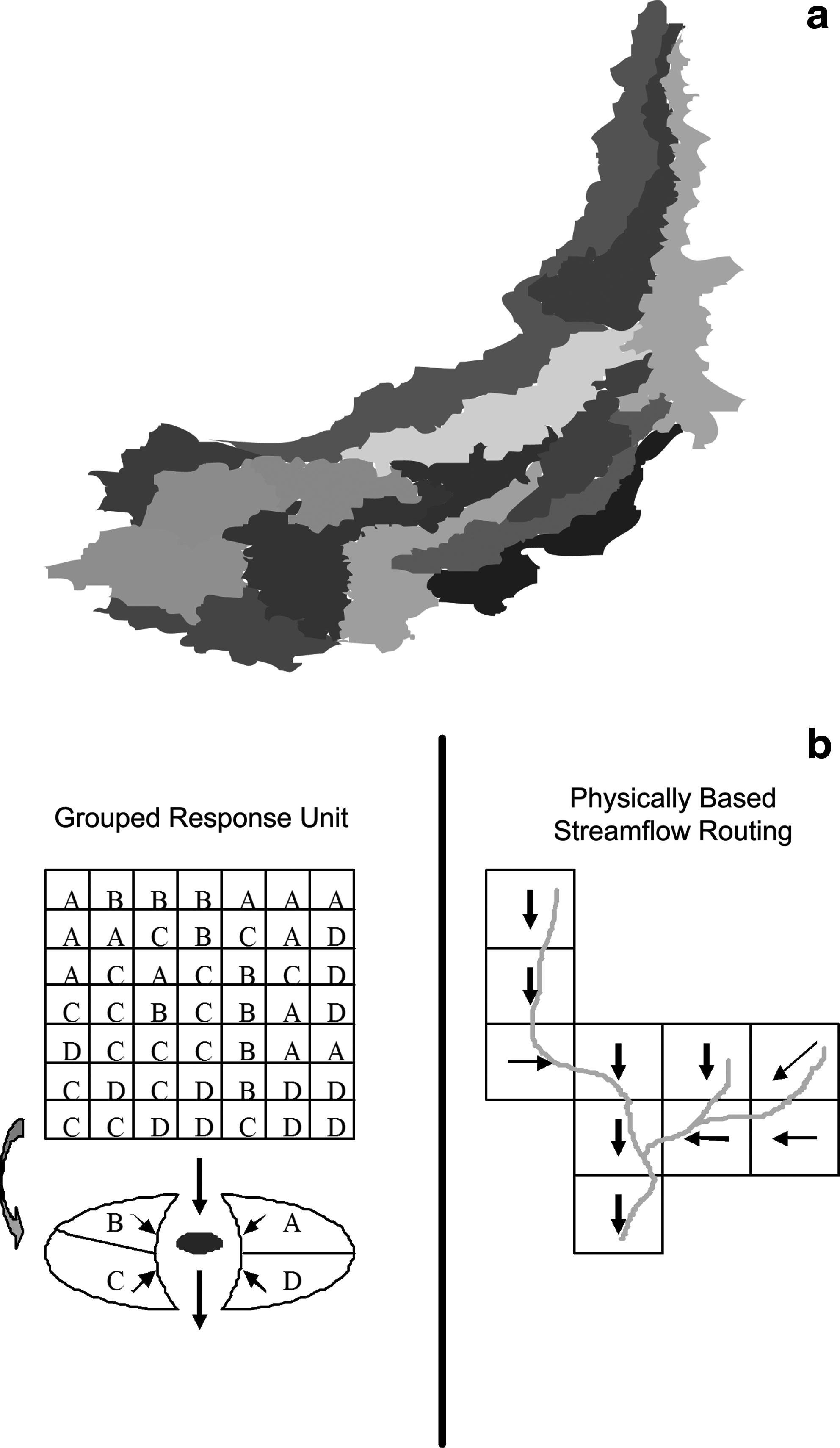
Contrastingly, WATFLOOD employs the GRU approach, which divides the predefined grid segments into a number of distinct GRUs based on their topographic and climatological similarity (Fig. 2b). This approach is ideal to couple to remotely sensed data and GIS. Each segment has identical digital elevation model grids and various land covers with determined ratios, because different types of land cover can have a wide range of response characteristics. The GRU approach calculates the response for each land cover within each segment using standard distributed modeling techniques and, subsequently, weights the response by land cover area fractions. The results from each land cover are then summed to determine the response of each gird segment and the basin. The GRU approach is significantly based on the percentage of each land cover within each grid segment rather than their location. In addition, it is less data-intensive and more efficient than the HRU approach over large spatial scales. These features allow the size of grid units to be determined by a size where routing time within the units are much shorter than the overall basin routing time. Another prominent advantage of the GRU approach is that it can incorporate necessary hydrological features without compromising the simplicity of computation and introducing uncertainties caused by watershed delineation. Additionally, increasing the size of grid segments can remarkably reduce computation and input parameterization effort. However, an inherent weakness of this concept is that heterogeneity may be lost, and only land covers differentiation within one grid could be derived. Moreover, determination of flow direction may also be inaccurate if grid size is too large.

Snowmelt

Snowmelt is defined as surface runoff produced from melting snow in spring and is usually an important fraction of the annual water cycle in subarctic wetlands. The rate of snowmelt is determined by the amount of energy available to the snowpack and is usually dominated by net radiation. Cold snowpack has negative energy balance, whereas warming results in the isothermal condition and additional energy starts the melt. The most commonly used snowmelt-runoff model is the degree-day method or temperature index routine, (Anderson, 1973) which has been successfully verified worldwide over a number of basins and climates. Due to the lack of net radiation data, it was selected for both models. Although this method has inadequate accuracy in simulating small-scale snowmelt rates, it does produce acceptable results at basin scale (Pohl et al., 2005). SLURP uses an increasing parabolic interpolation from values specified in January and July to determine the degree-day factor (Table 1). The later the date is, the greater melt rate. WATFLOOD models snow-free and snow-covered area separately. Although the temperature index routine may not be effective for hourly time increments as the melting process is mainly controlled by radiation (Rango and Martinec, 1995), recent studies reported good modeling results using this routine (Donald, 1992; Seglenieks, 1994; Hamlin, 1996). The degree-day factors of each land cover are calibrated as constants in WATFLOOD in reference to Kouwen (2008) and Stadnyk (2008) (i.e., 0.13–0.17 mm/day/°C). This difference, if under the same ambient conditions (e.g., date, time, temperature, and radiation) in the melting season (April-June), may result in more rapid snow depletion in SLURP.

Table 1.

Summary and Comparisons of the General Characteristics of SLURP and WATFLOOD

	SLURP	WATFLOOD
Delineation approach	HRU	GRU
Snowmelt (Anderson, 1973)	S_m=R₁(T-T_critical) \documentclass{aastex}\usepackage{amsbsy}\usepackage{amsfonts}\usepackage{amssymb}\usepackage{bm}\usepackage{mathrsfs}\usepackage{pifont}\usepackage{stmaryrd}\usepackage{textcomp}\usepackage{portland,xspace}\usepackage{amsmath,amsxtra}\pagestyle{empty}\DeclareMathSizes{10}{9}{7}{6}\begin{document}$$R_1 = [(a - b) \times d^2 + 367 (a - b) \times d] / 33306 + (92a - b) / 91$$\end{document}	S_m=R₁(T−T_critical)R₁ is set to constant for each land cover
Evapotranspiration (Hargraeves and Samani, 1982; Morton, 1983)	\documentclass{aastex}\usepackage{amsbsy}\usepackage{amsfonts}\usepackage{amssymb}\usepackage{bm}\usepackage{mathrsfs}\usepackage{pifont}\usepackage{stmaryrd}\usepackage{textcomp}\usepackage{portland,xspace}\usepackage{amsmath,amsxtra}\pagestyle{empty}\DeclareMathSizes{10}{9}{7}{6}\begin{document}$$AET = 2WEE - PET = \frac {s [(2 \alpha - 1) R_n + 2 \alpha M] - \gamma f_A (e_a^* - e_a)} {\lambda (s + \gamma)}$$\end{document}	\documentclass{aastex}\usepackage{amsbsy}\usepackage{amsfonts}\usepackage{amssymb}\usepackage{bm}\usepackage{mathrsfs}\usepackage{pifont}\usepackage{stmaryrd}\usepackage{textcomp}\usepackage{portland,xspace}\usepackage{amsmath,amsxtra}\pagestyle{empty}\DeclareMathSizes{10}{9}{7}{6}\begin{document}$$PET = 0.0075 \times R_a \times C_t \times \delta_t^{1 / 2} \times T_{avg.d}$$\end{document} \documentclass{aastex}\usepackage{amsbsy}\usepackage{amsfonts}\usepackage{amssymb}\usepackage{bm}\usepackage{mathrsfs}\usepackage{pifont}\usepackage{stmaryrd}\usepackage{textcomp}\usepackage{portland,xspace}\usepackage{amsmath,amsxtra}\pagestyle{empty}\DeclareMathSizes{10}{9}{7}{6}\begin{document}$$AET = PET \cdot UZSI \cdot FPET 2 \cdot FTALL \cdot ETP$$\end{document}
Rainfall-runoff response (days)	Mean: 1.44; Max: 3; Min: 1	Mean: 1.84; Max: 3; Min: 1

Variables are defined in the Notation.

SLURP, semi-distributed land use-based runoff processes; HRU, hydrological response unit; GRU, grouped response unit.

Evapotranspiration

Evapotranspiration is defined as the sum of vaporization from both vegetations and open water bodies, and plant transpiration. It is affected by a number of factors, including vegetation growth stage and maturity, percentage of soil cover, soil moisture, solar radiation, humidity, air temperature, and wind speed. The Penman equation has been widely used to estimate PET, which specifies the maximum evapotranspiration capacity if there were abundant water available (Penman, 1948). However, PET is a theoretical concept and is unlikely to be achieved in most scenarios. Many hydrological models calculate AET from reducing PET, because some water will be lost due to infiltration and surface runoff.

In this study, the Morton complementary relationship areal evapotranspiration (CRAE) model was selected to calculate AET in SLURP (Morton, 1983) due to the lack of sunshine hours and soil heat flux data. As a modification of the Penman equation, it computes PET by replacing the wind function with a vapor transfer coefficient to solve the energy balance and aerodynamic equations. Wet-environment evaporation is derived from an empirical estimation with regard to saturation vapor pressure, temperature curve, and net radiation. AET is computed from a complementary relationship as shown in Table 1. This method has wide appeal, because it does not require many parameters that may affect evapotranspiration and recognizes that AET is often less than PET. However, soil moisture feedback is not included and AET needs to be set to zero if surface and soil water storage depletes. In addition, this method is not land cover dependent.

In the absence of hourly radiation data, the Hargreaves equation was applied in WATFLOOD to empirically estimate PET from daily air temperature (Table 1). Solar input (R_a) is simplified as a function of latitude and Julian day, whereas C_t is regressed from measurements of relative humidity made in the United States (Kouwen, 2008). It is a lumped empirical estimation that may not accurately reflect the real conditions depending on the location of the study area. Nonetheless, this equation consistently produces accurate evapotranspiration approximations in an increasing number of documented studies in spite of not considering dewpoint temperature, vapor pressure, and wind conditions (Hargraeves and Samani, 1982; Mohan, 1991). PET is then further reduced to AET by applying soil moisture (UZSI) and temperature (FPET2), vegetation (FTALL), and peat layer effect (ETP) coefficients when IET is equal to zero. If IET is greater than zero, AET is further adjusted based on the difference between values of PET and IET. This reduction approach appears to be promising, because it addresses the feedback of soil moisture and land cover effects. In spite of this, more specific coefficients may raise the challenges of data input and quality, because they have to be either measured or calibrated.

Modeling input

A 3-arc-second (90 m resolution) digital elevation model of the Deer River watershed was obtained from the National Map Seamless Server of U.S. Geological Survey (USGS, 2008). The study area was delineated into 206 ASAs in SLURP and 54 × 48 square grids in WATFLOOD. Land cover datasets (1 km resolution) were obtained from the Systeme Probatoire d'Observation dela Tarre earth observation satellite system (SPOT IMAGE and VITO, 2008) and reclassified into six land cover classes, including water, impervious, marsh, shrub, coniferous trees, and deciduous trees (Table 2) based on some previous studies in Canadian subarctic region (Stow et al., 2004; St Laurent and Valeo, 2007). Historical streamflow data (1978–1997) were obtained from Water Survey Canada and further compared with modeling outputs at the D. River N. Belcher station (58°0′48″ N 94°11′53″ W, ID: 06FD002, Fig. 1). Meteorological data (1978–1997) at the Churchill-A Climate Station (ID 5060600) were provided by Environment Canada.

Table 2.

Optimized Criterion for Land-Cover Classification

Land covers	NDVI lower bound	NDVI upper bound
Water	0.05	0.20
Impervious	0.20	0.30
Marsh	0.30	0.50
Shrub	0.50	0.54
Coniferous	0.54	0.62
Deciduous	0.62	0.72

Sensitivity analysis

To understand which parameters contribute most to the output, sensitivity analysis was conducted for SLURP and WATFLOOD by adjusting all the model parameters (one-factor-at-a-time) and evaluating their impacts on modeling results. The base values of these parameters were determined in reference to the field investigation in the Chesnaye sub-basin, manuals of both models, and other researchers' work in the HBL where the study area is located (Kite, 1997; Su et al., 2000; Metcalfe and Buttle, 2001; Kite, 2002; Thorne, 2004; Woo and Thorne, 2006). Based on the assumption of independent interrelationship, each parameter was individually adjusted by ±5%, ±15%, and ±30% while keeping all other ones at their initial values (adjustment of each parameter was made to all land covers at one time), and evaluated by the fluctuation of the 10-year (1978–1987) logarithmic Nash and Sutcliffe efficiency (NSE_In) and the correlation coefficient (R) to derive a limited number of influential ones. The 10-year NSE_In and R were calculated by the following equations: \documentclass{aastex}\usepackage{amsbsy}\usepackage{amsfonts}\usepackage{amssymb}\usepackage{bm}\usepackage{mathrsfs}\usepackage{pifont}\usepackage{stmaryrd}\usepackage{textcomp}\usepackage{portland,xspace}\usepackage{amsmath,amsxtra}\pagestyle{empty}\DeclareMathSizes{10}{9}{7}{6}\begin{document}\begin{align*} NSE_{ln} = 1 - \frac {\mathop\sum \limits_{i = 1}^N (lnQ_i - lnQ_m)^2} {\mathop\sum \limits_{i = 1}^N (lnQ_i - lnQ_{ average})^2} \tag {1} \end{align*}\end{document} \documentclass{aastex}\usepackage{amsbsy}\usepackage{amsfonts}\usepackage{amssymb}\usepackage{bm}\usepackage{mathrsfs}\usepackage{pifont}\usepackage{stmaryrd}\usepackage{textcomp}\usepackage{portland,xspace}\usepackage{amsmath,amsxtra}\pagestyle{empty}\DeclareMathSizes{10}{9}{7}{6}\begin{document}\begin{align*} R = \frac {\frac {1} {N} \times \mathop\sum \limits_{i = 1}^N (Q_i - Q_{average}) \times (Q_m - Q_{average})} {\sqrt {\frac {N \times \mathop\sum \limits_{i = 1}^N Q_i^2 - \left(\mathop\sum \limits_{i = 1}^N Q_i \right)^2} {N \times (N - 1)}} \times \sqrt {\frac {N \times \mathop\sum \limits_{i = 1}^N Q_m^2 - \left(\mathop\sum \limits_{i = 1}^N Q_m \right)^2} {N \times (N - 1)}}} \tag {2} \end{align*}\end{document}

where N is the number of days; Q_i is the daily observed flow in 10 years (m³/s); Q_m is the daily modeled flow in 10 years (m³/s); and Q_average is the 10-year mean observed flow (m³/s). The NSE_ln describes model performance in the case of discharge simulations during low-flow periods. The closer it is to 1, the better the performance of the model. The R statistic describes the degree of colinearity between observed and modeled flow. It tends to the unity the more simulated flows have the similar dynamics as observations. The most sensitive parameters to be calibrated in SLURP are initial contents of snow store and slow store, maximum infiltration rate, retention constants for fast store and slow store, maximum capacity for fast store and slow store, precipitation factor, rain/snow division temperature, and snowmelt rates in January and July. Contrastingly, the most influential parameters in WATFLOOD include lower zone drainage function exponent, base temperature for snowmelt, porosity of the wetland or channel bank, reduction in soil evaporation due to tall vegetation, crude snow sublimation factor, melt factor, and manning's roughness coefficient.

Modeling validation

To minimize the difference between observed and simulated runoff rates and compensate for errors in measurement, a 10-year (1978–1987) calibration was conducted for the influential parameters in SLURP and WATFLOOD using their built-in optimization modules and manual adjustment. Both the NSE_ln criterion and the correlation coefficient (R) were used as statistical measures of the goodness of fit of the calibration results at the D. River N. Belcher station. Tables 3 and 4 summarize the final values of model parameters obtained after the calibration of SLURP and WATFLOOD, respectively. Modeling verification was performed for the next 10-year period (1988–1997) to ensure both models accurately reflect the hydrological features of the study area. Tables 5 and 6 show the models' outputs and performance measures using parameters declared in Tables 3 and 4.

Table 3.

Calibrated SLURP Parameters for Each Type of Land Cover in Deer River Watershed

Parameters	Unit	Water	Impervious	Marsh	Shrub	Coniferous	Deciduous
Initial contents of snow store	(mm)	1	1	1	1	1	1
Initial contents of slow store	(%)	9.775	8.625	4.238	6.839	5.895	6.205
Maximum infiltration rate	(mm/day)	100.9	142.4	106.9	147.7	111.9	105.7
Manning roughness n	(dimensionless)	0.02	0.08	0.01	0.07	0.02	0.03
Retention constant for fast store	(day)	36.97	52.62	5.447	7.480	62.89	40.45
Maximum capacity for fast store	(mm)	95.35	133.8	531.2	583.6	373.7	697.0
Retention constant for slow store	(day)	130.7	171.0	686.1	745.5	713.0	747.1
Maximum capacity for slow store	(mm)	338.7	260.6	361.6	102.9	62.19	63.22
Precipitation factor	(dimensionless)	1	1	1	1	1	1
Rain/snow division temperature	(°C)	−0.03	−0.56	−0.99	−0.93	−0.61	−0.32
Canopy interception A	(dimensionless)	0	0.5	1	1	1	1
Canopy interception B	(dimensionless)	1	1	1	1	1	1
Land cover albedo	(dimensionless)	0	0.15	0.15	0.14	0.13	0.16
LAI in January	(dimensionless)	0	0	2	0.5	5	3
LAI in July	(dimensionless)	0	2	2	4.5	5	10
Maximum canopy capacity	(dimensionless)	0	2.8	3.8	6.2	5.6	4.3
Soil heat flux amplitude	(dimensionless)	0.15	0.15	0.15	0.15	0.15	0.15
Snowmelt rate in January	(mm/°C/day)	0	0	0	0	0	0
Snowmelt rate in July	(mm/°C/day)	4	4	4	3	2	2
Maximum albedo of snow	(dimensionless)	0.78	0.78	0.78	0.7	0.7	0.7
Minimum albedo of snow	(dimensionless)	0.37	0.37	0.37	0.37	0.37	0.37
Temperature lapse rate	(°C/100 m)	0.75	0.75	0.75	0.75	0.75	0.75

Table 4.

Calibrated WATFLOOD Parameters for Each Type of Land Cover in Deer River Watershed

Parameter	Description and unit	Deciduous	Coniferous	Shrub	Marsh	Water	Impervious
AK2	Upper zone drainage resistance factor (dimensionless)	0.55	0.55	0.55	0.55	0.051	5E-10
AK2FS	Snow upper zone drainage resistance factor (dimensionless)	0.52	0.51	0.52	0.52	0.051	5E-10
AK	Soil permeability of bare ground (mm/h)	13.4	12	3	400	−0.1	0.1E-10
AKFS	Soil permeability under snow (mm/h)	1.2	1.2	3	400	−0.1	0.1E-10
Albedo	The all-wave albedo (dimensionless)	0.16	0.13	0.14	0.15	0	0.15
BASE	Base temp for snowmelt (°C)	−0.32	−0.61	−0.93	−0.99	−0.03	−0.56
MF	Melt factor (mm/°C/h)	0.13	0.13	0.17	0.17	0.13	0.15
NMF	Negative melt factor (mm/°C/day)	0.10	0.10	0.10	0.10	0.10	0.10
R3	Overland flow roughness for bare area (dimensionless)	0.10	0.08	0.20	0.09	0.04	4
R3FS	Overland flow roughness for snow area (dimensionless)	0.1	0.05	0.20	0.10	0.04	4
REC	Interflow depletion coefficient (dimensionless)	0.2	0.2	0.2	0.9	0.1	0.9
RETN	Upper zone specific retention (mm)	150	150	150	140	0.1	0.1
A5	API hourly reduction value (dimensionless)	0.985	0.985	0.985	0.985	0.985	0.985
Lzf	Lower zone drainage function parameter (dimensionless)	0.1E-4	0.1E-4	0.1E-4	0.1E-4	0.1E-4	0.1E-4
Pwr	Lower zone drainage function exponent (dimensionless)	2.05	2.05	2.05	2.05	2.05	2.05
R2n	Channel Manning's roughness coefficient (dimensionless)	0.018	0.018	0.018	0.018	0.018	0.018
Ds	Depression storage for bare ground (mm)	123	120	1.2E4	1.2E10	0	1
Dsfs	Depression storage for snow covered ground (mm)	223	220	220	2.2E10	0	1
Flapse	Lapse rate in °C per 100m (°C)	0.75	0.75	0.75	0.75	0.75	0.75
Fpet	IET increase for tall vegetation (dimensionless)	3	4	4	4	1	0
Ftal	Soil evaporation reduction of tall vegetation (dimensionless)	0.85	0.85	1	1.3	1	1
Kcond	Conductivity of the wetland (mm/h)	0.75	0.75	0.75	0.75	0.75	0.75
Mndr	Meandering factor (dimensionless)	1	1	1	1	1	1
R1n	Flood plain Manning's roughness coefficient (dimensionless)	0.05	0.05	0.05	0.05	0.05	0.05
Sublime	Crude snow sublimation factor (mm/h)	0.10	0.10	0.22	0.22	0.30	0
Theta	Porosity of the wetland or channel (dimensionless)	0.7	0.7	0.7	0.7	0.7	0.7

Table 5.

Annual Modeling Outputs of SLURP at D. River N. Belcher Station (1978–1997)

Year	Cumulative precipitation (mm)	Mean air temperature (°C)	Cumulative simulated AET (mm)	Mean observed flow (m ³ /s)	Mean simulated flow (m ³ /s)	NSE_ln (%)	R
1978	532.8	−7.76	218.7	12.7	14.6	71	0.74
1979	341.9	−7.96	194.6	13.9	9.9	51	0.89
1980	484.0	−6.93	242.3	18.4	12.4	71	0.82
1981	395.4	−4.89	203.1	14.4	17.9	61	0.84
1982	605.8	−8.43	239.6	15.8	24.6	41	0.86
1983	621.0	−7.06	248.6	27.9	35.7	68	0.69
1984	413.9	−6.50	195.0	14.3	17.8	43	0.65
1985	448.5	−7.11	184.4	11.1	17.0	38	0.65
1986	500.3	−7.33	241.0	22.8	25.6	57	0.92
1987	432.7	−5.42	227.1	11.6	17.1	42	0.77
1988	441.3	−7.38	180.2	9.07	6.68	72	0.92
1989	358.5	−8.02	172.6	17.6	15.8	70	0.61
1990	485.3	−7.41	187.4	12.1	16.4	22	0.74
1991	524.9	−7.09	202.0	23.8	28.6	62	0.93
1992	402.0	−8.21	169.3	12.8	23.1	15	0.78
1993	291.5	−7.11	177.6	9.0	10.4	13	0.63
1994	345.5	−6.62	147.4	7.2	14.0	21	0.51
1995	416.4	−6.90	224.1	19.4	17.2	59	0.88
1996	424.1	−7.46	200.7	7.0	12.7	25	0.86
1997	509.7	−6.55	185.4	27.2	22.1	68	0.94
Average	448.8	−7.1	202.1	15.4	18.0	49	0.78

AET, actual evapotranspiration.

Table 6.

Annual Modeling Outputs of WATFLOOD at D. River N. Belcher Station (1978–1997)

Year	Cumulative precipitation (mm)	Mean air temperature (°C)	Cumulative simulated AET (mm)	Mean observed flow (m ³ /s)	Mean simulated flow (m ³ /s)	NSE_ln (%)	R
1978	532.8	−7.76	403.9	12.7	24.5	8	0.38
1979	341.9	−7.96	204.4	13.9	17.0	41	0.86
1980	484.0	−6.93	332.2	18.4	13.7	66	0.70
1981	395.4	−4.89	325.2	14.4	22.5	38	0.53
1982	605.8	−8.43	527.3	15.8	35.0	20	0.82
1983	621.0	−7.06	610.2	27.9	49.6	36	0.46
1984	413.9	−6.50	235.7	14.3	26.5	20	0.49
1985	448.5	−7.11	325.4	11.1	15.4	28	0.47
1986	500.3	−7.33	431.4	22.8	30.8	49	0.74
1987	432.7	−5.42	299.6	11.6	22.5	25	0.48
1988	441.3	−7.38	207.9	9.07	13.3	48	0.56
1989	358.5	−8.02	232.9	17.6	16.6	58	0.26
1990	485.3	−7.41	320.4	12.1	15.6	41	0.77
1991	524.9	−7.09	419.9	23.8	24.5	55	0.82
1992	402.0	−8.21	401.8	12.8	26.4	13	0.57
1993	291.5	−7.11	135.1	9.0	9.9	25	0.81
1994	345.5	−6.62	186.3	7.2	6.0	52	0.95
1995	416.4	−6.90	397.3	19.4	22.4	52	0.59
1996	424.1	−7.46	233.1	7.0	16.9	7	0.72
1997	509.7	−6.55	462.5	27.2	27.8	68	0.87
Average	448.8	−7.1	334.6	15.4	21.8	38	0.64

Results and Discussion

The first year of a simulation period is an initialization period due to the uncertainty of the initial values for snow cover and water storages. This explains the low NSE_In value (8%) of WATFLOOD in the calibration year 1978 with regard to the lack of initial water storage settings. On the other hand, SLURP utilizes and optimizes specific parameters for initial water storage, which, therefore, enables a good fit between simulated and observed hydrographs in the start year.

SLURP and WATFLOOD allowed fair reproduction of runoff generation dynamics during both high- and low-flow periods. They were able to capture the subarctic wetland character of the discharge regime of the Deer River, governed by snow accumulation and low flow in winter, by typical snowmelt runoff peak in spring, and by intensive evapotranspiration as well as soil water deficit in summer. Application of SLURP to the study area in 1988 resulted in an NSE_In of 72% and an R of 0.92, whereas WATFLOOD produced an NSE_In of 48% and an R of 0.56. The year 1988 was selected as an example, because it was a median year from a meteorological perspective (Table 5). Of the deficiency in NSE_ln, the majority was attributed to simulation during spring snowmelt and summer, whereas the minority was contributed during fall and winter. Overall, SLURP had better performance than WATFLOOD, which might be attributed to the differences in snowmelt and evapotranspiration, as well as model complexities.

Snowmelt runoff

In subarctic wetlands, snowmelt runoff usually commences in May with an increase in runoff during the melting period corresponding to the saturation of organic soil layers and a sharp decline after the snow disappearance. Fluctuations of melt rate exist due to the varying rhythm of melt responding to the seasonal trend. Saturation begins 12–18 days after the start of snowmelt infiltration, indicating most of the snowmelt peaks occur in May or June and lead to pronounced flow maxima in streams. Van der Linden and Woo (2003) applied SLURP to a typical subarctic catchment, the Liard basin in northwest Canada, and reported spring peak flows in early June. Similar trends were observed by other studies conducted in subarctic wetlands (Woo et al., 2000; Carey and Woo, 2001).

Figure 3a shows the Julian days of observed and simulated snowmelt peaks at the D. River N. Belcher station. It can be concluded that most of the simulated peaks were 2–11 days later than observed records. This can probably be explained by the existence of permafrost that blocked the percolation of water and, therefore, increased observed runoffs. In spring, when the permafrost layer is shallow, meltwater could infiltrate the surface porous soil; however, infiltration is retarded by permafrost and a perched saturated zone is formed toward the ground surface to produce continuous lateral runoff (Carey and Woo, 2001). These effects are not considered in either SLURP or WATFLOOD, and meltwater is routed to interflow and groundwater instead of being discharged as instant runoff. Therefore, the modeling results implied a number of days' delay to convey meltwater from snow cover to surface runoff. Another interesting finding was that peaks modeled by SLURP were ∼8 days earlier than those modeled by WATFLOOD. Snowmelt base temperatures were calibrated in both models, and their values were close to each other. Instead of having preset melt rates as in WATFLOOD, SLURP employs parabolically increasing melt factors that might intensify the melt process and result in earlier peaks.

FIG. 3.

(a) Days of observed and simulated snowmelt peaks and (b) observed and simulated snowmelt peak flows at the D. River N. Belcher station (1978–1997).

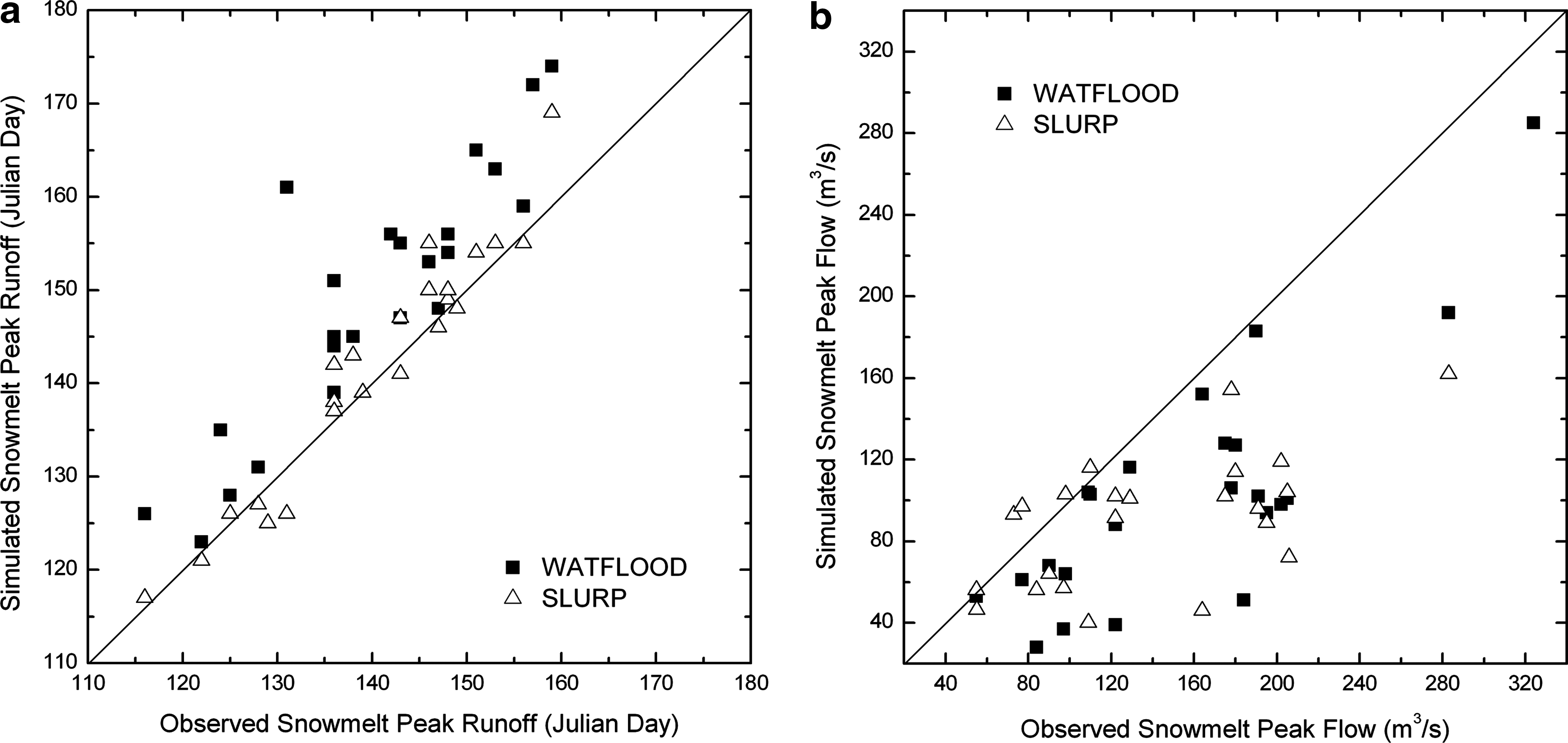
The simulation results also demonstrated that the amount of peak flows was 30% less than the historical records (Fig. 3b). Permafrost represents an over-winter surface storage of groundwater. When temperature increases and snow starts to melt, water is also released as stream runoff from the thaw of ice contents within the organic soil layers (Woo and Thorne, 2006). The numerous seasonal ponds may also contribute to melt peaks, because they have a vast water equivalent storage capacity that can be discharged when air temperature rises. In addition, from the hydrological point of view, permafrost and a discontinuity in the soil properties restrict water percolation and, therefore, excludes the effects of soil water storage. However, meltwater could be intercepted as surface and groundwater storage in both models, resulting in alleviated spring peaks compared with observed records.

Evapotranspiration

The average annual AET estimated by SLURP and WATFLOOD during the modeling period were 202.1 and 334.6 mm, respectively. Rouse (1998) estimated the water balance of a hummocky sedge fen in northern HBL and reported an annual AET rate of 269 mm. Figure 4 shows the temporal trends in observed annual runoff at the D. River N. Belcher station and cumulative AET modeled by the Morton CRAE method in SLURP, the Hargreaves equation WATFLOOD, and Rouse (1998). It can be concluded that SLURP may underestimate AET, whereas WATFLOOD may overestimate it. Summertime AET estimated by the Hargreaves equation was dramatically higher than that from the Morton CRAE method. Take August 1995 as an example, the monthly cumulative AET were 128 and 51 mm for WATFLOOD and SLURP, respectively. This difference may be attributed to a number of possible reasons. First, inputs for PET computations were not the same. SLURP uses a modified version of the Penman equation, whereas WATFLOOD only estimates by temperature, location on the earth, and the Julian day. Second, PET calculated by both models may be subject to inaccuracy due to the lack of applications and experiences in subarctic wetlands, such as the lack of soil wilting points, soil water contents, net radian flux, water depth in the canopy, and saturated vapor pressure. Third, the reduction rates of PET in both models were different. WATFLOOD appears to have a more realistic concept, because it employs soil moisture feedback and land-cover effects. However, these extra factors may cause arbitrary uncertainties during the calibration process.

FIG. 4.

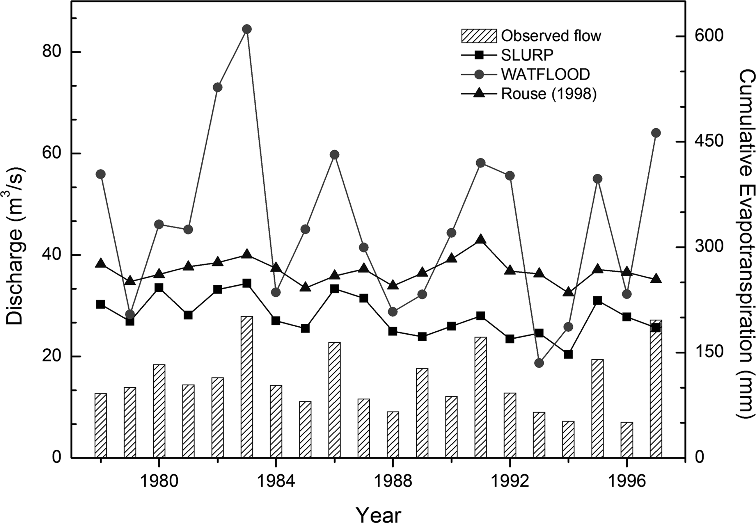
Temporal trends in observed annual hydrograph at the D. River N. Belcher station and cumulative actual evapotranspiration modeled by SLURP, WATFLOOD, and Rouse (1998).

Rainfall-runoff response

Both historical records and model results showed that most light and moderate rainfall events in summer (July–September) were not able to generate notable runoff due to the combined effects from interception, depression and subsurface storage, permafrost, and evapotranspiration. Many lichens, mosses, small shrubs, and conifers flourish in the summer. They have considerable capacities to intercept a great amount of precipitation and this leads to non-negligible water loss for the drainage basin caused by evaporation. Depression storage is mainly referred to the numerous seasonally connected ponds that behave as runoff buffers due to their fluctuating water storage capacities. Highly porous soil and descending frost table allows more water to penetrate into deep soil layers in summer. These distinguished features of subarctic wetlands not only affect snowmelt runoff but also alleviate peak streamflows and extend runoff concentration after rainfall events. Precipitation is retained in soil layers and ponds for a longer period and are more likely to be released as evapotranspiration or groundwater flow rather than surface runoff. As the most significant natural means of cycling water back into the atmosphere, evapotranspiration also tends to be intensified due to higher air temperature and longer daylight period in the summer and, therefore, further reduces surface runoff. These combined factors resulted in the fact that only heavy or continuous rainfall events were able to generate countable runoff.

A high-intensity rainfall event brought large amount of water to the wetland in a short period. After the surface soil layer was saturated, excess water generated flashy runoff, resulting in quicker runoff response. To quantitatively assess the rainfall-runoff response in subarctic wetlands, 44 summer heavy storms (daily amount is more than or equal to 20 mm) that occurred during 1978–1997 were analyzed. Observed streamflow records at the D. River N. Belcher station indicated an average time lag of 3–6 days between the peaks of rainfall and runoff in summer. The modeling results showed that this delay was only 1–3 days, which could be attributed to some unique features of subarctic wetlands (Fig. 5). The variation of permafrost depth, soil water storage capacity, and seasonal pond level can prolong the runoff concentration. Lack of consideration of these buffering effects in both models resulted in those more rapid runoff response. The mean values and standard deviations of rainfall-runoff response in SLURP (1.44 and 0.74 days) and WATFLOOD (1.84 and 0.72 days) indicated that WATFLOOD has relatively longer runoff concentration time, which may be attributed to its depression storage subroutine.

FIG. 5.

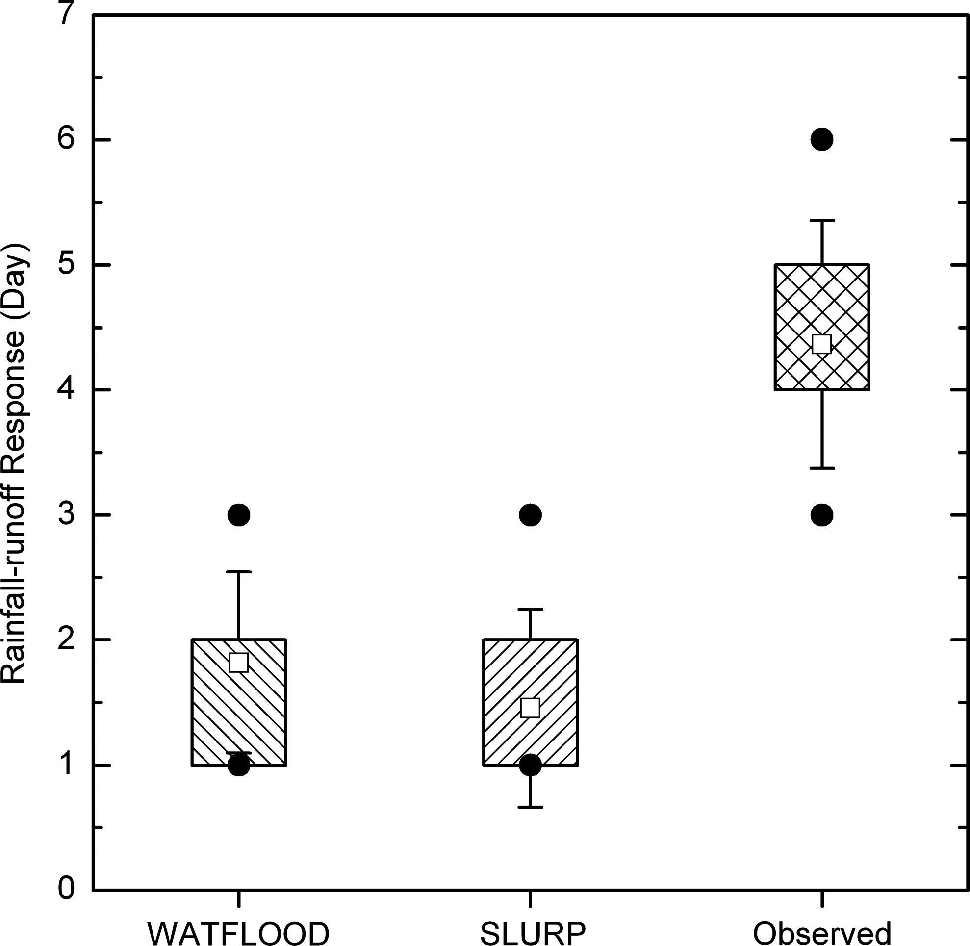
Rainfall-runoff response of high intensity rainfall events in observed records, SLURP, and WATFLOOD at the D. River N. Belcher station (squares show mean values; bottom and top of the boxes describe the 25th and 75th percentiles; circles represent the minimum and maximum values; error bars indicate standard deviations; 36 rainfall events in total from 1978 to 1997 where cumulative daily precipitation exceeds 20 mm).

Conclusions

This research targeted the hydrological processes in subarctic wetlands to understand the water cycle and its unique hydrological features. Based on historical data support and extensive field investigation during 2006–2008 in the Deer River Watershed, Manitoba, two hydrological models, SLURP and WATFLOOD, were applied to simulate wetland hydrology in the typical subarctic region of the HBL. They were further compared from the aspects of delineation approaches, formulations, and parameters, as well as simulation performance, to evaluate their feasibility and effectiveness in modeling subarctic wetlands. Despite the limited applicability to large-scale basins, the HRU watershed delineation approach used in SLURP can recalculate downstream flow values based on transient internal system diversion with good computational efficiency. The GRU approach embedded in WATFLOOD is ideal to couple to remotely sensed data and GIS for large scale basins; however, the heterogeneity may be lost and only land covers differentiation within one grid could be derived. The degree-day snowmelt method is embedded in both models except that SLURP uses a date-varying snowmelt rate that may cause snow depletion to be accelerated. The modeling results indicated that the Morton CRAE method in SLURP had lower evapotranspiration outputs than those from WATFLOOD. Runoff of rain water during summer only occurred after occasional intense precipitation events. It also noted that the lack of considering the existence of permafrost and ponds as well as their interactions in both models appeared to be one of the main reasons for rainfall-runoff modeling inaccuracy. Modifications to both models, such as snowmelt algorithm, permafrost layer, and wetland routing, are recommended for both models to handle these uncertainties and further improve their performance in simulating subarctic wetlands. The findings of this study will be helpful in understanding the hydrologic features of subarctic wetlands and supporting wetland conservation, particularly under climatic change context.

Footnotes

Acknowledgments

Special thanks go to Manitoba Hydro, ArcticNet, NSERC, NFSC, and Churchill Northern Studies Center (CNSC) for funding this work. The advice and help from Dr. Kenneth Snelgrove at Memorial University of Newfoundland and Dr. Tim Papakyriakou at the University of Manitoba are also highly appreciated.

Author Disclosure Statement

The authors declare that no conflicting financial interests exist.

Notation

References

Armstrong

R.N.

, Martz

L.W.

2008. Effects of reduced land cover detail on hydrological model response. Hydrol. Process., 22:2395.

Anderson

E.A.

1973. National Weather Service River Forecast System-Snow Accumulation and Ablation Model. A Technical Report NWS 19 National Oceanographic and Atmospheric Administration (NOAA).

Bongartz

2003. Applying different spatial distribution and modelling concepts in three nested mesoscale catchments of Germany. Phys. Chem. Earth, 28:1343.

Carey

S.K.

, Woo

M.K.

2001. Slope runoff processes and flow generation in a subarctic subalpine catchment. J. Hydrol., 253:110.

Chen

2007. Climate change and pesticide losses in watershed systems: a simulation modeling study. J. Env. Inform., 10:55.

Chen

2008. Health-impact risk assessment for river pollution through a modified contaminant transport model. Water. Air. Soil. Poll., 200:323.

Chen

, Jing

, Snelgrove

, Papakyriakou

2010. Distributed Hydrological Modeling of a Subarctic Wetland System. Procedings of the Canadian Society of Civil Engineering 2010 Annual Conference, Winnipeg, Canada.

Chen

, Li

Y.F.

, Huang

G.H.

, Huang

Y.F.

, Li

Y.R.

2004. PELM: an integrated pesticide losses model for simulating pesticide pollution in a watershed system. J. Environ. Sci. Health. Part. B, B39:613.

Chen

, Li

Y.F.

, Huang

G.H.

, Struger

, Zhang

B.Y.

, Wu

S.M.

2003. Estimation of atrazine loss through the surface runoff from agricultral land in Auglaize-Blanchord watershed, the United States. Water. Quol. Res. J. Can., 38:585.

10.

Dibike

Y.B.

, Coulibaly

2007. Validation of hydrological models for climate scenario simulation: the case of Saguenay watershed in Quebec. Hydrol. Process., 21:3123.

11.

Donald

J.R.

1992. Snowcover depletion curves and satellite snowcover estimates for snowmelt runoff modelling[Ph.D. thesis]University of Waterloo: Waterloo, Canada, 232.

12.

Fassnacht

S.R.

, Soulis

E.D.

, Kouwen

1999. Algorithm application to improve weather radar snowfall estimates for winter hydrologic modelling. Hydrol. Process., 13:3017.

13.

Filoso

, Vallino

, Hopkinson

, Rastetter

, Claessens

2004. Modeling nitrogen transport in the Ipswich river basin, Massachusetts, using a hydrological simulation program in fortran (HSPF) J. Am. Water Resour. Assoc., 40:1365.

14.

Flugel

W.-A.

1995. Delineating hydrological response units by geographical information system analyses for regional hydrological modelling using PRMS/MMS in the drainage basin of the river Bröl, Germany. Hydrol. Process., 9:423.

15.

Granger

R.J.

1995. A feedback approach for the estimation of evapotranspiration using remotely sensed data. Kite

G.W.

, Pietroniro

, Pultz

Applications of Remote Sensing in Hydrology. Proceedings of the Second International Workshop, 18–20 October, 1994. NHRI: Saskatoon, 211–222.

16.

Greene

R.G.

, Cruise

J.F.

1995. Urban watershed modeling using geographic information system. J. Water Resour. Plann. Manage. ASCE, 121:318.

17.

Haberlandt

, Kite

G.W.

1998. Estimation of daily space-time precipitation series for macroscale hydrological modelling. Hydrol. Process., 12:1419.

18.

Hamlin

L.P.B.

1996. Snowmelt hydrologic modelling of northern wetland dominated river basins[M.A.Sc. thesis]University of Waterloo: Waterloo, Canada, 213.

19.

Hargraeves

G.H.

, Samani

Z.A.

1982. Estimating potential evapotranspiration. ASCE J. Irrig. Drain. Div., 108:225.

20.

Hattermann

F.F.

, Krysanova

, Hesse

2008. Modelling wetland processes in regional applications. Hydrol. Sci. J., 53:1001.

21.

Jing

2009. Hydrological monitoring and modelling of the Deer River watershed with SLURP and WATFLOOD[M.Eng. thesis]Memorial University of Newfoundland: St. John's, Canada.

22.

Jing

, Chen

2011. Field investigation and hydrological modelling of a subarctic wetland—the Deer River watershed. J. Env. Inform., 17:36.

23.

Jing

, Chen

, Snelgrove

, Papakyriakou

2009. Hydrological monitoring and characterization of a subarctic wetland in the Hudson Bay lowlands. Proceedings of the Canadian Society of Civil Engineering 2009 Annual ConferenceGC-135-1-10, St. John'sCanada.

24.

Jing

, Chen

, Zhang

B.Y.

2010. A comparison study on distributed hydrological modelling of a subarctic wetland system. Procedia Environmental Science, 2:1043.

25.

Kite

G.W.

1997. Manual for the SLURP Hydrological Model V.11. National Hydrology Research Institute: Saskatoon, Canada.

26.

Kite

G.W.

2002. Manual for the SLURP hydrological model, v12.2. International Water Management Institute: Colombo, Sri Lanka.

27.

Kite

G.W.

, Dalton

, Dion

1994. Simulation of streamflow in a macroscale watershed using general circulation model data. Water Resour. Res., 30:1547.

28.

Kouwen

2008. Manual for WATFLOOD/WATROUTE—Hydrological Model Routing & Flow Forecasting System. University of Waterloo: Waterloo, Canada.

29.

Kouwen

, Soulis

E.D.

, Pietroniro

, Donald

, Harrington

R.A.

1993. Grouped response units for distributed hydrologic modeling. J. Water. Res. ASCE, 119:289.

30.

Kustas

W.P.

, Rango

, Uijlenhoet

1994. A simple energy budget algorithm for the snowmelt runoff model. Water. Resour. Res., 30:1515.

31.

Leon

L.F.

, Soulis

E.D.

, Kouwen

, Farquhar

G.J.

2001. Nonpoint source pollution: a distributed water quality modeling approach. Water Res., 35:997.

32.

, Chen

, Husain

2011. IRFAM: Integrated rule-based fuzzy adaptive resonance theory mapping system for watershed modeling. J. Hydrologic. Engrg., 16:21.

33.

Linsley

R.K.

, Kohler

M.A.

, Paulhus

J.L.H.

1949. Applied Hydrology. New York: McGraw-Hill.

34.

Mansell

R.S.

, Bloom

S.A.

, Sun

2000. A Model for wetland hydrology: description and validation. Soil. Sci., 165:384.

35.

Metcalfe

R.A.

, Buttle

J.M.

2001. Soil partitioning and surface store controls on spring runoff from a boreal forest peatland basin in north-central Manitoba, Canada. Hydrol. Process., 15:2305.

36.

Mills

G.F.

, Veldhuis

, Forrester

D.B.

, Schmidt

1976. A guide to bio-physical land classification in Manitoba. Northern Resource Information ProgramDepartment of Renewable Resources and Transportation Services and Canada-Manitoba Soil Survey.

37.

Mohan

1991. Intercomparison of evapotranspiration estimates. Hydrol. Sci. J., 36:447.

38.

Morton

F.I.

1983. Operational estimates of areal evapotranspiration and their significance to the science and practice of hydrology. J. Hydrol., 66:77.

39.

Penman

H.L.

1948. Natural evaporation from open water, bare soil and grass. Proc. Roy Soc. Lond. A, 193:120.

40.

Philip

J.R.

1954. An infiltration equation with physical significance. Soil Sci., 77:153.

41.

Pietroniro

, Leconte

, Toth

, Peters

D.L.

, Kouwen

, Conly

F.M.

, Prowse

2006. Modelling climate change impacts in the Peace and Athabasca catchment and delta: III-integrated model assessment. Hydrol. Process., 20:4231.

42.

Pohl

, Davison

, Marsh

, Pietroniro

2005. Modelling spatially distributed snowmelt and meltwater runoff in a small arctic catchment with a hydrology-land surface scheme (WATCLASS) Atmos. Ocean, 43:193.

43.

Priestly

C.H.B.

, Taylor

R.J.

1972. On the assessment of surface heat flux and evaporation using large-scale parameters. Mon. Weather Rev., 100:81.

44.

Price

J.S.

, Branfireun

B.A.

, Waddington

J.M.

, Devito

K.J.

2005. Advances in Canadian wetland hydrology, 1999–2003. Hydrol. Process., 19:201.

45.

Rango

, Martinec

1995. Revisiting the degree-day method for snowmelt computations. Water. Resour. Bull. AWRA., 31:657.

46.

Rouse

W.R.

1998. A water balance model for a subarctic sedge fen and its application to climate change. Clim. Change, 38:207.

47.

Rouse

W.R.

, Douglas

M.S.V.

, Hecky

, Hershey

A.E.

, Kling

G.W.

, Lesack

, Marsh

, Mcdonald

, Nicholson

B.J.

, Roulet

N.T.

, Smol

J.P.

1997. Effects of climate change on the fresh waters of arctic and subarctic northern America. Hydrol. Process., 11:873.

48.

Schmalz

, Tavares

, Fohrer

2008. Modelling hydrological processes in mesoscale lowland river basins with SWAT-capabilities and challenges. Hydrol. Sci. J., 53:989.

49.

See

R.B.

, Naftz

D.L.

, Qualls

C.L.

1992. GIS-assisted regression analysis to identify sources of selenium in streams. Water. Resour. Bull., 28:315.

50.

Seglenieks

F.R.

1994. Application of remote sensing and ground measurements to calibrate the hydrologic model WATFLOOD[M.A.Sc. thesis]University of Waterloo: Waterloo, Canada, 162.

51.

Shaffer

P.W.

, Kentula

M.E.

, Gwin

S.E.

1999. Characterization of wetland hydrology using hydrogeomorphic classification. Wetlands, 19:490.

52.

Shaw

D.A.

, Martz

L.W.

, Pietroniro

2005. A methodology for preserving channel flow networks and connectivity patterns in large-scale distributed hydrological models. Hydrol. Process., 19:149.

53.

Shin

H.J.

, Kim

S.J.

2007. Assessment of climate change impact on snowmelt in the two mountainous watersheds using CCCma CGCM2. KSCE J. Civil Eng., 11:311.

54.

Spittlehouse

D.L.

1989. Estimating evapotranspiration from land surfaces in British Columbia. Black

T.A.

et al. Estimation of Areal Evapotranspiration. IAHS Publication No. 177, 245–253. United Kingdom.

55.

SPOT IMAGE and VITO. 2008. Welcome to the image processing and archiving centre. Belgium: VITO www.vgt.vito.be

56.

St Laurent

M.E.

, Valeo

2007. Large-scale distributed watershed modelling for reservoir operations in cold boreal regions. Can. J. Civil. Eng., 34:525.

57.

Stadnyk

2008. Mesoscale hydrological model validation and verification using stable water isotopes: The isoWATFLOOD[PhD. thesis]University of Waterloo: Waterloo, Canada.

58.

Stow

D.A.

, Hope

, McGuire

, Verbyla

, Gamon

, Huemmrich

, Houston

, Racine

, Sturm

, Tape

, Hinzman

, Yoshikawa

, Tweedie

, Noyle

, Silapaswan

, Douglas

, Griffith

, Jia

, Epstein

, Walker

, Daeschner

, Petersen

, Zhou

L.M.

, Myneni

2004. Remote sensing of vegetation and land-cover change in Arctic Tundra Ecosystems. Remote Sens. Environ., 89:281.

59.

Ström

, Christensen

T.R.

2007. Below ground carbon turnover and greenhouse gas exchanges in a subarctic wetland. Soil. Biol. Biochem., 39:1689.

60.

, Stolte

W.J.

, Van der Kamp

2000. Modelling Canadian prairie wetland hydrology using a semi-distributed streamflow model. Hydrol. Process., 14:2405.

61.

Thompson

J.R.

, Sørenson

H.R.

, Gavin

, Refsgaard

2004. Application of the coupled MIKE SHE/MIKE 11 modelling system to a lowland wet grassland in southeast England. J. Hydrol., 293:151.

62.

Thorne

2004. Simulating streamflow of a large mountainous catchment using different sets of climatic data[M.Sc. thesis]McMaster University: Hamilton, Canada.

63.

USGS. 2008. The National Map Seamless Server. USGS: science for a changing world. http://seamless.usgs.gov/index.php

64.

Van der Linden

, Woo

M.K.

2003. Application of hydrological models with increasing complexity to subarctic catchments. J. Hydrol., 270:145.

65.

Wessel

D.A.

, Rouse

W.R.

1994. Modelling evaporation from Wetland Tundra. Bound-Lay. Meteorol., 68:109.

66.

Woo

M.K.

, Marsh

, Pomeroy

J.W.

2000. Snow, frozen soils and permafrost hydrology in Canada, 1995–1998. Hydrol. Process., 14:1591.

67.

Woo

M.K.

, Young

2003. Hydrogeomorphology of patchy wetlands in the high arctic, polar desert environment. Wetlands, 23:291.

68.

Woo

M.K.

, Thorne

2006. Snowmelt contribution to discharge from a large mountainous catchment in subarctic Canada. Hydrol. Process., 20:2129.

69.

K.S.

, Johnston

C.A.

2007. Hydrologic comparison between a forested and a wetland/lake dominated watershed using SWAT. Hydrol. Process., 22:1431.