Water Quality Modeling in a Tidal Estuarine System Using a Three-Dimensional Model

Abstract

A three-dimensional water quality model has been developed and applied to the Danshuei River estuarine system and adjacent coastal sea. The model considered various species of nitrogen, phosphorus, and silicon, organic carbon, phytoplankton, and zooplankton as well as dissolved oxygen and was driven by a three-dimensional hydrodynamic model. The hydrodynamic and water quality model was validated with observational tidal range, water surface elevation, velocity, salinity, and water quality state variables. According to the analyses of statistical error, predictions of hydrodynamic, salinity, dissolved oxygen, and nutrients from the model simulation quantitatively agreed with the observed data. Based on the validated model, model sensitivity analyses were conducted with sediment oxygen demand (SOD), benthic flux of ammonium nitrogen, and freshwater discharge at upstream boundaries. If SOD value increased 50%, the maximum rates for decreasing dissolved oxygen were 47.9% and 94.2% at the surface and bottom layers, respectively, in the Danshuei River-Tahan Stream. Model results showed that SOD had a significant impact on the distribution of dissolved oxygen concentration along the river. Low freshwater discharges at upstream boundaries resulted in lower dissolved oxygen concentration and higher nutrients in the Danshuei River estuarine system.

Introduction

Estuaries receive organic matter and inorganic nutrients from the land and represent important systems where terrestrial nutrients and organic matter are subject to physical and biogeochemical processes before entering the coastal ocean. As a result, the water quality, ecology, and biodiversity of estuarine waters are under the threat of increasing anthropogenic nutrient inputs. Adverse impacts on the estuarine ecosystem by human activities have been widely reported; studies and management of the estuarine environments have gained more and more attention in recent decades (Wool et al., 2003; Zheng et al., 2004; McGlathery et al., 2007; Brush and Nixon, 2010).

Water quality models are essential tools for the assessment of the impact of estuarine ecosystem changes in response to nutrient inputs as well as the interactions occurring in the system. The models become important tools for effective management of estuarine system and for the design and optimization of discharge regimes. The models may be used to set up surveillance procedures and assist the decision-making process; therefore, environmental objectives can be met and adequate safety margins can be defined at a realistic coast. Estuarine water quality models are necessary to describe the problem of allowing discharges, which are variable by nature and monitoring assessment.

The proper simulation of water quality characteristics in an estuarine system principally depends on two factors. First, a good representation of the hydrodynamic field is essential because it provides the basic physical transport information for each water quality variable. Second, biogeochemical processes are usually represented by various forms of empirical formulations in the model, so extensive data analysis is needed to provide values to the unique parameters in equations (Cerco and Cole, 1993).

Numerical water quality models have been widely used to study and manage water quality conditions in aquatic systems. Deterministic models for the water quality conditions are based on mass balance equations for dissolved and particulate substances in water column, which consist of physical transport (advective and turbulent diffusive transport) processes and biogeochemical processes. Information on physical processes is usually obtained by applying hydrodynamic models. Traditionally, vertical (laterally averaged) and horizontal two-dimensional models have not well represented the spatial variations, unlike the three-dimensional model, in estuarine systems, such as the model applied in the Danshuei River estuary, Taiwan (Liu et al., 2005), the Patuxent Estuary, United States (Lung and Nice, 2007), and the Urdaibai Estuary, Spain (Garcia et al., 2010). This is the reason that the three-dimensional numerical model has been considered to be adopted in the present study.

Recently, three-dimensional hydrodynamic and water quality (eutrophication) models have been widely applied to estuarine and oceanographic studies (Wool et al., 2003; Chau, 2005; Park et al., 2005; Lessin and Raudsepp, 2006; Lin et al., 2007). For example, Zheng et al. (2004) coupled a three-dimensional physical and water quality model to study the Satilla River Estuary, Georgia. The physical model is the modified ECOM-Si version with inclusion of flooding/draining process. The water quality model is a modified WASP5 with inclusion of nutrient fluxes from the bottom sediment layer. Lin et al. (2008) applied a coupled hydrodynamic and water quality model based on the three-dimensional hydrodynamic-eutrophication model to examine the estuarine system responses to high river discharge events and nutrient loading variation from the drainage basin in the Cape Fear River Estuary. Timmermann et al. (2010) developed a coupled three-dimensional hydrodynamic-ecological model with numerical nitrogen tracking for Horsens Estuary, Demark, to investigate the impact of stream nitrogen reductions on nitrate and chlorophyll a concentrations.

A huge amount of domestic wastewater, mostly untreated raw sewage, was discharged into the estuary daily. The water quality of the estuary has been severely degraded for decades. Hypoxic/anoxic conditions commonly occur in the upper and middle reaches of the estuary during summer months (Liu et al., 2001b). Because of the complexity of the transport and huge pollutant loadings with the Danshuei River estuarine system, a coupled three-dimensional hydrodynamic Eulerian-Lagrangian circulation model (ELCIRC-3D model) and water quality model was developed and applied to investigate the water quality conditions in the estuarine system. The model was validated with observational tidal range, water surface elevation, current velocity, salinity, and water quality state variables. Model sensitivity analysis was then conducted to comprehend the parameters that affect the dissolved oxygen and nutrient distributions along the river. The water quality modeling results with low freshwater discharge at upstream boundaries were also compared with the median freshwater discharge.

Description of Study Area and Background

The Danshuei River, located on the outskirts of Taipei, constitutes the largest estuary in Taiwan. It consists of three major tributaries: the Tahan Stream, Hsintien Stream, and Keelung River (Fig. 1). The Tahan Stream joins the Hsintien Stream at Wan-Hwa. The river then combines with the Keelung River at Kuan-Du. The segment of the estuary from Wan-Hwa to the estuary's mouth is called the main Danshuei River. In addition to the mainstream of the Danshuei River, the lower reaches of the three major tributaries are also influenced by tide. Seawater intrusion reaches into all three tributaries except during periods of very high river inflows. The hydrodynamic characteristics in the system are mainly controlled by tide, river inflow, and the density gradient induced by the mixing of saline and freshwater (Hsu et al., 1999; Liu et al., 2001a, 2007). Because of the relatively large tidal range compared with the depth of the system, the residence time of the main stream estuary was found to be 2.2 days or less (Wang et al., 2004).

FIG. 1.

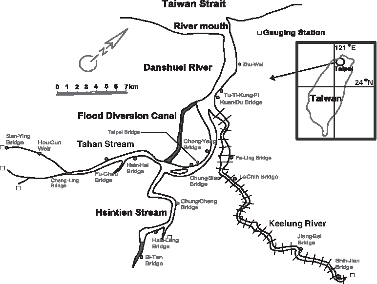
Map of Danshuei River estuarine system.

The estuarine portion of the river system runs through the capital city of Taipei, with a population of about 6 millions in its metropolitan area. A huge amount of pollutant loadings was discharged into the river system and resulted in low dissolved oxygen and high nutrients. Viable biological activities are observed only in the lowest reach of the estuary where the pollutant concentrations are reduced as a result of dilution by sea water. The research group from the Academia Sinica of Taiwan conducted a 3-year observational study of the system from 1998 to 2001. They reported that the chlorophyll a concentration hardly exceeded 5 mg/m³. The primary production rate was reported to be on the order of 0.2 g C/m³/day. The zooplankton biomass was observed to range from 1 to 14 mg C/m³. Hsieh et al. (2010) examined how tidal changes and which physical factors affected holo- and meroplankton assemblages in the Dasnhuei River estuary. They found that during tidal flooding, the water mass properties changed to low salinity (5–16 ppt) and high particulate organic carbon (2.6–4.5 mg/L).

Numerical Model

Hydrodynamic model

ELCIRC is a model designed for the effective three-dimensional simulation of both barotropic and baroclinic processes across river-to-ocean scales (Zhang et al., 2004). The shallow water equations are solved by using a finite-volume/finite-difference semi-implicit Eulerian-Lagrangian algorithm to enhance computational efficiency and assure volume conservation. The employment of horizontally unstructured grids allows for a better fit of the shoreline and for greater freedom in varying the grid size without the trade-off with computer time or resolution.

The free surface elevation, water velocities, and salinity are computed using a set of six equations with hydrostatic assumption based on the Boussinesq approximation as follows: \documentclass{aastex} \usepackage{amsbsy} \usepackage{amsfonts} \usepackage{amssymb} \usepackage{bm} \usepackage{mathrsfs} \usepackage{pifont} \usepackage{stmaryrd} \usepackage{textcomp} \usepackage{portland, xspace} \usepackage{amsmath, amsxtra} \pagestyle{empty} \DeclareMathSizes {10} {9} {7} {6} \begin{document} \begin{align*} \frac {\partial u} {\partial x} + \frac {\partial v} {\partial y} + \frac {\partial w} {\partial z} = 0 \tag {1} \end{align*} \end{document} \documentclass{aastex} \usepackage{amsbsy} \usepackage{amsfonts} \usepackage{amssymb} \usepackage{bm} \usepackage{mathrsfs} \usepackage{pifont} \usepackage{stmaryrd} \usepackage{textcomp} \usepackage{portland, xspace} \usepackage{amsmath, amsxtra} \pagestyle{empty} \DeclareMathSizes {10} {9} {7} {6} \begin{document} \begin{align*} \frac {\partial \eta} {\partial t} + \frac {\partial} {\partial x} \int_ {H_ {\rm R} - h} ^ {H_ {\rm R} + \eta} udz + \frac {\partial} {\partial y} \int_ {H_ {\rm R} - h} ^ {H_ {\rm R} + \eta} vdz = 0 \tag {2} \end{align*} \end{document} \documentclass{aastex} \usepackage{amsbsy} \usepackage{amsfonts} \usepackage{amssymb} \usepackage{bm} \usepackage{mathrsfs} \usepackage{pifont} \usepackage{stmaryrd} \usepackage{textcomp} \usepackage{portland, xspace} \usepackage{amsmath, amsxtra} \pagestyle{empty} \DeclareMathSizes {10} {9} {7} {6} \begin{document} \begin{align*} \frac {\partial u} {\partial t} + u \frac {\partial u} {\partial x} + v \frac {\partial u} {\partial y} + w \frac {\partial u} {\partial z} = fv - \frac {\partial} {\partial x} \left\{g (\eta - \alpha \varphi) + \frac {P_ {\rm a}} {\rho_ {\rm o}} \right\} - \frac {g} {\rho_o} \int_z^ {H_ {\rm R} + \eta} \frac {\partial p} {\partial x} dz + \frac {\partial} {\partial z} \left(K_ {\rm mv} \frac {\partial u} {\partial z} \right) + F_ {\rm mx} \tag {3} \end{align*} \end{document} \documentclass{aastex} \usepackage{amsbsy} \usepackage{amsfonts} \usepackage{amssymb} \usepackage{bm} \usepackage{mathrsfs} \usepackage{pifont} \usepackage{stmaryrd} \usepackage{textcomp} \usepackage{portland, xspace} \usepackage{amsmath, amsxtra} \pagestyle{empty} \DeclareMathSizes {10} {9} {7} {6} \begin{document} \begin{align*} \frac {\partial v} {\partial t} + u \frac {\partial v} {\partial x} + v \frac {\partial v} {\partial y} + w \frac {\partial v} {\partial z} = - fu - \frac {\partial} {\partial y} \left\{g (\eta - \alpha \varphi) + \frac {P_ {\rm a}} {\rho_ {\rm o}} \right\} - \frac {g} {\rho_o} \int_z^ {H_ {\rm R} + \eta} \frac {\partial p} {\partial y} dz + \frac {\partial} {\partial z} \left(K_ {\rm mv} \frac {\partial v} {\partial z} \right) + F_ {\rm my} \tag {4} \end{align*} \end{document} \documentclass{aastex} \usepackage{amsbsy} \usepackage{amsfonts} \usepackage{amssymb} \usepackage{bm} \usepackage{mathrsfs} \usepackage{pifont} \usepackage{stmaryrd} \usepackage{textcomp} \usepackage{portland, xspace} \usepackage{amsmath, amsxtra} \pagestyle{empty} \DeclareMathSizes {10} {9} {7} {6} \begin{document} \begin{align*} \frac {\partial S} {\partial t} + \frac {\partial (uS)} {\partial x} + \frac {\partial (vS)} {\partial y} + \frac {\partial (wS)} {\partial z} = \frac {\partial} {\partial z} \left(K_ {\rm sv} \frac {\partial S} {\partial z} \right) + F_ {\rm s} \tag {5} \end{align*} \end{document} \documentclass{aastex} \usepackage{amsbsy} \usepackage{amsfonts} \usepackage{amssymb} \usepackage{bm} \usepackage{mathrsfs} \usepackage{pifont} \usepackage{stmaryrd} \usepackage{textcomp} \usepackage{portland, xspace} \usepackage{amsmath, amsxtra} \pagestyle{empty} \DeclareMathSizes {10} {9} {7} {6} \begin{document} \begin{align*} \rho = \rho_{\rm o} (p , S) \tag{6} \end{align*} \end{document}

where (x, y) are the horizontal Cartesian coordinates; (φ, λ) are the latitude and longitude; z is the vertical coordinate, positive upward; t is time; H_R is the z-coordinate at the reference level (mean sea level); η (x, y, t) is the free-surface elevation; h(x, y) is the bathymetric depth; u, v, and w are the velocities in x, y, and z directions, respectively; fis the Coriolis force; g is the acceleration of gravity; p is pressure; φ(φ, λ) is the tidal potential; α is the effective Earth elasticity factor (≈0.69; Foreman et al., 1993); \documentclass{aastex} \usepackage{amsbsy} \usepackage{amsfonts} \usepackage{amssymb} \usepackage{bm} \usepackage{mathrsfs} \usepackage{pifont} \usepackage{stmaryrd} \usepackage{textcomp} \usepackage{portland, xspace} \usepackage{amsmath, amsxtra} \pagestyle{empty} \DeclareMathSizes {10} {9} {7} {6} \begin{document} $$\rho ({\vec x} , t)$$ \end{document} is the water density; P_a(x, y, t) is atmospheric pressure at the free surface; S is salinity; K_mv is the vertical eddy viscosity; K_sv is the vertical eddy diffusivity for salinity; F_mx and F_my are the horizontal diffusion for momentum equation in x and y directions, respectively; and F_s is the horizontal diffusion for transport equation. By default, the reference value ρ_o is set to 1,025 kg/m³.

The numerical algorithm of ELCIRC used a semi-implicit scheme. The barotropic pressure gradient in the momentum equation and the flux term in continuity are treated semi-implicitly, with implicitness factor 0.5 ≤ θ ≤ 1. According to Casulli and Walters (2000), this ensures both stability and computational efficiency.

The detailed description of vertical boundary conditions for primary equation including horizontal momentum at surface boundary and bottom boundary as well as parameterization of turbulent vertical mixing can be found in the study by Zhang et al. (2004).

Water quality model

To meet the essential requirement of mass conservation for a water quality model, the finite volume/finite difference upwind-based scheme used by the water quality model CE-QUAL-ICM (a multi-dimensional water quality model for surface water; Cerco and Cole, 1995) has been adopted and modified. Following the CE-QUAL-ICM formulation, the mass balance equation for each water quality state variable can be written as \documentclass{aastex} \usepackage{amsbsy} \usepackage{amsfonts} \usepackage{amssymb} \usepackage{bm} \usepackage{mathrsfs} \usepackage{pifont} \usepackage{stmaryrd} \usepackage{textcomp} \usepackage{portland, xspace} \usepackage{amsmath, amsxtra} \pagestyle{empty} \DeclareMathSizes {10} {9} {7} {6} \begin{document} \begin{align*} \frac {\partial C} {\partial t} + \frac {\partial (uC)} {\partial x} + \frac {\partial (vC)} {\partial y} + \frac {\partial (wC)} {\partial z} = \frac {\partial} {\partial z} \left(K_ {\rm sv} \frac {\partial C} {\partial z} \right) + F_ {\rm c} + S_ {\rm c} \tag {7} \end{align*} \end{document}

where C is the concentration of a water quality state variable; F_c is the horizontal diffusion for transport equation; and S_c is the internal and external sources and sinks per unit volume.

The biogeochemical processes simulated in the developed model include nutrient dynamics, primary production and plankton dynamics, and dissolved oxygen budgeting. A total of 22 state variables (Table 1) were simulated by the model. Figure 2 is a schematic diagram that shows the interrelationship among the state variables. Each solid-line rectangle represents a state variable for which the concentration in the water column has to be computed. The variables enclosed by dash-line rectangles are not explicitly modeled; however, their contributions to the modeled system are implicitly accounted for with simple equations. An arrow between any two state variables represents the biogeochemical processes transforming one state variable into the other. The arrows with one end not attaching to any state variable represent processes that transform, or transfer, a state variable out of (or into) the modeled system. Each arrow is represented by at least one mathematical equation in the model.

FIG. 2.

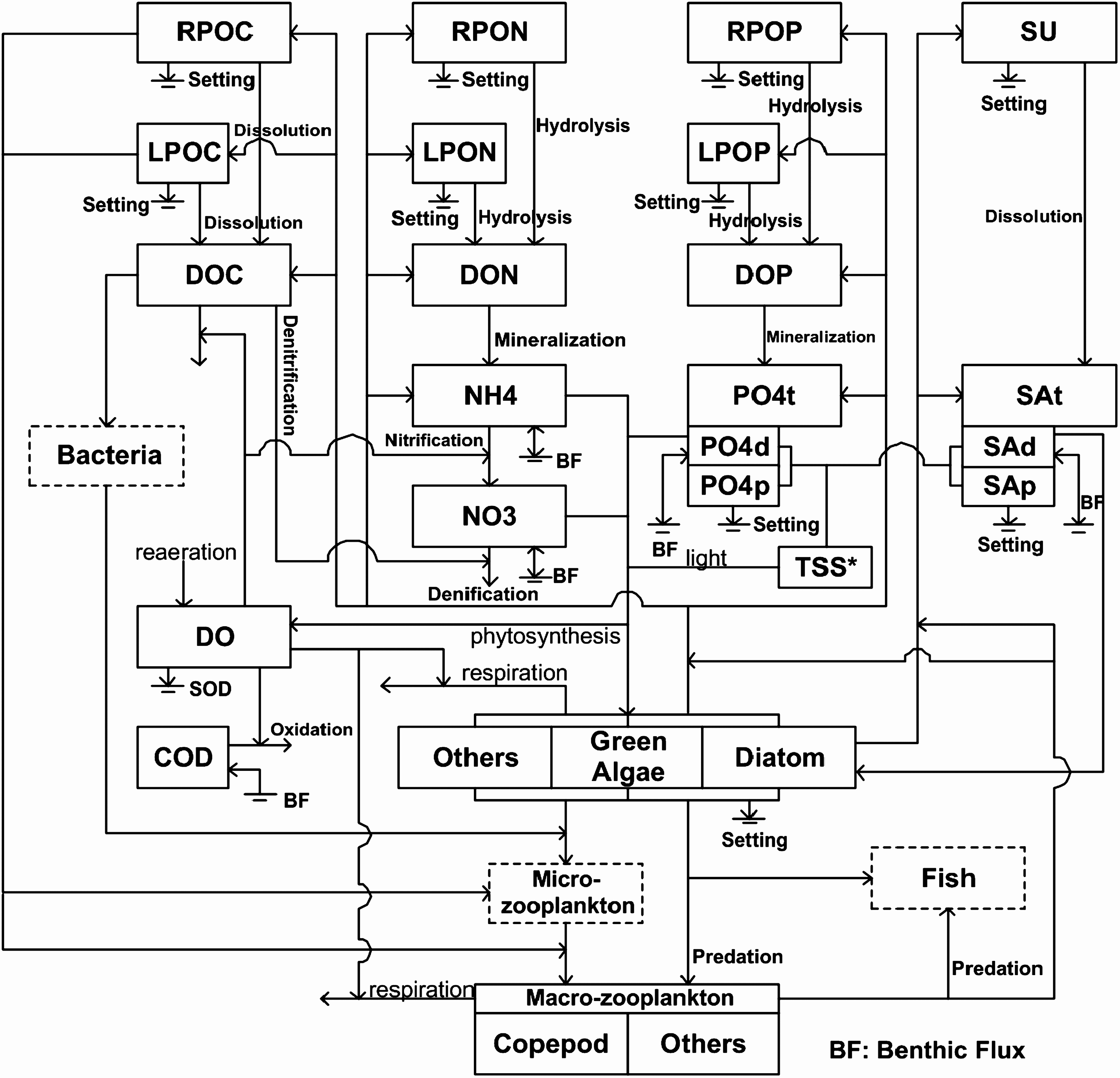
Schematic diagram showing interrelationships of the state variables in water quality model.

Table 1.

List of State Variables Used in Water Quality Model

Variable	Full name
RPOC	Refractory particulate organic carbon
LPOC	Labile particulate organic carbon
DOC	Dissolved organic carbon
DO	Dissolved oxygen
COD	Chemical oxygen demand
RPON	Refractory particulate organic nitrogen
LPON	Labile particulate organic nitrogen
DON	Dissolved organic nitrogen
NH4	Ammonium nitrogen
NO3	Nitrite plus nitrate nitrogen
RPOP	Refractory particulate organic phosphorus
LPOP	Labile particulate organic phosphorus
DOP	Dissolved organic phosphorus
PO4t	Total phosphate including dissolved and particulate phosphate
SU	Particulate biogenic silicate
SAt	Available silicate including dissolved and particulate available silicate
TSS	Total suspended solid
PB₁	Diatoms
PB₂	Green algae
PB₃	Other phytoplankton
ZB₁	Copepods
ZB₂	Other zooplankton

The overall structure of the modeling system is adopted from the Chesapeake Bay Program's water quality model, CE-QUAL-ICM (Cerco and Cole, 1995), and modified based on the past research of the Danshuei River estuary (Wang, 2005).

For the transport equation, equation (7) is discretized and solved in two steps. First, an intermediate value is computed, which includes the effects of change in cell volume, horizontal advection and diffusion, and external loads and kinetic sources and sinks. Second, the effects of vertical advection and diffusion are computed. Horizontal advection and diffusion terms are discretized explicitly, whereas the vertical advection and diffusion term are treated with a semi-implicit approach.

Model implementation

In the present study, the bottom topography data in the coastal sea and Danshuei River estuarine system were obtained from the National Center for Ocean Research and Water Resources Agency, Taiwan. The modeling domain in horizontal plane covers 55 km × 50 km. The greatest depth in the study area is 110 m (below mean sea level) near the northeast corner of the model in the coastal sea. As ELCIRC uses a combination of Eulerian-Lagrangian and implicit time stepping, it does not have to satisfy the usual Courant-Friedrich-Levy constraint for numerical stability. Applying this baroclinic criterion to our model grid spacing and salinity values, Δt was chosen to be 300 s. Trial and error tests with other time steps demonstrated that the model results did not improve significantly with lower values. The model mesh for the Danshuei River estuarine system and its adjacent coastal sea consisted of 6,969 polygons and 4,098 grids (Fig. 3). To save computational time, higher resolution grids were used in the Danshuei River estuary and coarser grids in the coastal sea. Because the model domain includes deep bathymetry in the coastal ocean and a shallow area in the channel, 32 levels varying in thickness from 1 to 10 m were adopted for vertical discretization in ELCIRC.

FIG. 3.

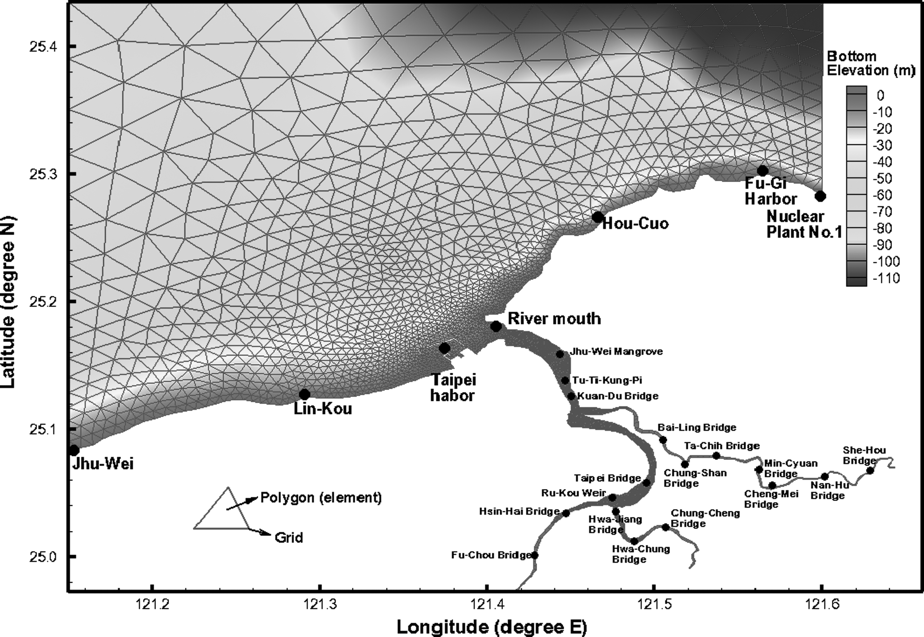
Unstructured grids generation in modeling domain.

Model Validation

Tidal range

The model was calibrated with the observed astronomical tides in the Danshuei River estuarine system and along the northern coastline. The model calibration was carried out with upstream boundary conditions at the three tidal limits having the constant discharges of the long-term means. The freshwater discharges at upstream boundary conditions were specified with 12.8, 23.7, and 9.83 m³/s in the Tahan Stream, Hsintien Stream, and Keelung River, respectively. A five-constituent tide (i.e., M₂, S₂, N₂, K₁, and O₁) was used for the boundary conditions along the three open boundaries. The amplitudes and phases of the tidal constituents at the two land points on the open boundary were derived from the tide records at the respective locations, Jhu-Wei and Nuclear Power Plant No. 1. The amplitudes and phases at the two offshore corner points were referred from the work by Liu et al. (2007). Linear interpolation was employed for locations along the boundary between any two corner points. Table 2 lists the amplitudes and phases used for the model simulation at the coastal sea boundaries.

Table 2.

Amplitudes and Phases Used for Model Simulation at the Coastal Sea Boundaries

	East boundary		Northeast boundary		West boundary		Northwest boundary
Constituent	Amplitude	Phase	Amplitude	Phase	Amplitude	Phase	Amplitude	Phase
(period)	(m)	(degree)	(m)	(degree)	(m)	(degree)	(m)	(degree)
M ₂	0.47	172.37	0.6711	171.33	0.1236	181.63	1.3716	180.42
S ₂	0.12	331.75	0.1866	332.25	0.3452	354.5	0.3987	355.2
N ₂	0.10	262.74	0.1370	262.35	0.2252	281.373	0.2526	279.41
K ₁	0.21	232.33	0.2223	234.2	0.2121	246.06	0.2275	246.69
O ₁	0.17	67.54	0.170	67.05	0.1748	75.02	0.1866	74.40

The model calibration proceeded by adjusting the values of model roughness height until reasonable agreement was achieved between the computed tidal ranges and the average values derived from observation data at all available tide stations. The model was simulated for 20 days, but the modeling results at the last 5 days were taken as an average to calculate tidal range. Figure 4 presents the comparisons between model results and field observations along the river channels. The slightly landward decrease of the tidal range near the Danshuei River mouth may be the result of high frictional energy loss in that reach of the river. At the uppermost reaches of all three branches, the tidal range decrease sharply as the result of the rapid rise in the river bottom. Finally, the tidal range reaches its limit when the river bottom rises above high tide level. However, the model overestimates the tidal range at Tu-Ti-Kung-Pi, whereas it underestimates the tidal range at Chung-Cheng Bridge. Table 3 presents the comparisons between computed results and field observations along the coastline. The results show that the computed tidal ranges faithfully agree with the observation data along the coastline. Finally, the constant bottom roughness height (z_o = 0.005 m) is adopted in the model through model calibration.

FIG. 4.

Comparison between the observed and simulated mean tidal ranges in Danshuei River estuarine system. D, Danshuei River; H, Hsintien Stream; K, Keelung River.

Table 3.

Comparison Between the Observed and Computed Mean Tidal Ranges Along the Coastline

	Mean tidal range (m)
Station	Observation	Computation
Fu-Gi harbor	1.42	1.43
Hou-Cuo	1.83	1.87
River mouth	2.16	2.17
Lin-Kou	2.37	2.31

Tidal elevation

The model validation was conducted with daily freshwater discharges at upstream boundaries in the Tahan Stream, Hsintien Stream, and Keelung River in 2002. The model was run for a 1-year simulation. Before the 1-year simulated run, the model was spun up 15 days to reach an equilibrium state. These conditions served to investigate the model response to the interactions of tidal forcing and varying river discharge. The freshwater discharge inputs from three tributaries (i.e., Tahan Stream, Hsintien Stream, and Keelung River) are presented in Fig. 5a. Figure 5b–g presents the computed surface elevations and the measured data at six stations (Danshuei River mouth, Tu-Ti-Kung-Pi, Taipei Bridge, Hsin-Hai Bridge, Chung-Cheng Bridge, and Ta-Chih Bridge). It shows that upriver stations (Fig. 5e, f) have a more conspicuous response to the pulse of high freshwater discharge than downstream stations. In general, the modeling results accurately reproduced the water level variations. The mean absolute errors of the difference between the measured hourly surface elevations and the computed surface elevations during July 1–11, 2002, at the Danshuei River mouth, Tu-Ti-Kung-Pi, Taipei Bridge, Hsin-Hai Bridge, Chung-Cheng Bridge, and Ta-Chih Bridge were 0.33, 0.26, 0.39, 0.31, 0.37, and 0.37 m, respectively. The corresponding root-mean-square errors were 0.39, 0.33, 0.49, 0.41, 0.47, and 0.45 m, respectively.

FIG. 5.

(a) Freshwater discharge inputs from three tributaries from July 1–11, 2002, and a comparison of water surface elevations at the following locations: (b) the Danshuei River mouth, (c) the Tu-Ti-Kung-Pi, (d) the Taipei Bridge, (e) the Hsin-Hai Bridge, (f) Chung-Cheng Bridge, and (g) the Ta-Chih Bridge.

Tidal current

To evaluate the model's ability in the estuary, an intensive survey of the current was conducted at five transects on April 26, 2002. The current was measured by trained technicians on boats every half hour for a period of 13 daylight hours. The velocity data were obtained using handheld Price current meters that measured the magnitude of current but not its direction. The data were recorded by hand, and flow was visually determined in either the “ebb” or “flood” direction. We encountered some uncertainty in determining the direction of current during slack tides. To compare the measured and computed velocities, the computed velocity in the horizontal plane was converted to the velocity along the channel. Figure 6a–e compares the time-series data for the velocity along the channel (i.e., longitudinal velocity) on April 26, 2002. The mean absolute errors of the difference between the measured and computed currents at the Kuan-Du Bridge, Taipei Bridge, Hsin-Hai Bridge, Chung-Cheng Bridge, and Bai-Ling Bridge were 0.156, 0.149, 0.137, 0.054, and 0.135 m/s, respectively. The corresponding root-mean-square errors were 0.188, 0.176, 0.165, 0.065, and 0.162 m/s, respectively. This verifies that the flow is properly simulated by the model.

FIG. 6.

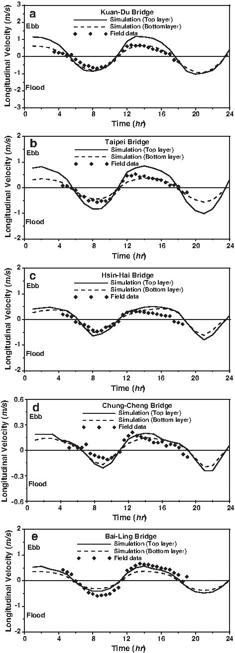
Comparison between observed and simulated time-series velocity on April 26, 2002, at (a) Kuan-Du Bridge, (b) Taipei Bridge, (c) Hsin-Hai Bridge, (d) Chung-Cheng Bridge, and (e) Bai-Ling Bridge. Note that simulation at top layer and bottom layer represents 0.2D and 0.8D (where D is water depth). Field data represent the depth averaged current.

Time-series salinity

Salinity distributions reflect the combined results of all processes, including density circulation and mixing processes. These in turn control the density circulation and modify the mixing processes. In the present study, the time-series data of salinity at Kuan-Du Bridge collected by the National Center for Ocean Research, Taiwan, were used for model validation. The salinities of open boundaries in the coastal sea were set to 35 ppt. The upstream boundary conditions at three tributaries (Tahan Stream, Hsintien Stream, and Keelung River) were also specified with daily freshwater discharges (Fig. 7a). The model was simulated starting from January 1, 2002. The simulated salinity time series compared favorably with the discrete salinity measurements on July 1–16, 2002, at Kuan-Du Bridge as shown in Fig. 7b. Absolute mean error and root-mean-square error are 3.72 and 5.37 ppt, respectively. The simulated salinities reproduce the pattern of observed salinity variations in a dynamic variation of salinity between 0 and 30 ppt over a tidal cycle. Overall, the model reflects the large dynamic variations of salinity over a tidal cycle, with decreasing values of mean salinity as freshwater discharge increases.

FIG. 7.

Comparison of observed and computed time-series salinity at Kuan-Du Bridge (a) discharges at three upstream boundaries and (b) salinity from July 1 to 16, 2002. Note that the field data of salinity was measured at 0.5 m below water surface.

Water quality distribution

The water quality conditions in the Danshuei River system have a conspicuous spatial trend with neither seasonal nor long-term temporal trend (Liu et al., 2003). Adjacent to the metropolitan Taipei City, it has been long believed that the spatial trend of the deteriorated water quality is mostly attributed to the wastewaters directly discharged into the river channels. Efforts were made successively to estimate the point and nonpoint source loadings via population information and analyses of field data by Liu et al. (2005) and Wang et al. (2005). The estimated pollutant loadings given by Wang et al. (2005) were adopted in the following water quality simulations.

The median freshwater discharges from 1987 to 2005 were adopted at the upstream boundaries, which were 12.8, 23.7, and 9.8 m³/s in the Tahan Stream, Hsintien Stream, and Keelung River, respectively. The five-constituent tide used in the mean tide simulation was employed at the ocean boundaries. Concentrations of water quality state variables at the river boundaries were estimated according to the assumption that the field water quality concentrations and river discharges follow the exponential relationship (C = aQ^b, where C is the water quality concentration, Q is the river discharge, and a and b are coefficients to be determined) (Hydroscience, Inc., 1976), whereas those at the ocean boundaries were specified according to the general observation data in the coastal sea measured by the Taiwan Ocean Research Institute (TORI). The regression results of the observed data, including concentrations of ammonium nitrogen, total nitrogen, total phosphorus, and dissolved oxygen, against the corresponding river discharges at three upstream boundaries are shown in Table 4. The positive/negative signs of the power in Table 4 mean that the concentrations at upstream boundaries increase/decrease with freshwater discharge. For example, the concentrations of ammonium nitrogen, total nitrogen, and total phosphorus increase when the freshwater discharges decrease. The initial conditions of water quality were set at 5.5, 0.5, 0.05, and 0.2 g/m³ for dissolved oxygen, ammonium nitrogen, total phosphorus, and total organic carbon, respectively.

Table 4.

Exponential Relationship Between Water Quality Concentrations and River Discharges at Three Upstream Boundaries

River	Dissolved oxygen	Ammonium nitrogen	Total nitrogen	Total phosphorus
Tahan Stream	6.18 × Q^0.028	0.73 × Q^−0.21	3.72 × Q^−0.11	0.075 × Q^−0.073
	R = 0.2	R = 0.43	R = 0.92	R = 0.24
Hsintien Stream	3.42 × Q^0.15	3.03 × Q^−0.27	7.51 × Q^−0.30	1.28 × Q^−0.52
	R = 0.54	R = 0.46	R = 0.67	R = 0.79
Keelung River	4.31 × Q^0.12	5.16 × Q^−0.53	3.34 × Q^−0.10	0.63 × Q^−0.38
	R = 0.85	R = 0.81	R = 0.53	R = 0.53

R is correlation coefficient.

The purpose of this median flow simulation was to see whether the water quality model is capable of generating the comparable spatial distribution of the water quality condition observed in situ.

The model parameters were initially estimated from the literature (Cerco and Cole, 1995). These were adjusted and tuned until a reasonable reproduction of field data at observation stations was achieved. Table 5 lists the coefficients adopted for water quality simulations.

Table 5.

Coefficients Used in Water Quality Model

Coefficients	Value	Unit
Oxygen-to-carbon ratio in respiration (AOC)	2.67	g-O₂/g-C
Mass of dissolved oxygen consumed per unit mass of ammonium nitrogen nitrified (AON)	4.57	g-O₂/g-N
Proportionality constant (K_ro)	2.0	—
Constant for temperature adjustment of DO reaeration rate (KT_r)	1.024	—
SOD	2.0	g-O₂/m²/day
Fraction of basal metabolized nitrogen by zooplankton produced as inorganic nitrogen (FNIZ)	0.05	—
Fraction of basal metabolized nitrogen by phytoplankton produced as inorganic nitrogen (FNI)	0.05	—
Fraction of predated zooplankton nitrogen produced as inorganic nitrogen (FNIPZ)	0.05	—
Fraction of predated phytoplankton nitrogen produced as inorganic nitrogen (FNIP)	0.05	—
Nitrification half-saturation constant for dissolved oxygen (KhNit_DO)	2.0	g-O₂/m³
Nitrification half-saturation constant for ammonium nitrogen (KhNit_N)	1.0	g-N/m³
Maximum nitrification rate at temperature TNit (Nit_m)	0.14	1/day
Optimum temperature for nitrification (TNit)	20	^°C
Effect of temperature above TNit on nitrification rate (KNit1)	0.0045	1/^°C²
Effect of temperature below TNit on nitrification rate (KNit2)	0.0045	1/^°C²
Sediment-water exchange flux of ammonium nitrogen (BFNH4)	0.05	g-N/m²/day
Sorption coefficient relating phosphate sorption to total suspended solid (K_PO4p)	0.1	g/m³
Fraction of basal metabolized phosphorus by zooplankton produced as inorganic phosphorus (FPIZ)	0.05	—
Fraction of basal metabolized phosphorus by phytoplankton produced as inorganic phosphorus (FPI)	0.05	—
Fraction of predated zooplankton phosphorus produced as inorganic phosphorus (FPIPZ)	0.2	—
Fraction of predated phytoplankton phosphorus produced as inorganic phosphorus (FPIP)	0.2	—
Sediment-water exchange flux of dissolved phosphate (BFPO4d)	0.005	g-P/m²/day
Fraction of predated zooplankton carbon produced as refractory particulate organic carbon (FCRPZ)	0.35	—
Fraction of predated phytoplankton carbon produced as refractory particulate organic carbon (FCRP)	0.35	—
Fraction of predated zooplankton carbon produced as labile particulate organic carbon (FCLPZ)	0.5	—
Fraction of predated phytoplankton carbon produced as labile particulate organic carbon (FCLP)	0.5	—
Minimum dissolution rate of refractory particulate organic carbon (K_RC)	0.005	1/day
Constant that relates dissolution of refractory particulate organic carbon to phytoplankton biomass (K_RCalg)	0.1	1/day per g-C/m³
Effect of temperature on hydrolysis of particulate organic matter (KT_HDR)	0.069	1/^°C
Reference temperature for hydrolysis of particulate organic matter (TR_HDR)	20.0	^°C
Minimum dissolution rate of labile particulate organic carbon (K_LC)	0.075	1/day
Constant that relates dissolution of labile particulate organic carbon to phytoplankton biomass (K_LCalg)	0.1	1/day per g-C/m³
Fraction of predated zooplankton carbon produced as dissolved organic carbon (FCDPZ)	0.1	—
Fraction of predated phytoplankton carbon produced as dissolved organic carbon (FCDP)	0.1	—
Fraction of basal metabolized carbon by zooplankton produced as dissolved organic carbon (FCDZ)	0.05	—
Half-saturation constant of dissolved oxygen for zooplankton excretion of dissolved organic carbon (KHRZ)	0.5	g-O₂/m³
Fraction of basal metabolized carbon by phytoplankton produced as dissolved organic carbon at infinite dissolved oxygen concentration (FCD)	0.05	—
Half-saturation constant of dissolved oxygen for phytoplankton excretion of dissolved organic carbon (KHR)	0.5	g-O₂/m³
Oxic respiration half-saturation constant for dissolved oxygen (KhOR_DO)	0.5	g-O₂/m³
Minimum respiration rate of dissolved organic carbon (K_DC)	0.34	1/day
Constant that relates respiration of dissolved organic carbon to phytoplankton biomass (K_DCalg)	0.1	1/day per g-C/m³
Effect of temperature on mineralization of dissolved organic matter (KT_MNL)	0.069	1/°C
Reference temperature for mineralization of dissolved organic matter (KhDN_N)	0.1	g-N/m³
Ratio of denitrification rate to oxic dissolved organic carbon respiration rate (AANOX)	0.5	—

SOD, sediment oxygen demand.

The model was simulated for 20 days, but the modeling results at the last 5 days were taken as an average to calculate water quality conditions. The longitudinal water quality distributions predicted by the water quality model under median flow condition for the Danshuei River-Tahan Stream, Hsintien Stream, and Keelung River are shown in Figs. 8 –10, respectively. Water quality distributions of the dissolved oxygen, ammonium nitrogen, total phosphorus, and total organic carbon concentrations along the river channels are presented in the figures, together with the median values of observations at monitoring stations from 1987 to 2005. Figure 8a reveals that both the model-predicted and observed median values of dissolved oxygen concentration along the Tahan Stream show a decreasing trend from Fu-Chou Bridge to Hsin-Hai Bridge. In the lower estuary, the dissolved oxygen concentrations increase toward the river mouth as a result of seawater dilution. The lowest dissolved oxygen concentration occurs in the river reach from Hsin-Hai Bridge to Kuan-Du Bridge. Total organic carbon, ammonium nitrogen, and total phosphorous show the same spatial trends along the river channel from Tahan Stream to Danshuei River. The concentrations increase in the downstream direction from Fu-Chou Bridge, reach a maximum at the Hsin-Hai Bridge, and then gradually decrease toward the river mouth. Maximum concentrations of all the three occur at the Hsin-Hai Bridge, and the dissolved oxygen level is severely depressed in the river reach downstream. The figure shows that the model generally captured the spatial trends of the observed longitudinal distributions but underestimated the maximum concentration of total phosphorus (Fig. 8c).

FIG. 8.

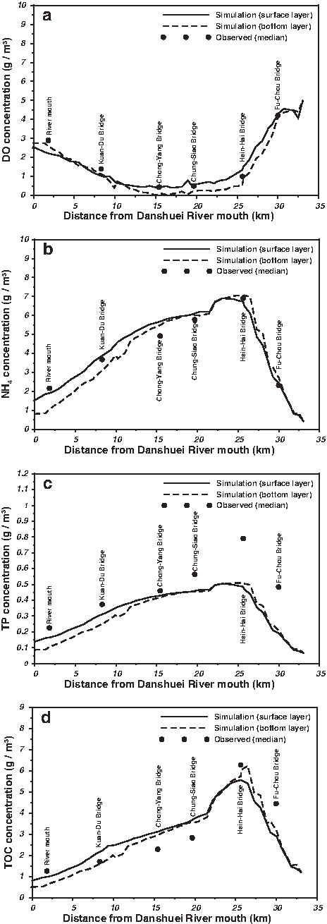
Water quality distribution along the Danshuei River and Tahan Stream under median flow condition: (a) dissolved oxygen, (b) ammonium nitrogen, (c) total phosphorus, and (d) total organic carbon.

FIG. 9.

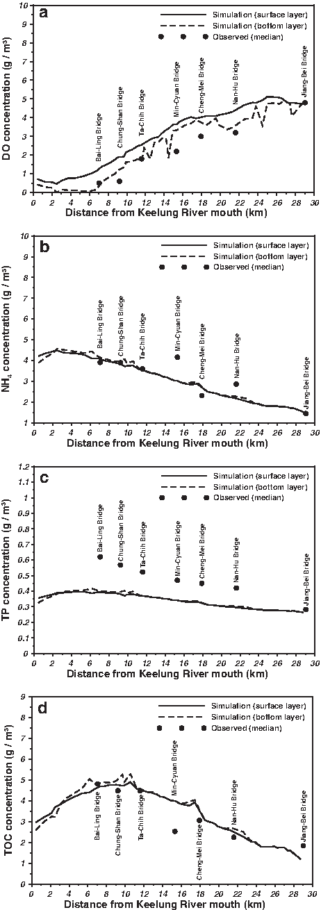
Water quality distribution along the Hsintien Stream under median flow condition: (a) dissolved oxygen, (b) ammonium nitrogen, (c) total phosphorus, and (d) total organic carbon.

FIG. 10.

Water quality distribution along the Keelung River under median flow condition: (a) dissolved oxygen, (b) ammonium nitrogen, (c) total phosphorus, and (d) total organic carbon.

Figure 9 shows the longitudinal water quality distributions along the Hsintien Stream. Both the observation data and model predictions show that the water quality conditions degrade as it approaches the river mouth where it joins the main stem Danshuei River, the dissolved oxygen decreases, and the organic carbon, ammonium nitrogen, and total phosphorus increase monotonically. The underestimation of total phosphorus is similar to that in the river channel from Tahan Stream to Danshuei River. The reason may be that the ungauged distributed total phosphorus loads cannot be really estimated.

The longitudinal water quality distribution along the Keelung River (Fig. 10) shows that there were significant pollution loadings discharged into the river section around Bai-Ling Bridge, where the highest concentrations of pollutants and lowest dissolved oxygen in the Keelung River were observed. The results also indicate that the total phosphorus was underestimated.

Sensitivity Analysis for Water Quality Model

Sensitivity analysis is a powerful methodology that can be applied to improve the understanding of the present water quality distributions in the estuaries due to the changing of major coefficients. The maximum rate is used to quantify the results of sensitivity analysis. It means that the maximum values were determined by the following formula: \documentclass{aastex} \usepackage{amsbsy} \usepackage{amsfonts} \usepackage{amssymb} \usepackage{bm} \usepackage{mathrsfs} \usepackage{pifont} \usepackage{stmaryrd} \usepackage{textcomp} \usepackage{portland, xspace} \usepackage{amsmath, amsxtra} \pagestyle{empty} \DeclareMathSizes {10} {9} {7} {6} \begin{document} \begin{align*} {\rm MR} = \frac {\mid C_ {\rm base} - C_ {\rm sens} \mid} {C_ {\rm base}} \times 100 \% \tag {8} \end{align*} \end{document}

where C_base is the water quality state variables for the base simulations, shown in Figs. 8 –10, and C_sens is the water quality state variables for the sensitivity simulations.

Sediment oxygen demand

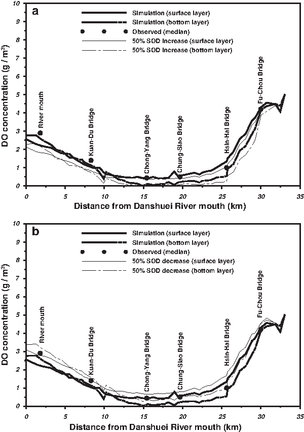
The solute flux across the sediment–water interface influences various aspects of the water quality of inland and coastal waters. One of the most prominent interactions is the flux of dissolved oxygen from the water body into the sediment, which is termed sediment oxygen demand (SOD) (Di Toro, 2001). The SOD may be a major contributor to the overall oxygen budget of inland waters. Therefore, the effect of SOD on the dissolved oxygen distributions was investigated with two alternative cases: one involves validated value listed in Table 5 plus 50% SOD, and the other involved validated value minus 50% SOD.

Figure 11 presents the modeling result of sensitivity analysis for dissolved oxygen distributions in the Danshuei River-Tahan Stream with increasing and decreasing SOD. Table 6 summarizes the sensitivity results including the Danshuei River-Tahan Stream, Hsintien Stream, and Keelung River. It shows that an increase in the SOD results in a decrease in the dissolved oxygen at the surface and bottom layers (Fig. 11a). The maximum rates for decreasing dissolved oxygen are 47.9% and 94.2% at the surface and bottom layers, respectively, in the Danshuei River-Tahan Stream. The decrease in SOD increases the dissolved oxygen at the surface and bottom layers in the Danshuei River-Tahan Stream presented in Fig. 11b. The maximum rates of increasing dissolved oxygen are 67.5% and 118.0% at the surface and bottom layers, respectively, in the Danshuei River-Tahan Stream (Table 6). The modeling results indicate that the SOD has a significant impact on the distribution of dissolved oxygen concentration in the Danshuei River estuarine system.

FIG. 11.

Sensitivity analyses simulating with (a) increasing SOD and (b) decreasing SOD for the dissolved oxygen distribution in the Danshuei River-Tahan Stream. SOD, sediment oxygen demand.

Table 6.

Results of Sediment Oxygen Demand Sensitivity Analysis

River	SOD sensitivity simulation	Maximum rate of dissolved oxygen concentration for surface layer (%)	Maximum rate of dissolved oxygen concentration for bottom layer (%)
Danshuei River-Tahan Stream	Decreasing 50% SOD	67.5	118.0
	Increasing 50% SOD	−47.9	−94.2
Hsintien Stream	Decreasing 50% SOD	37.1	118.7
	Increasing 50% SOD	−28.5	−72.8
Keelung River	Decreasing 50% SOD	69.7	121.1
	Increasing 50% SOD	−28.27	−97.25

Minus and plus values represent decreasing and increasing dissolved oxygen concentrations, respectively.

Sediment–water exchange flux of ammonium nitrogen (BFNH4)

In model validation of water quality, an external input of nutrients in the form of benthic flux of ammonium nitrogen was needed to reproduce the observed ammonium nitrogen in the tidal river. The results from a sensitivity analysis with increasing 50% BFNH4 and decreasing 50% BFNH4 based on the validated value (BFNH4) listed in Table 5 are presented in Fig. 12. It indicates that the increase of BFNH4 results in increasing ammonium nitrogen concentration at the surface and bottom layers. Table 7 summarizes the sensitivity results for BFNH4 in the estuarine system. The maximum rates of increasing BFNH4 are 2.8% and 3.6% at the surface and bottom layers, respectively, in the Danshuei River-Tahan Stream, whereas the maximum rates for decreasing BFNH4 are 5.1% and 14.1% at the surface and bottom layers, respectively. The small maximum rates are also shown for the Hsintien Stream and Keelung River (Table 7). It means that the sediment–water exchange flux of ammonium nitrogen (BFNH4) has a slight influence on the ammonium nitrogen concentration in the estuarine system.

FIG. 12.

Sensitivity analyses simulating with (a) increasing sediment–water exchange flux of ammonium nitrogen (BFNH4) and (b) decreasing BFNH4 for ammonium nitrogen distribution in the Danshuei River-Tahan Stream.

Table 7.

Results of Sensitivity Analysis for Sediment–Water Exchange Flux of Ammonium Nitrogen (BFNH4)

River	BFNH4 sensitivity simulation	Maximum rate of dissolved oxygen concentration for surface layer (%)	Maximum rate of dissolved oxygen concentration for bottom layer (%)
Danshuei River-Tahan Stream	Decreasing 50% BFNH4	−5.1	−14.1
	Increasing 50% BFNH4	2.8	3.6
Hsintien Stream	Decreasing 50% BFNH4	−2.3	−3.1
	Increasing 50% BFNH4	0.6	0.3
Keelung River	Decreasing 50% BFNH4	−3.2	−3.0
	Increasing 50% BFNH4	2.3	3.7

Minus and plus represent decreasing and increasing dissolved oxygen concentrations, respectively.

Freshwater discharge

The effects of changes in river discharge on nutrients and biological processes have been widely reported (Lin et al., 2008; van Beusekom et al., 2008); therefore, the sensitivity analyses were conducted to investigate the effects of river discharge on the water quality conditions. The low river discharge (Q₇₅ flow) was adopted to compare with the results for median freshwater discharge (base simulation). The Q₇₅ freshwater discharge means that the flow is equaled or exceeded 75% of time. For the Q₇₅ flow, the discharge at the tidal limits of the three major tributaries, Tahan Stream, Hsintien Stream, and Keelung River, are 3.36, 14.23, and 3.33 m³/s, respectively. Water quality conditions at the river boundaries were calculated based on the equations listed in Table 4.

Figure 13 presents the sensitivity analyses for the dissolved oxygen, ammonium nitrogen, and total phosphorus in the Danshuei River-Tahan Stream. It reveals that low freshwater discharges significantly lead to lower dissolved oxygen and higher nutrients compared with the results for median freshwater discharge. Table 8 shows the results of sensitivity analysis for freshwater discharge in the estuarine system. The maximum rates of decreasing freshwater discharge are 61.0%, 144.1%, and 95.7% for the dissolved oxygen, ammonium nitrogen, and total phosphorus at the surface layer, respectively, in the Danshuei River-Tahan Stream, whereas the maximum rates for decreasing freshwater discharge are 95.5%, 142.4%, and 93.6% at the bottom layer. The high maximum rates also appear in the Hsintien Stream and Keelung River (Table 8). The results indicate that freshwater discharges at upstream boundaries have significant impacts on water quality distributions in the estuarine system.

FIG. 13.

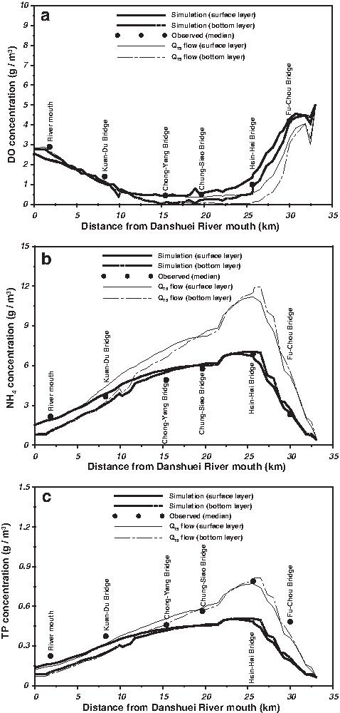
Sensitivity analyses simulating with Q₇₅ freshwater discharge in the Danshuei River-Tahan Stream: (a) dissolved oxygen, (b) ammonium nitrogen, and (c) total phosphorus.

Table 8.

Results of Sensitivity Analysis for Decreasing Freshwater Discharge (Q₇₅)

	Maximum rate of dissolved oxygen concentration for surface layer (%)			Maximum rate of dissolved oxygen concentration for bottom layer (%)
River	Dissolved oxygen	Ammonium nitrogen	Total phosphorus	Dissolved oxygen	Ammonium nitrogen	Total phosphorus
Danshuei River-Tahan stream	−61.0	144.1	95.7	−95.5	142.4	93.6
Hsintien stream	−61.3	48.1	34.3	−96.7	63.6	42.3
Keelung river	−53.3	99.3	48.9	−100.0	100.3	48.9

Minus and plus values represent decreasing and increasing dissolved oxygen concentrations, respectively.

Conclusions

A three-dimensional water quality model based on the hydrodynamic model was developed and applied to the Danshuei River estuarine system for simulating water quality conditions including dissolved oxygen, ammonium nitrogen, total phosphorus, and total organic carbon. The hydrodynamic and water quality model has been validated with observational tidal range, water surface elevation, velocity, salinity, and water quality state variables. The simulated results using the three-dimensional hydrodynamic model revealed that the computed tidal range, water surface elevation, velocity, and salinity were well reproduced with observed data. The bottom topography, roughness height, and diffusivities in horizontal and vertical directions are of crucial importance, as these affect the hydrodynamic characteristics. The modeling results using the water quality model indicated that the computed water quality state variables including dissolved oxygen, ammonium nitrogen, total phosphorus, and total organic carbon caught the trends of observed data. More efforts should be taken to estimate the pollution loadings that significantly affect the water quality distributions in the Danshuei River estuarine system.

The model sensitivity analyses provide further insight into the understanding of dissolved oxygen and nutrient distributions in the estuarine system. Model sensitivity analyses for SOD, BFNH4, and freshwater discharge were conducted with the validated model. The results show that maximum rates of dissolved oxygen concentration with increasing and decreasing SOD are higher than the maximum rates of ammonium nitrogen concentration with increasing and decreasing BFNH4. It means that SOD plays an important role in affecting the dissolved oxygen distributions in the Danshuei River estuarine system. Median and low freshwater discharges were adopted to probe the effects on the water quality characteristics. It reveals that low freshwater discharges significantly lead to lower dissolved oxygen and higher nutrients compared with the results using median freshwater discharge. The model will provide a useful tool for developing management practices and protecting water quality in the Danshuei River estuarine system in the future.

Footnotes

Acknowledgments

This study was supported in part by the Taiwan's National Science Council (Grant Nos. 96-2628-E-239-012-MY3 and 98-2625-M-239-001). This financial support is greatly appreciated. The authors also thank the Taiwan Water Resources Agency, Central Weather Bureau, and Environmental Protection Administration for providing the observed data used in the model validation. The authors sincerely thank three anonymous reviewers for their valuable comments.

Author Disclosure Statement

No competing financial interests exist.

References

Brush

M.J.

, Nixon

S.W.

2010. Modeling the role of macroalgae in a shallow sub-estuary of Narragansett Bay, RI (USA) Ecol. Model., 221:1065.

Casulli

, Walters

R.V.

2000. An unstructured grid, three-dimensional model based on the shallow water equations. Int. J. Numer. Methods Fl., 32:331.

Cerco

C.F.

, Cole

T.M.

1993. Three-dimensional eutrophication model of Chesapeake Bay. J. Environ. Eng. ASCE, 119:1006.

Cerco

C.F.

, Cole

T.M.

1995. User's Guide to the CE-QUAL-ICM Three-Dimensional Eutrophication Model: Release Version 1.0Technical Report EL-95-15, US Army Corps of Engineers, Waterways Experiment Station, Vicksburg, MS.

Chau

K.W.

2005. An unsteady three-dimensional eutrophication model in Tolo harbour, Hong Kong. Mar. Pollut. Bull., 51:1078.

Di Toro

D.M.

2001. Sediment Flux Modeling. New York: Wiley.

Foreman

M.G.G.

, Henery

R.F.

, Walters

R.A.

, Ballabtyne

V.A.

1993. A finite element model for tides and resonance along the north coast of British Columbia. J. Geophys. Res., 98:2509.

Garcia

, Juanes

J.A.

, Alvarez

, Revilla

J.A.

, Medina

2010. Assessment of the response of a shallow macrotidal estuary to changes in hydrological and wastewater inputs through numerical modeling. Ecol. Model., 221:1194.

Hsieh

H.L.

, Fan

L.F.

, Chen

C.P.

, Wu

J.T.

, Liu

W.C.

2010. Effect of semidiurnal tidal circulation on the distribution of holo- and meroplankton in a subtropical estuary. J. Plankton Res., 32:829.

10.

Hsu

M.H.

, Kuo

A.Y.

, Kuo

J.T.

, Liu

W.C.

1999. Procedure to calibrate and verify numerical models of estuarine hydrodynamics. J. Hydraul Eng. ASCE, 125:166.

11.

Hydroscience, Inc. 1976. Water Quality Analysis of Potomac River. Report to the Interstate Commission of Potomac River Basin: New Jersey.

12.

Lessin

, Raudsepp

2006. Water quality assessment using integrated modeling and monitoring in Narva Bay, Gulf of Finland. Environ. Model. Assess., 11:315.

13.

Lin

, Xie

, Pietrafesa

L.J.

, Ramus

J.S.

, Paerl

H.W.

2007. Water quality gradients across Albemarle-Pamlico estuarine system: Seasonal variations and model applications. J. Coastal Res., 23:213.

14.

Lin

, Xie

, Pietrafesa

L.J.

, Xu

, Woods

, Mallin

M.A.

, Durako

M.J.

2008. Water quality responses to simulated flow and nutrient reductions in the Cape Fear River Estuary and adjacent coastal region, North Carolina. Ecol. Model., 212:200.

15.

Liu

S.Y.

, Liu

W.C.

, Hsu

M.H.

, Kuo

A.Y.

2003. Recent water quality conditions in Danshuei River estuarine system. Taiwan Water Conserv., 51:43(In Chinese).

16.

Liu

W.C.

, Hsu

M.H.

, Kuo

A.Y.

2001a. Investigation of long-term transport in Tanshui Estuary, Taiwan. J. Waterw. Port Coast. Ocean Eng. ASCE, 127:61.

17.

Liu

W.C.

, Hsu

M.H.

, Kuo

A.Y.

2007. Three-dimensional hydrodynamic and salinity transport modelling of Danshuei River estuarine system and adjacent coastal sea, Taiwan. Hydrol. Process., 21:3057.

18.

Liu

W.C.

, Hsu

M.H.

, Kuo

A.Y.

, Li

M.H.

2001b. A modeling study of water quality in main channel and estuarine wetland. J. Environ. Sci. Health Part A, 36:641.

19.

Liu

W.C.

, Liu

S.Y.

, Hsu

M.H.

, Kuo

A.Y.

2005. Water quality modeling to determine minimum instream flow for fish survival in tidal rivers. J. Environ. Manage., 76:293.

20.

Lung

W.S.

, Nice

A.J.

2007. Eutrophication model for the Patuxent Estuary: Advances in predictive capabilities. J. Environ. Eng. ASCE, 133:917.

21.

McGlathery

K.J.

, Sundback

, Anderson

I.C.

2007. Eutrophication in shallow coastal bay and lagoons: the role of plants in the coastal filter. Mar. Ecol. Prog. Ser., 348:1.

22.

Park

, Jung

H.S.

, Kim

H.S.

, Ahn

S.M.

2005. Three-dimensional hydrodynamic-eutrophication model (HEM-3D): application to Kwang-Yang Bay, Korea. Mar. Environ. Res., 60:171.

23.

Timmermann

, Markager

, Gustafsson

K.E.

2010. Streams or open sea? Tracing sources and effects of nutrient loadings in a shallow estuary with a 3D hydrodynamic-ecological model. J. Mar. Syst., 82:111.

24.

van Beusekom

J.E.E.

, Weigelt-Krenz

, Martens

2008. Long-term variability of winter nitrate concentrations in the Northern Wadden Sea driven by freshwater discharge, decreasing riverine loads and denitrification. Helgoland Mar. Res., 62:49.

25.

Wang

C.F.

2005. Modeling Study of Water Quality and Ecological System in the Danshuei River Estuary. Ph.D. Dissertation, Department of Bioenvironmental Systems Engineering. National Taiwan University: Taipei, Taiwan, 171.

26.

Wang

C.F.

, Hsu

M.H.

, Kuo

A.Y.

2004. Residence time of Danshuei River estuary, Taiwan. Estuar. Coast. Shelf Sci., 60:381.

27.

Wool

T.A.

, Davie

S.R.

, Rodriguez

H.N.

2003. Development of three-dimensional hydrodynamic and water quality models to support total maximum daily load decision process for the Neuse River Estuary, North Carolina. J. Water Resour. Plan. Manage. ASCE, 129:295.

28.

Zhang

Y.L.

, Baptista

A.M.

, Myers

E.P.

2004. A cross-scale model for 3D baroclinic circulation in estuary-plume-shelf systems: I. Formulation and skill assessment. Cont. Shelf Res., 24:2187.

29.

Zheng

L.Y.

, Cheng

C.S.

, Zhang

F.Y.

2004. Development of water quality model in the Satilla River Estuary, Georgia. Ecol. Model., 178:457.