




Abstract
Abstract
Stability and accuracy of retrieving the aerosol size-distribution by using the linear-regression (LR), genetic algorithm (GA), and annealing genetic algorithm (AGA) were studied in detail. It was found that by using the AGA, retrieval results are quite stable and accurate; using the GA, stability and accuracy of the retrieval results decreased mildly but were still acceptable; and using the LR, retrieval results were too unstable to be acceptable. This conclusion is verified by both of the numeric simulation and the experiment.
Introduction
Suppose that the initial radiance at wavelength λ is I0(λ), and after passing through the atmosphere it becomes I1(λ), according to the Lambert-Beer law it has (Zuo and Yang, 2007).
where τ(λ) is the atmospheric optical depth of the aerosol and τoth(λ) is the total optical depths of other extinction factors in the air. τ(λ) can be expressed as (Hulst, 1957).
in which r is the radius of the aerosol; rmin and rmax are the lower and upper limits of the radius respectively; Q(r, λ), which can be calculated by using Mie scattering theory (Hulst, 1957), is the extinction efficiency of the particle whose radius is r; and n(r) is the undetermined aerosol size-distribution. Theoretically, if τ(λ) is known, n(r) can be retrieved by solving equation (2). So far, there are two models to retrieve n(r), one is the dependent-model and the other is the independent-model.
The independent-model is more objective and more universal than the dependent model (Kulkarni and Wang, 2006). According to the idea of the independent-model, the radius section [rmin, rmax] is divided into M sub-sections, and in every sub-section n(r) is supposed to be a constant ni. Then, equation (2) can be rewritten as
where ri is the average radius of particles in the i th sub-section. In this way, the problem is converted into solving a matrix equation. It seems that by solving equation (3), ni can be retrieved with the number of the wavelengths being greater than or equal to M. However, usually the Mie matrix Q(ri, λ) is ill-conditioned, which would introduce large error and instability into the retrieval results. In order to solve this problem, many techniques have been attempted. Previously, the linear-regression (LR) method was used, which is quite simple. Afterward, some optimal algorithms were applied in the retrieval, which can get more stable and accurate results.
This article will compare the retrieval stability and accuracy of the LR and two optimal algorithms—the genetic algorithm (Kim et al., 2007) (GA) and annealing genetic algorithm (AGA)—in detail. First, the GA and AGA are briefly introduced; then, the retrieval stability and accuracy of LR, GA, and AGA are compared by numerical simulation; afterward, the accuracy is further compared by the actual measurement; at last, the main results are summarized.
The GA and the AGA
GA is a class of probabilistic optimization algorithms that are inspired by biological evolution process. GA is particularly useful for hard problems where little is known about the underlying search space. The process of GA includes initialization, selection, mutation, variation, and so on. Although GA is not guarantee that always gives the optimum solution, it usually gives an approximately good solution in a short time.
However, the GA, although it is called the “global optimal algorithm,” is easy to be trapped in local optimum (Kim et al., 2007; Ye et al., 1999), which would also influence the stability and accuracy of the retrieval results. In recent years, the AGA was proposed (Yu et al., 2000; Sun, 2010), which combined the advantages of GA with those of simulated annealing algorithm and was more easy to search for the global optimum. It is expected to get more stable and more accurate retrieval results by using AGA.
Numeric Simulation
In the simulation, four supposed size-distributions serve as the standard size-distributions. Substituting the standard size-distributions into equation (3), the values of the τ(λ) can be obtained. Based on the simulated value of τ(λ), the aerosol size-distribution can be retrieved by using the LR, GA, and AGA, respectively. Then, the stability and accuracy of the three algorithms can be reflected by the correlation coefficients between the retrieved size-distributions and the standard size-distributions.
Standard size-distributions and the related simulation conditions
The four supposed standard size-distributions are shown in Fig. 1. Fig. 1a is a Junge distribution with its index −1.5, Fig. 1b is a Gauss distribution, Fig. 1c is a bimodal distributions, and Fig. 1d is triple-peak distribution. The radius range is 0.1–5 μm, which is divided into 50 sub-sections (therefore, at least 50 wavelengths are needed in the retrieval of the size-distribution), the complex refractive index of the aerosol is supposed to be 1.306-0.001i, and the 50 wavelengths used to measure values of the τ(λ)are equidistantly selected in the spectrum range of 300–900 nm.
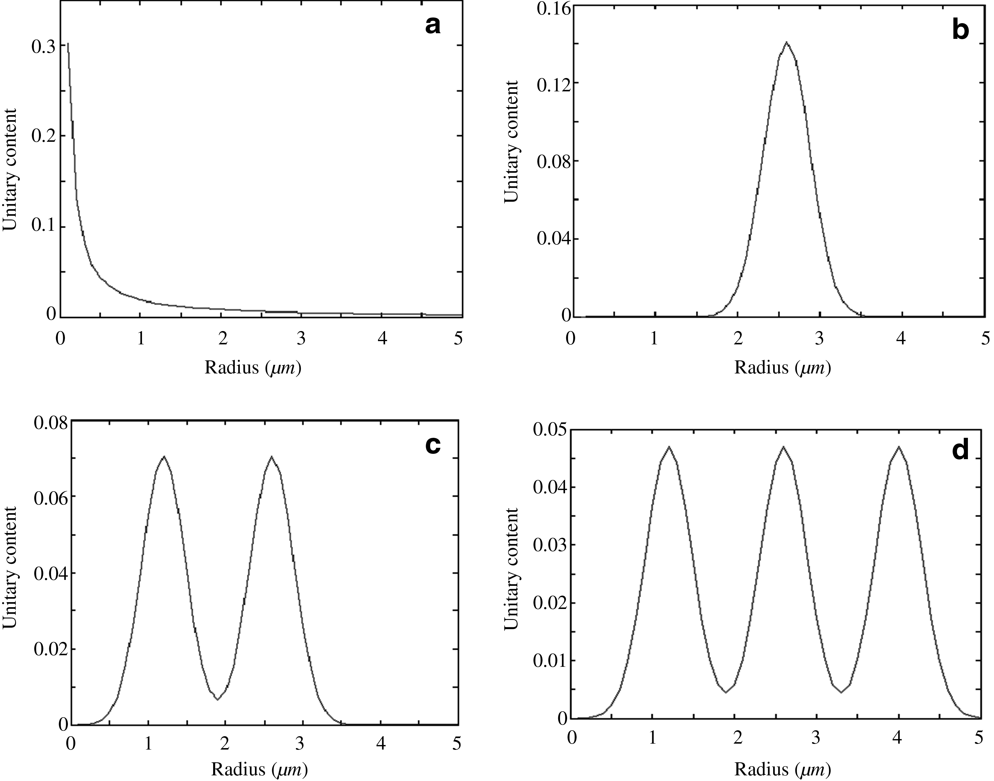
Standard size-distributions.
The realization of the LR, GA, and AGA
The LR is realized by the LR command of the software of MATLAB, that is lsqnonneg(p1, p2), and the meaning of the parameter p1 and p2 can refer to the help file of MATLAB.
The program of GA is compiled by using MATLAB, and the evolution conditions of GA are 40 initial groups of random computer-generated size-distributions, a float-point coding method, random crossing points, random mating ratios, a 0.2% variant ratio, and the fitness function is
where relat[τa (λ), τt (λ)] means the relative coefficient between the optical depth (τa(λ)) of the standard size-distribution and the optical depth (τt(λ)) of the transitional size-distribution groups. In the evolution process, when the groups keep stable, the results will be output.
The program of AGA is the modification of the program of GA, that is, embedding the Simulated Annealing technique into the GA program. In the evolution process, the offspring will compete with the parents and be accepted according to the Boltzmann law; in this way, the probability of the results that have been trapped in the local optimum can be decreased. Concretely, the evolution conditions of the AGA are the same as those of the GA; and the annealing conditions of AGA are an initial temperature of 103 K, a cooling speed of 0.99, and a terminating temperature of 0.01 K.
The concrete simulation process
The concrete simulation process is illustrated by taking the Junge distribution as an example. The values of the τ(λ)of the Junge distribution are first calculated by using equation (3) and then the following steps are taken.
• Retrieve the distribution 40 times by using three algorithms respectively without adding any errors to τ(λ), and, of course, every algorithm can get 40 retrieval results. Then, calculate the correlation coefficients between the retrieved size-distributions and the standard distributions. • Add 0%–1% random errors to τ(λ) and retrieve the size-distribution by using the three algorithms respectively. This process will be performed 40 times, and, of course, every algorithm can get 40 retrieval results. Then, calculate the correlation coefficients between the retrieved size-distributions and the standard distributions. • Add 0%–2% random errors to τ(λ) and retrieve the size-distribution by using the three algorithms respectively. This process will be performed 40 times, and, of course, every algorithm can get 40 retrieval results. Then, calculate the correlation coefficients between the retrieved size-distributions and the standard distributions. • Add 0%–4% random errors to τ(λ) and retrieve the size-distribution by using the three algorithms respectively. This process will be performed 40 times, and, of course, every algorithm can get 40 retrieval results. Then, calculate the correlation coefficients between the retrieved size-distributions and the standard distributions. • The simulation of the Gauss distribution, bimodal distribution, and the triple-peak distribution are repeating the whole process just described.
The results of the simulation
The correlation coefficients between the retrieved size-distributions and the standard size-distributions are shown in Figs. 2–4 (sorted in ascending order), which can reflect the stability and accuracy of the three algorithms.
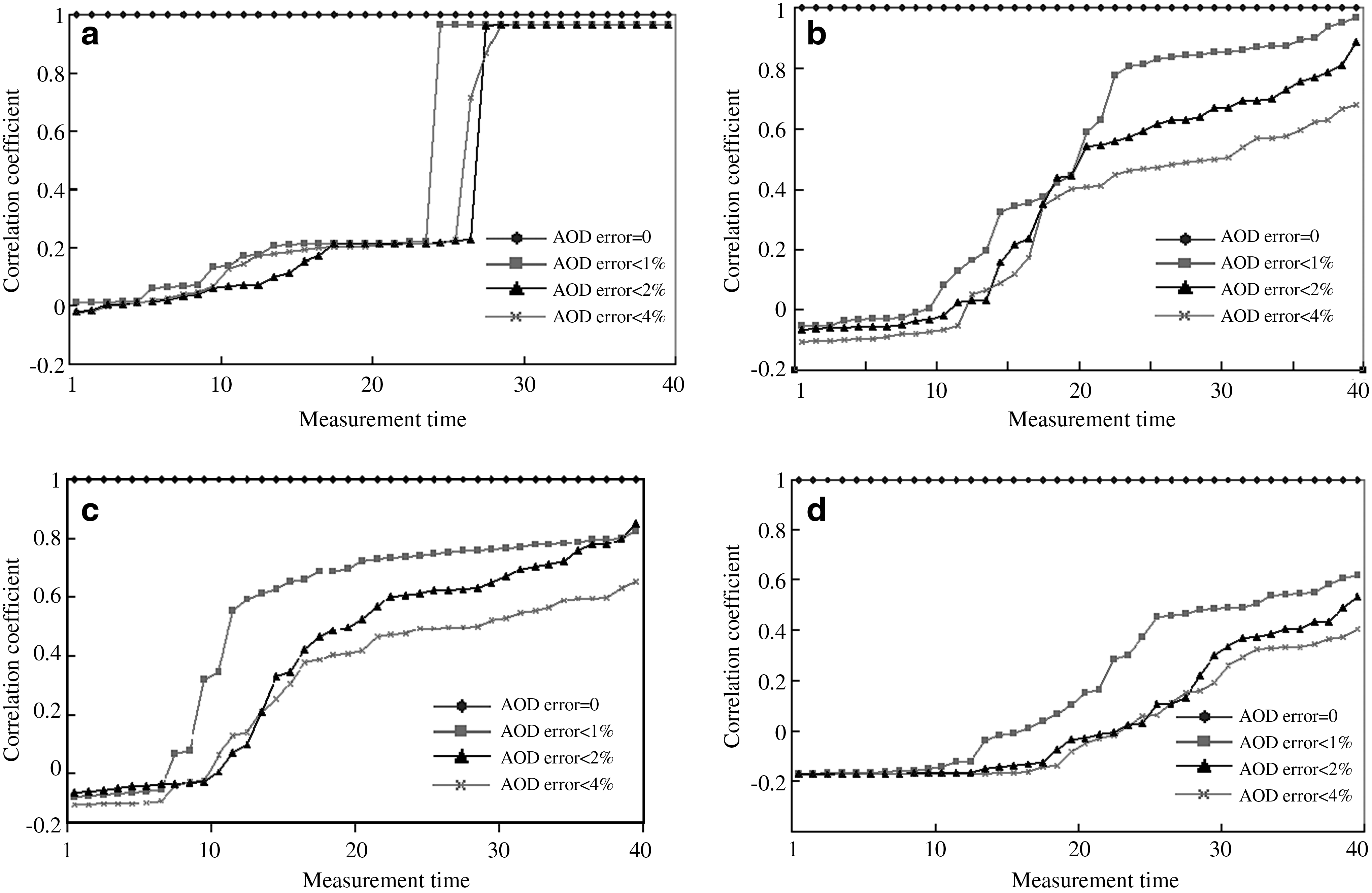
Correlation coefficients between the retrieval results from linear-regression and the standard size-distributions (sorted in ascending order)
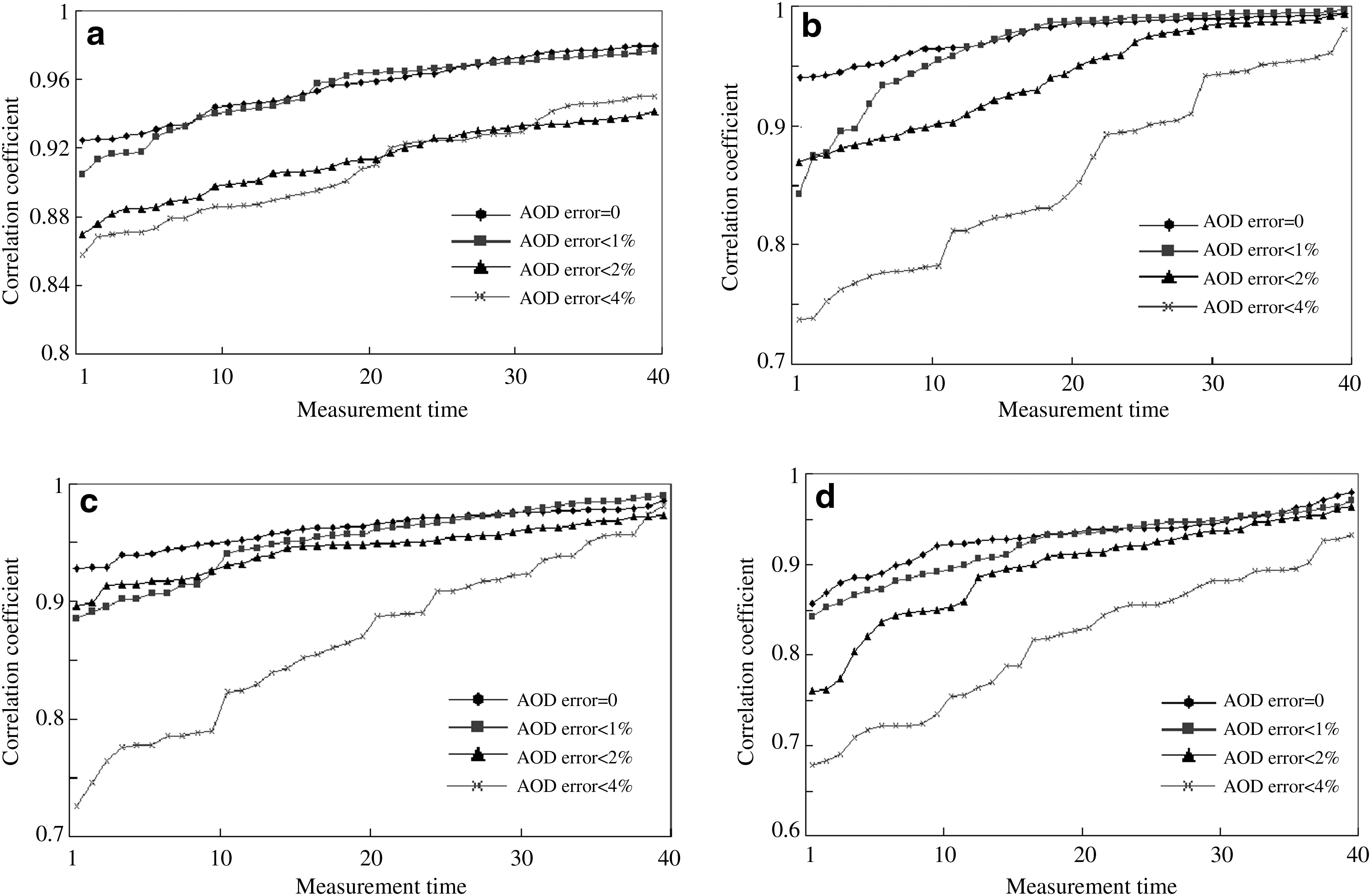
Correlation coefficients between the retrieval results from GA and the standard size-distributions (sorted in ascending order)
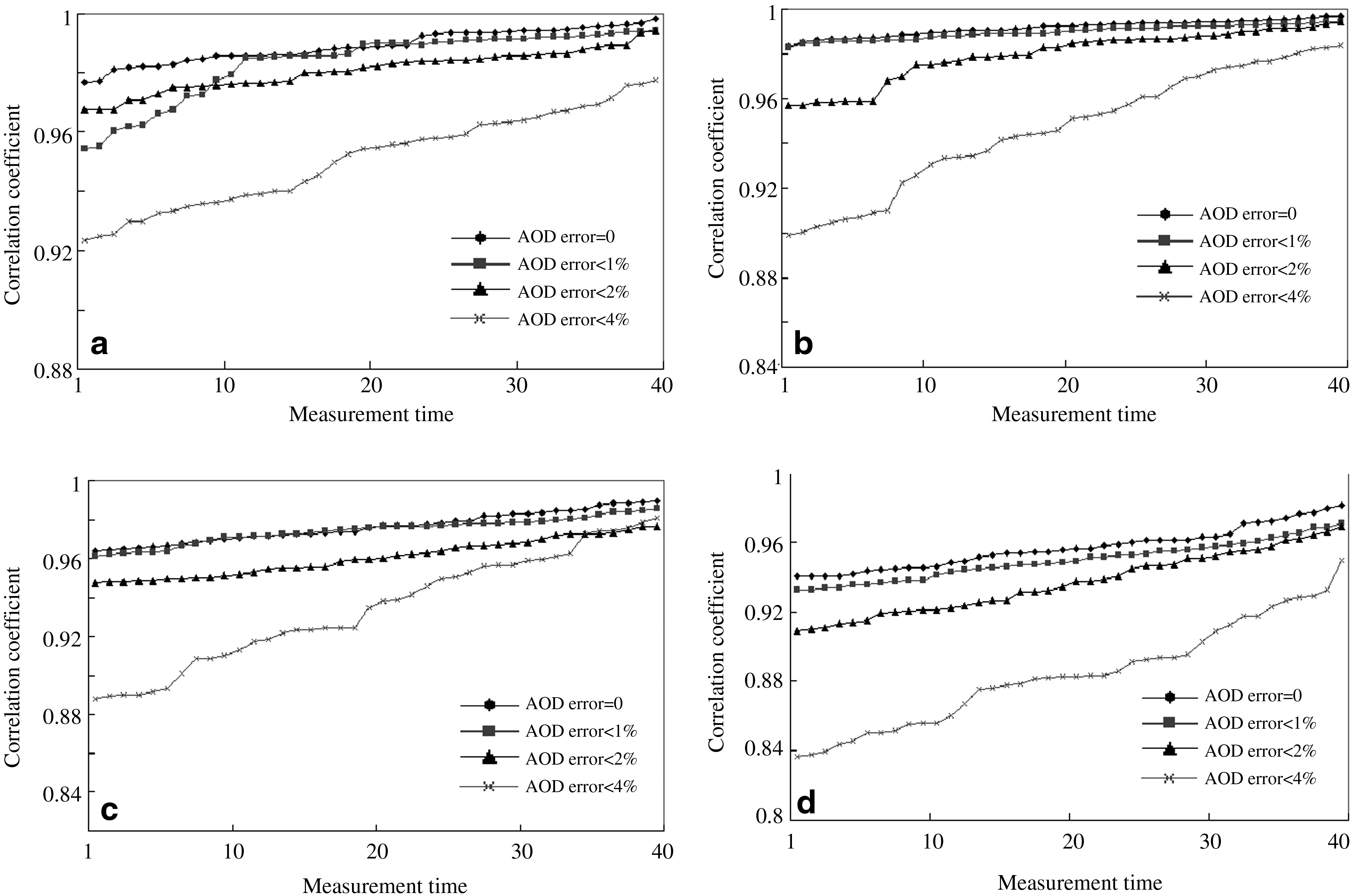
Correlation coefficients between the retrieval results from AGA and the standard size-distributions (sorted in ascending order)
Fig. 2 shows the correlation coefficients between the retrieval results from LR and the standard size-distributions. It can be seen that to all the distributions, when errors of τ(λ) is 0, the retrieval results from the LR are accurate and stable completely, and the correlation coefficients are 1. When the upper limit of the errors of τ(λ) reach 1%, the stability of the retrieval results decrease sharply, and even the negative correlation coefficients appear. When the upper limit of the errors of τ(λ) reach 2% and 4%, the retrieval results become much more unstable.
Fig. 3 shows the correlation coefficients between the retrieval results from GA and the standard size-distributions. It can be seen that when the errors of the τ(λ) are 0, the results are quite stable and accurate, but the correlation coefficients are all slightly smaller than 1 and there are tiny differences among the correlation coefficients, which may be due to the differences of the concrete initial groups and the cross points of very retrieval. When the error is increased, the stability and accuracy are mildly decreased. However, generally speaking, even if the errors reach 4%, the retrieval results are still acceptable.
Fig. 4 shows the correlation coefficients between the retrieval results from AGA and the standard size-distributions. It can be seen that the results from AGA are very stable and quite accurate, even if the upper limit of the errors reach 4%, the minimum correlation coefficient exceeds 0.8.
Experimental Verification
The retrieval accuracy of the three algorithms is further verified by retrieving the size-distribution of the polystyrene particles in water. First, the size-distributions of two types of spherical polystyrene particles are measured precisely by using a microscope (JSM-5900LV) as the reference standards, and the results are shown by the histograms in Fig. 5. Then, the τ(λ) of polystyrene particles in the de-ionized water is measured by using a spectrograph. Finally, the size-distributions of the polystyrene particles are retrieved according to the τ(λ) by using the LR, GA, and AGA, respectively.
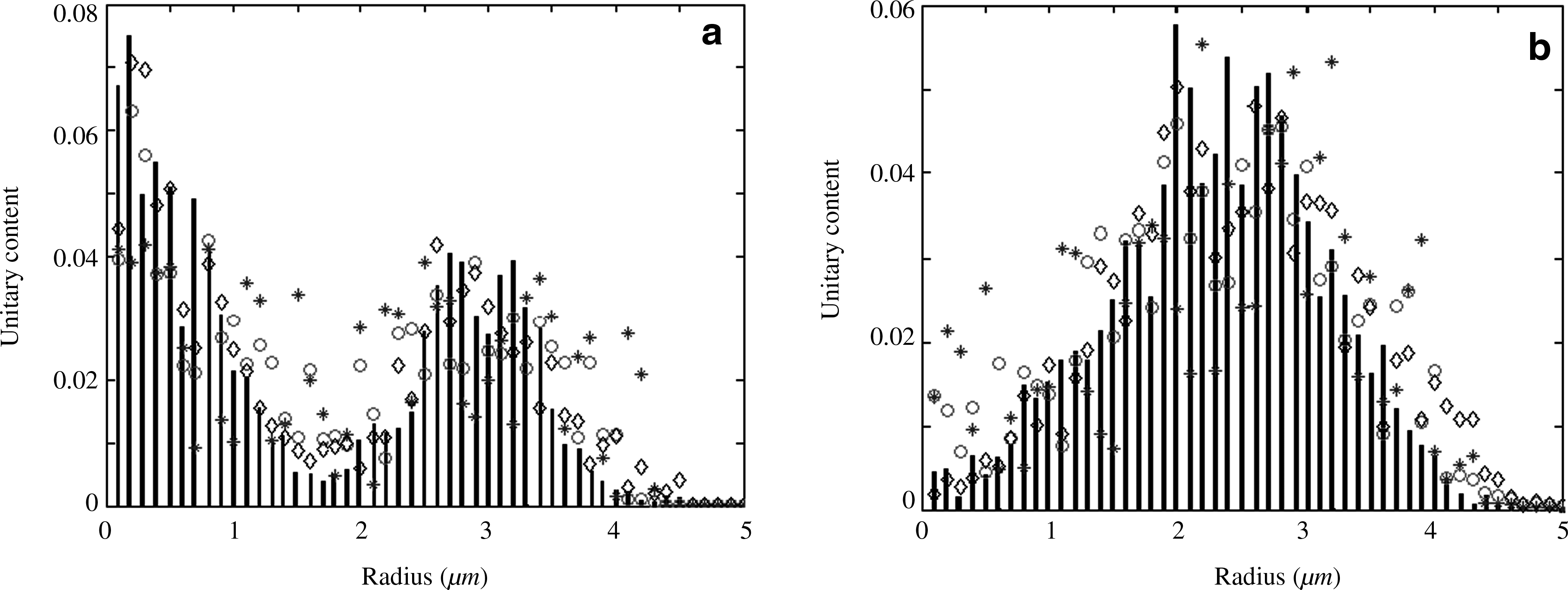
The size-distributions of polystyrene particles. Histograms: measured by using microscope; the asterisks: retrieved by using linear-regression; the rings: retrieved by using GA; the diamonds: retrieved by using AGA. The correlation coefficient between the asterisks and the histograms is
The setup used to measure τ(λ) is shown in Fig. 6. An Xe lamp can emit polychromatic light stably. The output light from the cell can be guided into a spectrograph (300–900 nm) by a fiber. First, the cell is filled with pure de-ionized water, and the output light (I0(λ)) is captured by using the spectrograph with 2000 times of sampling-average. Then, the particles are dispersed into the de-ionized water homogeneously, and output light (I1(λ)) is captured again by using the same spectrograph. Finally, substituting I0(λ) and I1(λ) into equation (1), the values of the τ(λ) can be got.
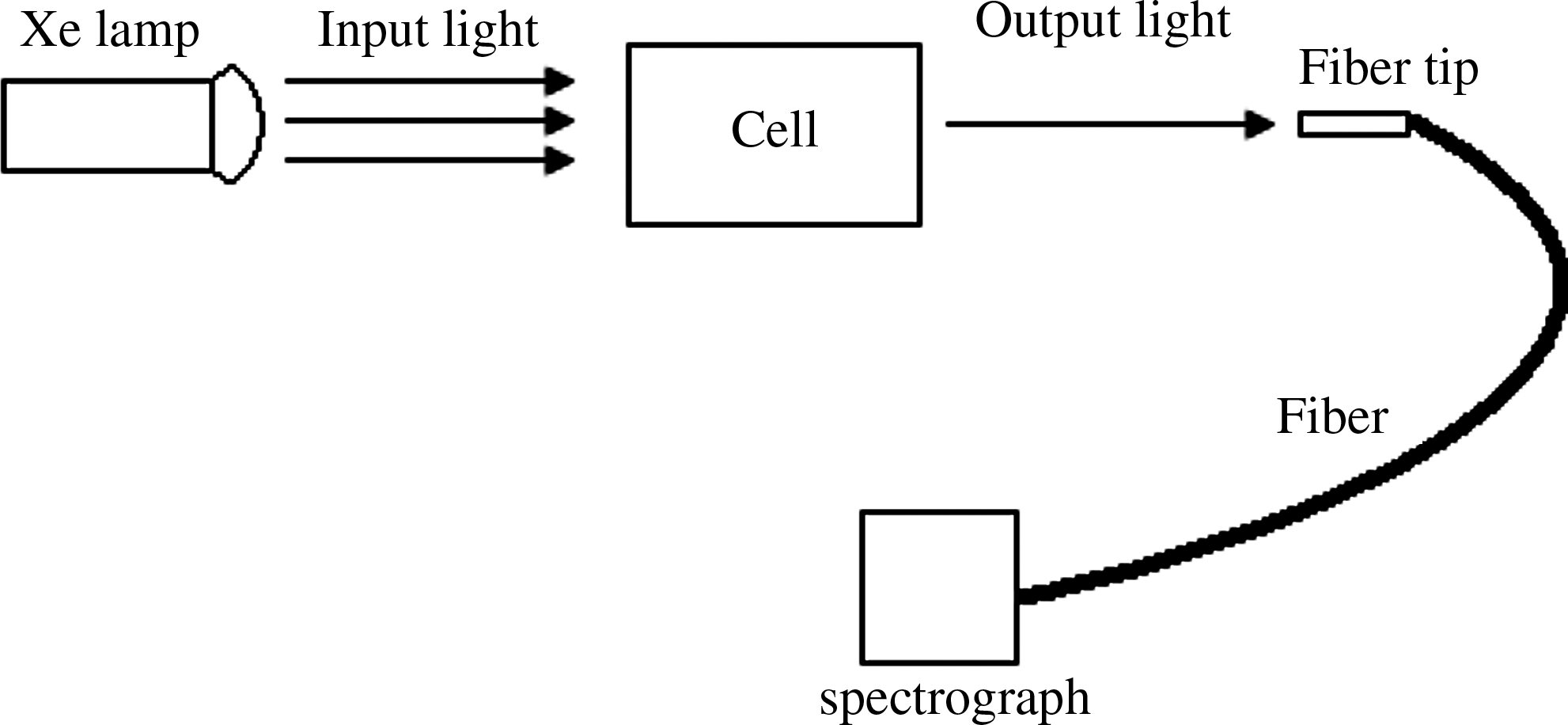
Setup used to measure the size-distribution.
Based on the τ(λ), the size-distributions are retrieved by using the LR, GA, and AGA respectively, with the results shown in Fig. 5. From Fig. 5, it can be seen that the results from the AGA are the best; the correlation coefficients between the retrieved size-distributions and the standard size-distributions exceed 0.9; the results from the GA, although they are worse than those from the AGA, are also acceptable; whereas the results from the LR are too bad to be accepted.
Conclusions
The stability and accuracy of retrieving the aerosol size-distribution by using LR, GA, and AGA are studied in detail. From the results of numeric simulation, it can be concluded that by using AGA the retrieval results are quite stable and accurate; by using the GA, the stability and accuracy are decreased mildly, but the results are still acceptable to some extent; by using the LR, the retrieval results are so unstable that the tiny errors of the τ(λ) could cause great errors of the retrieval results. This conclusion is further verified by the retrieval of the size distribution of the polystyrene particles in the water.
Footnotes
Acknowledgment
This research was supported by the National Natural Science Foundation of China (NSFC, No. 10875083).
Author Disclosure Statement
No competing financial interests exist.