Kinetics of Permanganate Consumption by Natural Oxidant Demand in Aquifer Solids

Introduction

I n situ chemical oxidation (ISCO) using permanganate ( \documentclass{aastex}\usepackage{amsbsy}\usepackage{amsfonts}\usepackage{amssymb}\usepackage{bm}\usepackage{mathrsfs}\usepackage{pifont}\usepackage{stmaryrd}\usepackage{textcomp}\usepackage{portland, xspace}\usepackage{amsmath, amsxtra}\pagestyle{empty}\DeclareMathSizes{10}{9}{7}{6}\begin{document} $${\rm MnO}_4^-$$ \end{document} ) can be very effective for treatment of chlorinated ethenes including perchloroethene, trichloroethene, and some aromatic hydrocarbons (naphthalene, phenanthrene, pyrene, and phenols) (Yan and Schwartz, 1999; Siegrist et al., 2001). When \documentclass{aastex}\usepackage{amsbsy}\usepackage{amsfonts}\usepackage{amssymb}\usepackage{bm}\usepackage{mathrsfs}\usepackage{pifont}\usepackage{stmaryrd}\usepackage{textcomp}\usepackage{portland, xspace}\usepackage{amsmath, amsxtra}\pagestyle{empty}\DeclareMathSizes{10}{9}{7}{6}\begin{document} $${\rm MnO}_4^-$$ \end{document} is injected into the subsurface, \documentclass{aastex}\usepackage{amsbsy}\usepackage{amsfonts}\usepackage{amssymb}\usepackage{bm}\usepackage{mathrsfs}\usepackage{pifont}\usepackage{stmaryrd}\usepackage{textcomp}\usepackage{portland, xspace}\usepackage{amsmath, amsxtra}\pagestyle{empty}\DeclareMathSizes{10}{9}{7}{6}\begin{document} $${\rm MnO}_4^-$$ \end{document} accepts three electrons and is subsequently reduced to MnO₂ solids (Siegrist et al., 2001). A portion of the electrons consumed are from oxidation of the target contaminant, and a portion are from the aquifer material including natural organic matter (NOM), reduced iron, manganese, and sulfur minerals (Yan and Schwartz, 1999; Siegrist et al., 2001; Mumford et al., 2005; Hønning et al., 2007; Urynowicz, 2008; Urynowicz et al., 2008). The amount of \documentclass{aastex}\usepackage{amsbsy}\usepackage{amsfonts}\usepackage{amssymb}\usepackage{bm}\usepackage{mathrsfs}\usepackage{pifont}\usepackage{stmaryrd}\usepackage{textcomp}\usepackage{portland, xspace}\usepackage{amsmath, amsxtra}\pagestyle{empty}\DeclareMathSizes{10}{9}{7}{6}\begin{document} $${\rm MnO}_4^-$$ \end{document} that reacts with nontarget chemicals is often referred to as natural oxidant demand (NOD) and can vary from <1% to over 99% of the total \documentclass{aastex}\usepackage{amsbsy}\usepackage{amsfonts}\usepackage{amssymb}\usepackage{bm}\usepackage{mathrsfs}\usepackage{pifont}\usepackage{stmaryrd}\usepackage{textcomp}\usepackage{portland, xspace}\usepackage{amsmath, amsxtra}\pagestyle{empty}\DeclareMathSizes{10}{9}{7}{6}\begin{document} $${\rm MnO}_4^-$$ \end{document} demand, depending on the contaminant concentration and aquifer characteristics. When NOD is high, then contaminant treatment efficiency may be less than desired due to nonproductive consumption of \documentclass{aastex}\usepackage{amsbsy}\usepackage{amsfonts}\usepackage{amssymb}\usepackage{bm}\usepackage{mathrsfs}\usepackage{pifont}\usepackage{stmaryrd}\usepackage{textcomp}\usepackage{portland, xspace}\usepackage{amsmath, amsxtra}\pagestyle{empty}\DeclareMathSizes{10}{9}{7}{6}\begin{document} $${\rm MnO}_4^-$$ \end{document} (Siegrist et al., 2001; Urynowicz, 2008).

The reaction between \documentclass{aastex}\usepackage{amsbsy}\usepackage{amsfonts}\usepackage{amssymb}\usepackage{bm}\usepackage{mathrsfs}\usepackage{pifont}\usepackage{stmaryrd}\usepackage{textcomp}\usepackage{portland, xspace}\usepackage{amsmath, amsxtra}\pagestyle{empty}\DeclareMathSizes{10}{9}{7}{6}\begin{document} $${\rm MnO}_4^-$$ \end{document} and NOD will depend on \documentclass{aastex}\usepackage{amsbsy}\usepackage{amsfonts}\usepackage{amssymb}\usepackage{bm}\usepackage{mathrsfs}\usepackage{pifont}\usepackage{stmaryrd}\usepackage{textcomp}\usepackage{portland, xspace}\usepackage{amsmath, amsxtra}\pagestyle{empty}\DeclareMathSizes{10}{9}{7}{6}\begin{document} $${\rm MnO}_4^-$$ \end{document} concentration and reaction time, as some fraction of the NOD may react slowly. Mumford et al. (2005) found that NOD exerted during short-term column experiments was much lower than that in long-term batch incubations. Even after 21 weeks incubation, the NOD in the soil was not completely oxidized and \documentclass{aastex}\usepackage{amsbsy}\usepackage{amsfonts}\usepackage{amssymb}\usepackage{bm}\usepackage{mathrsfs}\usepackage{pifont}\usepackage{stmaryrd}\usepackage{textcomp}\usepackage{portland, xspace}\usepackage{amsmath, amsxtra}\pagestyle{empty}\DeclareMathSizes{10}{9}{7}{6}\begin{document} $${\rm MnO}_4^-$$ \end{document} continued to be depleted. Several investigators (Yan and Schwartz, 1999; Siegrist et al., 2001; Mumford et al., 2005; Urynowicz et al., 2008) have reported that the measured NOD varies with the \documentclass{aastex}\usepackage{amsbsy}\usepackage{amsfonts}\usepackage{amssymb}\usepackage{bm}\usepackage{mathrsfs}\usepackage{pifont}\usepackage{stmaryrd}\usepackage{textcomp}\usepackage{portland, xspace}\usepackage{amsmath, amsxtra}\pagestyle{empty}\DeclareMathSizes{10}{9}{7}{6}\begin{document} $${\rm MnO}_4^-$$ \end{document} concentration and reaction time. Higher concentrations of \documentclass{aastex}\usepackage{amsbsy}\usepackage{amsfonts}\usepackage{amssymb}\usepackage{bm}\usepackage{mathrsfs}\usepackage{pifont}\usepackage{stmaryrd}\usepackage{textcomp}\usepackage{portland, xspace}\usepackage{amsmath, amsxtra}\pagestyle{empty}\DeclareMathSizes{10}{9}{7}{6}\begin{document} $${\rm MnO}_4^-$$ \end{document} commonly result in higher measured values of NOD (Siegrist, 2001; Hønning et al., 2007; Urynowicz et al., 2008). To reflect these observations, \documentclass{aastex}\usepackage{amsbsy}\usepackage{amsfonts}\usepackage{amssymb}\usepackage{bm}\usepackage{mathrsfs}\usepackage{pifont}\usepackage{stmaryrd}\usepackage{textcomp}\usepackage{portland, xspace}\usepackage{amsmath, amsxtra}\pagestyle{empty}\DeclareMathSizes{10}{9}{7}{6}\begin{document} $${\rm MnO}_4^-$$ \end{document} consumption is commonly modeled as a second order reaction between \documentclass{aastex}\usepackage{amsbsy}\usepackage{amsfonts}\usepackage{amssymb}\usepackage{bm}\usepackage{mathrsfs}\usepackage{pifont}\usepackage{stmaryrd}\usepackage{textcomp}\usepackage{portland, xspace}\usepackage{amsmath, amsxtra}\pagestyle{empty}\DeclareMathSizes{10}{9}{7}{6}\begin{document} $${\rm MnO}_4^-$$ \end{document} and NOD (Zhang and Schwartz, 2000; Urynowicz et al., 2008; Xu and Thomson, 2009).

More recent work has shown that NOD is composed of several components or fractions with varying reactivity (Mumford et al., 2005; Hønning et al., 2007; Urynowicz et al., 2008; Xu and Thomson, 2009). Ideally, NOD would be represented with a continuum of reaction rates where the less reactive fraction becomes progressively more important as the more reactive NOD fraction is depleted. However, studies by Urynowicz et al. (2008) and Xu and Thomson (2009) suggest that \documentclass{aastex}\usepackage{amsbsy}\usepackage{amsfonts}\usepackage{amssymb}\usepackage{bm}\usepackage{mathrsfs}\usepackage{pifont}\usepackage{stmaryrd}\usepackage{textcomp}\usepackage{portland, xspace}\usepackage{amsmath, amsxtra}\pagestyle{empty}\DeclareMathSizes{10}{9}{7}{6}\begin{document} $${\rm MnO}_4^-$$ \end{document} consumption by NOD can be reasonably well described by assuming that NOD is composed of disparate fast and slow fractions. In batch experiments conducted by Urynowicz et al. (2008), the fast NOD appeared to be consumed within about 48 h, followed by a slower depletion of \documentclass{aastex}\usepackage{amsbsy}\usepackage{amsfonts}\usepackage{amssymb}\usepackage{bm}\usepackage{mathrsfs}\usepackage{pifont}\usepackage{stmaryrd}\usepackage{textcomp}\usepackage{portland, xspace}\usepackage{amsmath, amsxtra}\pagestyle{empty}\DeclareMathSizes{10}{9}{7}{6}\begin{document} $${\rm MnO}_4^-$$ \end{document} at rates of 0.024 to 0.13 day⁻¹, depending on \documentclass{aastex}\usepackage{amsbsy}\usepackage{amsfonts}\usepackage{amssymb}\usepackage{bm}\usepackage{mathrsfs}\usepackage{pifont}\usepackage{stmaryrd}\usepackage{textcomp}\usepackage{portland, xspace}\usepackage{amsmath, amsxtra}\pagestyle{empty}\DeclareMathSizes{10}{9}{7}{6}\begin{document} $${\rm MnO}_4^-$$ \end{document} dose. Xu and Thomson (2009) found that a fraction of NOD was depleted in a few hours followed by much slower degradation, where the slow NOD reaction rate varied from 0.014 to 0.72 L/mmol-day with a median value of 0.077 L/mmol-day, in batch experiments.

Objective and Approach

The performance of ISCO systems can potentially be improved by using numerical models to simulate ISCO with \documentclass{aastex}\usepackage{amsbsy}\usepackage{amsfonts}\usepackage{amssymb}\usepackage{bm}\usepackage{mathrsfs}\usepackage{pifont}\usepackage{stmaryrd}\usepackage{textcomp}\usepackage{portland, xspace}\usepackage{amsmath, amsxtra}\pagestyle{empty}\DeclareMathSizes{10}{9}{7}{6}\begin{document} $${\rm MnO}_4^-$$ \end{document} under realistic conditions using spatially heterogeneous, three-dimensional flow, transport, and chemical reaction models. However, simulation of ISCO with \documentclass{aastex}\usepackage{amsbsy}\usepackage{amsfonts}\usepackage{amssymb}\usepackage{bm}\usepackage{mathrsfs}\usepackage{pifont}\usepackage{stmaryrd}\usepackage{textcomp}\usepackage{portland, xspace}\usepackage{amsmath, amsxtra}\pagestyle{empty}\DeclareMathSizes{10}{9}{7}{6}\begin{document} $${\rm MnO}_4^-$$ \end{document} requires constitutive relationships that accurately represent the kinetics of \documentclass{aastex}\usepackage{amsbsy}\usepackage{amsfonts}\usepackage{amssymb}\usepackage{bm}\usepackage{mathrsfs}\usepackage{pifont}\usepackage{stmaryrd}\usepackage{textcomp}\usepackage{portland, xspace}\usepackage{amsmath, amsxtra}\pagestyle{empty}\DeclareMathSizes{10}{9}{7}{6}\begin{document} $${\rm MnO}_4^-$$ \end{document} consumption by NOD for a range of conditions. Ideally, these kinetic models could be applied without imposing an excessive computational burden, using parameters estimated from standard NOD test protocols.

In the work presented here, six different kinetic models were fit to data from batch NOD tests on 50 different aquifer samples with varying \documentclass{aastex}\usepackage{amsbsy}\usepackage{amsfonts}\usepackage{amssymb}\usepackage{bm}\usepackage{mathrsfs}\usepackage{pifont}\usepackage{stmaryrd}\usepackage{textcomp}\usepackage{portland, xspace}\usepackage{amsmath, amsxtra}\pagestyle{empty}\DeclareMathSizes{10}{9}{7}{6}\begin{document} $${\rm MnO}_4^-$$ \end{document} concentrations and/or aquifer solid to water ratios following ASTM D 7262-07 (2007). The six models evaluated are summarized in Table 1. Subroutines were developed within MS Excel for each model and applied to automatically estimate model parameters for each aquifer sample. Results of this work were used to identify the models that best fit the experimental results and to generate a database of parameters which can be used in future modeling studies.

The models examined in this work included simple zero- and first-order single parameter models (1, 2, and 3) and second-order models incorporating the effects of oxidant concentration and NOD concentration (4, 5, and 6). For Models 5 and 6, NOD was assumed to be composed of slowly reacting and fast/instantaneously reacting components. This work aimed at developing relatively simple models that could accurately represent reaction kinetics without imposing an excessive computational burden and, therefore, only terms that could be estimated from the standard ASTM test protocol were used in the simulations.

Model evaluation

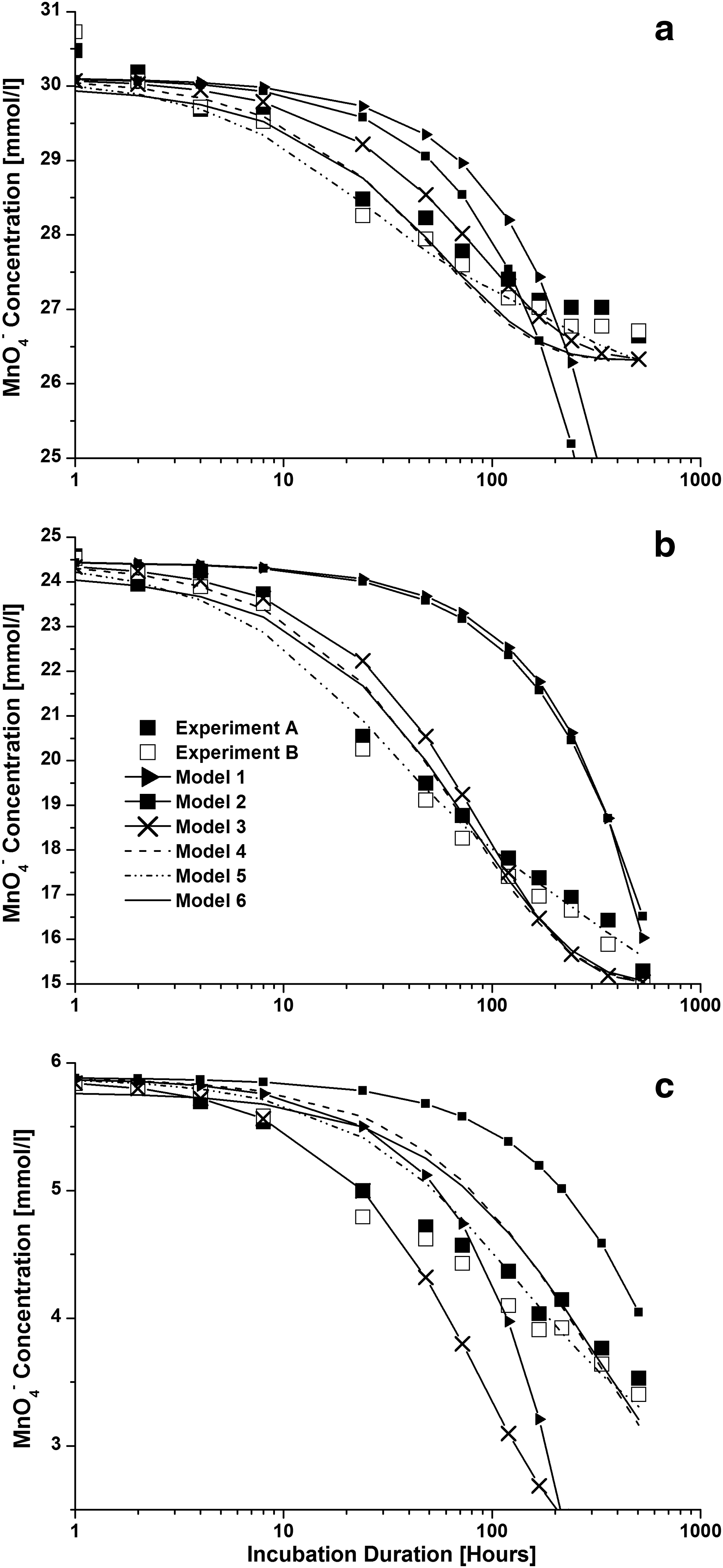
Each of the six models were fit to the NOD experimental results for each of the 50 aquifer solids. Figure 1 shows typical results for a single aquifer solid (YT-YS2). Aquifer sample YT-YS2 was tested in duplicate (Experiment A and Experiment B) with three experimental treatments ( \documentclass{aastex}\usepackage{amsbsy}\usepackage{amsfonts}\usepackage{amssymb}\usepackage{bm}\usepackage{mathrsfs}\usepackage{pifont}\usepackage{stmaryrd}\usepackage{textcomp}\usepackage{portland, xspace}\usepackage{amsmath, amsxtra}\pagestyle{empty}\DeclareMathSizes{10}{9}{7}{6}\begin{document} $${\rm MnO}_4^- = 30.1$$ \end{document} , 24.5, or 5.9 mM; solid:water ratio=0.38 or 0.95 g aquifer solids per mL water) over 22 days, thereby resulting in a total of 78 concentration measurements. Over the 22-day experimental period, \documentclass{aastex}\usepackage{amsbsy}\usepackage{amsfonts}\usepackage{amssymb}\usepackage{bm}\usepackage{mathrsfs}\usepackage{pifont}\usepackage{stmaryrd}\usepackage{textcomp}\usepackage{portland, xspace}\usepackage{amsmath, amsxtra}\pagestyle{empty}\DeclareMathSizes{10}{9}{7}{6}\begin{document} $${\rm MnO}_4^-$$ \end{document} concentration declined by up to 9 mM as the oxidant was consumed by NOD. The difference in \documentclass{aastex}\usepackage{amsbsy}\usepackage{amsfonts}\usepackage{amssymb}\usepackage{bm}\usepackage{mathrsfs}\usepackage{pifont}\usepackage{stmaryrd}\usepackage{textcomp}\usepackage{portland, xspace}\usepackage{amsmath, amsxtra}\pagestyle{empty}\DeclareMathSizes{10}{9}{7}{6}\begin{document} $${\rm MnO}_4^-$$ \end{document} consumption between the three different treatments is presumably due to differences in initial \documentclass{aastex}\usepackage{amsbsy}\usepackage{amsfonts}\usepackage{amssymb}\usepackage{bm}\usepackage{mathrsfs}\usepackage{pifont}\usepackage{stmaryrd}\usepackage{textcomp}\usepackage{portland, xspace}\usepackage{amsmath, amsxtra}\pagestyle{empty}\DeclareMathSizes{10}{9}{7}{6}\begin{document} $${\rm MnO}_4^-$$ \end{document} concentration and aquifer solids to water ratio.

OPEN IN VIEWER

FIG. 1.

Comparison of simulated and observed \documentclass{aastex}\usepackage{amsbsy}\usepackage{amsfonts}\usepackage{amssymb}\usepackage{bm}\usepackage{mathrsfs}\usepackage{pifont}\usepackage{stmaryrd}\usepackage{textcomp}\usepackage{portland, xspace}\usepackage{amsmath, amsxtra}\pagestyle{empty}\DeclareMathSizes{10}{9}{7}{6}\begin{document} $${\rm MnO}_4^-$$ \end{document} concentrations for aquifer sample YT-YS2 with (a) 30.1 mmol/L initial \documentclass{aastex}\usepackage{amsbsy}\usepackage{amsfonts}\usepackage{amssymb}\usepackage{bm}\usepackage{mathrsfs}\usepackage{pifont}\usepackage{stmaryrd}\usepackage{textcomp}\usepackage{portland, xspace}\usepackage{amsmath, amsxtra}\pagestyle{empty}\DeclareMathSizes{10}{9}{7}{6}\begin{document} $${\rm MnO}_4^-$$ \end{document} concentration and 0.38 g solids per mL water; (b) 24.5 mmol/L \documentclass{aastex}\usepackage{amsbsy}\usepackage{amsfonts}\usepackage{amssymb}\usepackage{bm}\usepackage{mathrsfs}\usepackage{pifont}\usepackage{stmaryrd}\usepackage{textcomp}\usepackage{portland, xspace}\usepackage{amsmath, amsxtra}\pagestyle{empty}\DeclareMathSizes{10}{9}{7}{6}\begin{document} $${\rm MnO}_4^-$$ \end{document} and 0.38 g solids/mL; and (c) 5.9 mmol/L \documentclass{aastex}\usepackage{amsbsy}\usepackage{amsfonts}\usepackage{amssymb}\usepackage{bm}\usepackage{mathrsfs}\usepackage{pifont}\usepackage{stmaryrd}\usepackage{textcomp}\usepackage{portland, xspace}\usepackage{amsmath, amsxtra}\pagestyle{empty}\DeclareMathSizes{10}{9}{7}{6}\begin{document} $${\rm MnO}_4^-$$ \end{document} and 0.95 g solids/mL. \documentclass{aastex}\usepackage{amsbsy}\usepackage{amsfonts}\usepackage{amssymb}\usepackage{bm}\usepackage{mathrsfs}\usepackage{pifont}\usepackage{stmaryrd}\usepackage{textcomp}\usepackage{portland, xspace}\usepackage{amsmath, amsxtra}\pagestyle{empty}\DeclareMathSizes{10}{9}{7}{6}\begin{document} $${\rm MnO}_4^-$$ \end{document} , permanganate.

The lines shown in Fig. 1 are simulation results generated by using the single set of coefficients for each model. The model coefficients were determined by (a) calculating the error between simulated and observed concentration; (b) calculating the RMSE for the entire YT-YS2 data set; and (c) searching for the model coefficients that minimized the RMSE. Models 1 and 2 do not follow the overall trends in the data and provide a poor match to the experimental results for all three treatments. Model 3 provides a reasonably good fit to the two higher concentration experiments (Fig. 1a, b), but significantly underestimates the \documentclass{aastex}\usepackage{amsbsy}\usepackage{amsfonts}\usepackage{amssymb}\usepackage{bm}\usepackage{mathrsfs}\usepackage{pifont}\usepackage{stmaryrd}\usepackage{textcomp}\usepackage{portland, xspace}\usepackage{amsmath, amsxtra}\pagestyle{empty}\DeclareMathSizes{10}{9}{7}{6}\begin{document} $${\rm MnO}_4^-$$ \end{document} concentrations during much of the low concentration experiment (Fig. 1c). In contrast, Models 4, 5, and 6 provide a reasonably good match with the general trends in \documentclass{aastex}\usepackage{amsbsy}\usepackage{amsfonts}\usepackage{amssymb}\usepackage{bm}\usepackage{mathrsfs}\usepackage{pifont}\usepackage{stmaryrd}\usepackage{textcomp}\usepackage{portland, xspace}\usepackage{amsmath, amsxtra}\pagestyle{empty}\DeclareMathSizes{10}{9}{7}{6}\begin{document} $${\rm MnO}_4^-$$ \end{document} concentration versus time for all three treatments.

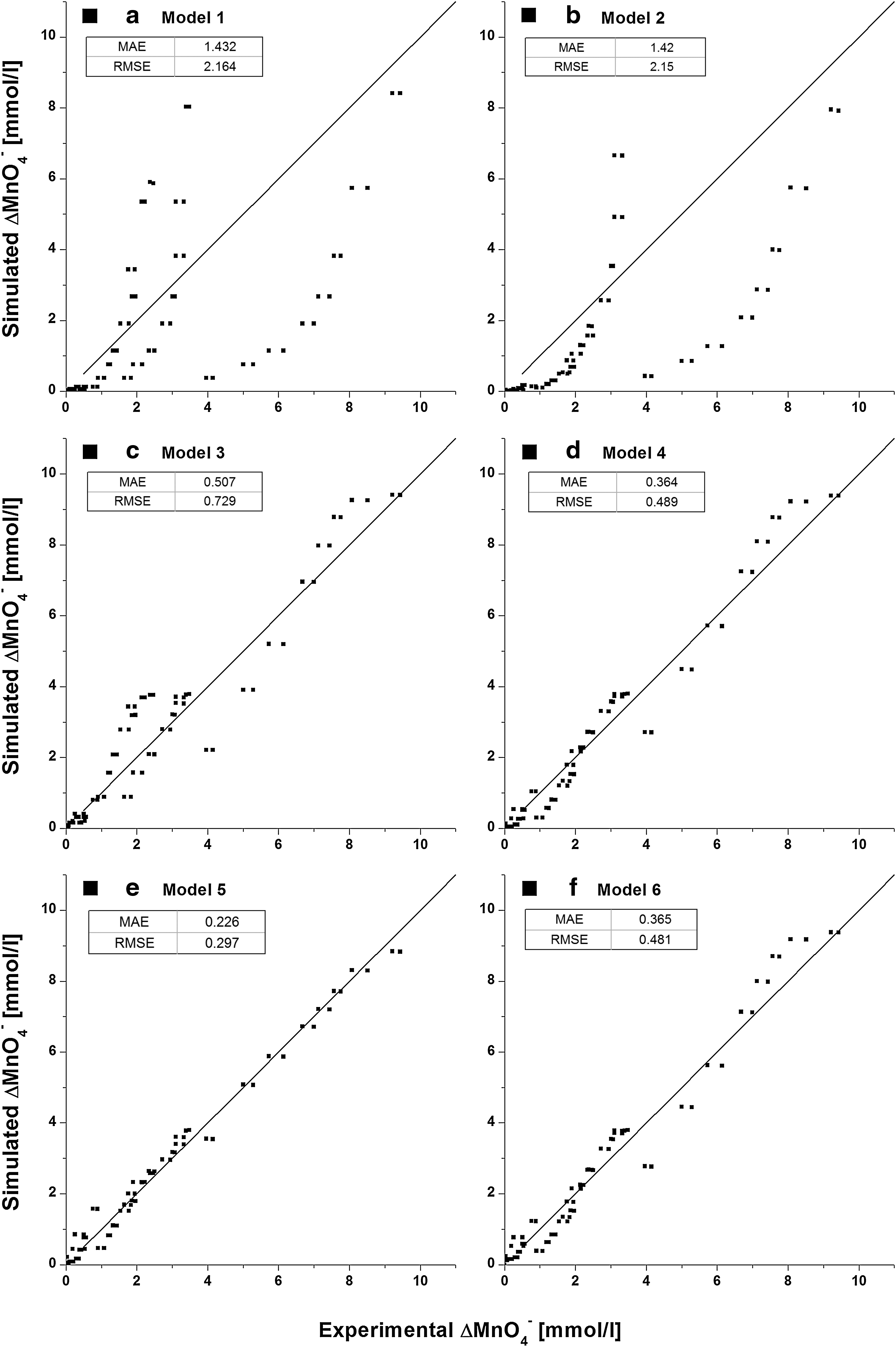
Data from Fig. 1 are replotted in Fig. 2 to better illustrate the performance of the different models. For every experimental measurement, the change in \documentclass{aastex}\usepackage{amsbsy}\usepackage{amsfonts}\usepackage{amssymb}\usepackage{bm}\usepackage{mathrsfs}\usepackage{pifont}\usepackage{stmaryrd}\usepackage{textcomp}\usepackage{portland, xspace}\usepackage{amsmath, amsxtra}\pagestyle{empty}\DeclareMathSizes{10}{9}{7}{6}\begin{document} $${\rm MnO}_4^-$$ \end{document} concentration ( \documentclass{aastex}\usepackage{amsbsy}\usepackage{amsfonts}\usepackage{amssymb}\usepackage{bm}\usepackage{mathrsfs}\usepackage{pifont}\usepackage{stmaryrd}\usepackage{textcomp}\usepackage{portland, xspace}\usepackage{amsmath, amsxtra}\pagestyle{empty}\DeclareMathSizes{10}{9}{7}{6}\begin{document} $$\Delta {\rm MnO}_4^-$$ \end{document} ) was computed as the difference between the initial concentration and the measured concentration and compared with the simulated \documentclass{aastex}\usepackage{amsbsy}\usepackage{amsfonts}\usepackage{amssymb}\usepackage{bm}\usepackage{mathrsfs}\usepackage{pifont}\usepackage{stmaryrd}\usepackage{textcomp}\usepackage{portland, xspace}\usepackage{amsmath, amsxtra}\pagestyle{empty}\DeclareMathSizes{10}{9}{7}{6}\begin{document} $$\Delta {\rm MnO}_4^-$$ \end{document} for each model. Figure 2 shows a comparison of simulated and experimental \documentclass{aastex}\usepackage{amsbsy}\usepackage{amsfonts}\usepackage{amssymb}\usepackage{bm}\usepackage{mathrsfs}\usepackage{pifont}\usepackage{stmaryrd}\usepackage{textcomp}\usepackage{portland, xspace}\usepackage{amsmath, amsxtra}\pagestyle{empty}\DeclareMathSizes{10}{9}{7}{6}\begin{document} $$\Delta {\rm MnO}_4^-$$ \end{document} for all 78 measurements made with the YT-YS2 aquifer solids. Ideally, all the data would plot along the solid 45-degree line, thus indicating a perfect match between simulated and observed values. For Models 1 and 2 (Fig. 2a, b), the data points show clear trends above and below the 1:1 line, thus indicating a very poor match with the experimental results. For Model 3 (Fig. 2c), the data generally plot along the 1:1 line, thus indicating a relatively good match to the data. However, there are areas where groups of points are clustered above or below the 1:1 line, thus indicating some underlying trend that is not captured by the model. In contrast, the data points for Models 4, 5, and 6 plot along the 45-degree line with no obvious trends in \documentclass{aastex}\usepackage{amsbsy}\usepackage{amsfonts}\usepackage{amssymb}\usepackage{bm}\usepackage{mathrsfs}\usepackage{pifont}\usepackage{stmaryrd}\usepackage{textcomp}\usepackage{portland, xspace}\usepackage{amsmath, amsxtra}\pagestyle{empty}\DeclareMathSizes{10}{9}{7}{6}\begin{document} $$\Delta {\rm MnO}_4^-$$ \end{document} . Model 5 with four calibration parameters provides the lowest mean absolute error (MAE) and RMSE, indicating that it provided the best fit to the YT-YS2 experimental results. However, Model 6, with three calibration parameters, provided a relatively good fit to the experimental data with both MAE and RMSE <5% of the maximum \documentclass{aastex}\usepackage{amsbsy}\usepackage{amsfonts}\usepackage{amssymb}\usepackage{bm}\usepackage{mathrsfs}\usepackage{pifont}\usepackage{stmaryrd}\usepackage{textcomp}\usepackage{portland, xspace}\usepackage{amsmath, amsxtra}\pagestyle{empty}\DeclareMathSizes{10}{9}{7}{6}\begin{document} $$\Delta {\rm MnO}_4^-$$ \end{document} .

OPEN IN VIEWER

FIG. 2.

Simulated versus observed \documentclass{aastex}\usepackage{amsbsy}\usepackage{amsfonts}\usepackage{amssymb}\usepackage{bm}\usepackage{mathrsfs}\usepackage{pifont}\usepackage{stmaryrd}\usepackage{textcomp}\usepackage{portland, xspace}\usepackage{amsmath, amsxtra}\pagestyle{empty}\DeclareMathSizes{10}{9}{7}{6}\begin{document} $$\Delta {\rm MnO}_4^-$$ \end{document} for all treatments of YT-YS2: (a) Model 1, (b) Model 2, (c) Model 3, (d) Model 4, (e) Model 5, and (f) Model 6. Solid line represents a perfect match between simulated and observed \documentclass{aastex}\usepackage{amsbsy}\usepackage{amsfonts}\usepackage{amssymb}\usepackage{bm}\usepackage{mathrsfs}\usepackage{pifont}\usepackage{stmaryrd}\usepackage{textcomp}\usepackage{portland, xspace}\usepackage{amsmath, amsxtra}\pagestyle{empty}\DeclareMathSizes{10}{9}{7}{6}\begin{document} $$\Delta {\rm MnO}_4^-$$ \end{document} .

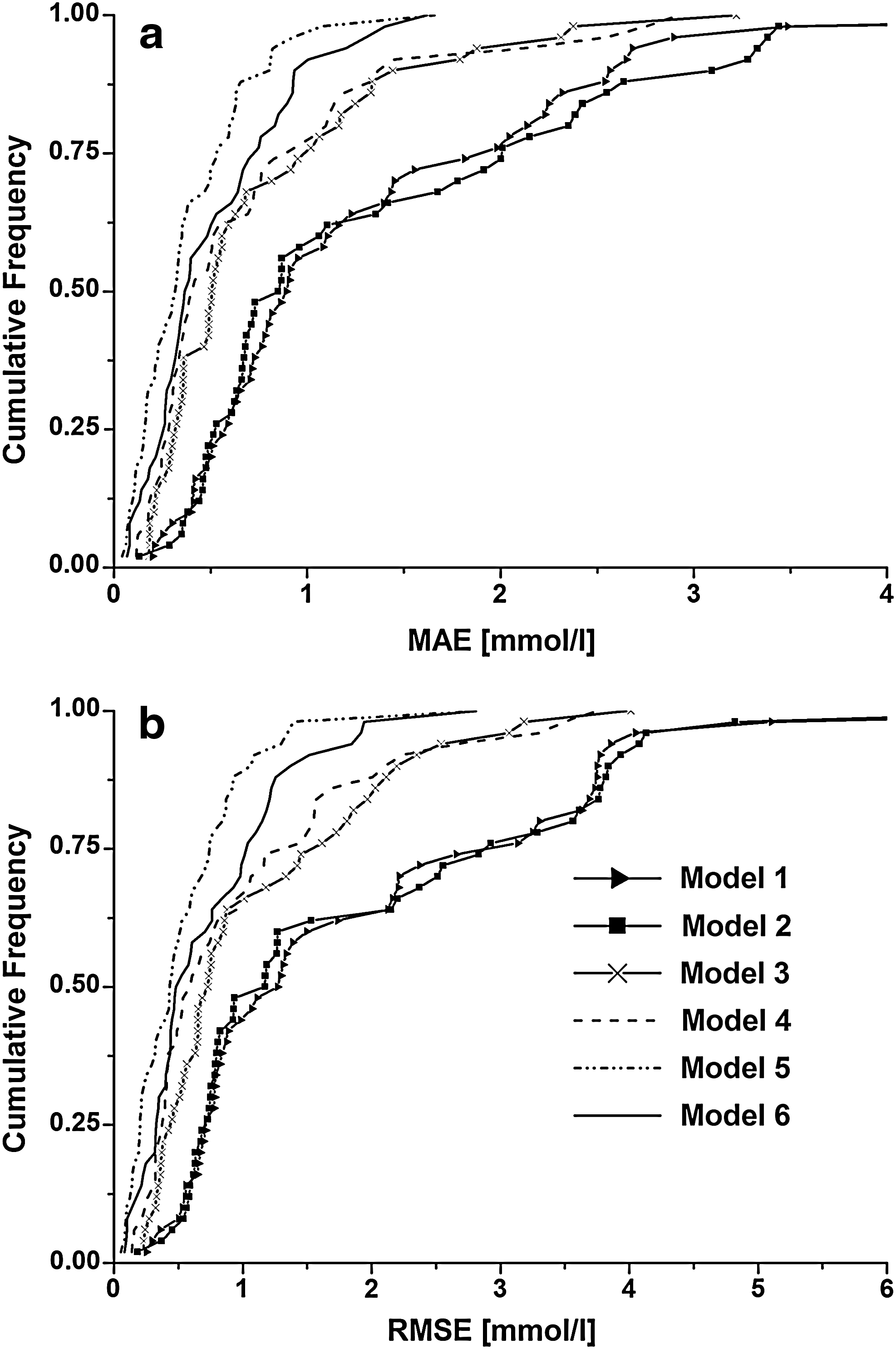
Figure 3 shows cumulative frequency distributions for the MAE and RMSE for each model for all 50 aquifer solid samples. Model 5 (4 parameters), Model 6 (3 parameters), and Model 4 (2 parameters) provide relatively good fits (low MAE and RMSE) to the experimental data for more than 50% of the aquifer samples. However, for the worst 10%–20% of the samples (highest MAE and RMSE), the performance of Models 5 and 6 is substantially better than that of Model 4.

OPEN IN VIEWER

FIG. 3.

Cumulative frequency distributions of (a) mean absolute error (MAE) and (b) root-mean-square error (RMSE) for Models 1–6 using NOD data from 50 aquifer solids. NOD, natural oxidant demand.

To provide an overall estimate of model performance, the data on model fit to all 50 aquifer solids were pooled together (2894 \documentclass{aastex}\usepackage{amsbsy}\usepackage{amsfonts}\usepackage{amssymb}\usepackage{bm}\usepackage{mathrsfs}\usepackage{pifont}\usepackage{stmaryrd}\usepackage{textcomp}\usepackage{portland, xspace}\usepackage{amsmath, amsxtra}\pagestyle{empty}\DeclareMathSizes{10}{9}{7}{6}\begin{document} $${\rm MnO}_4^-$$ \end{document} measurements) and used to compute the global MAE and RMSE (Table 2). Consistent with the previous discussion, Model 5 provided the best fit to the data (lowest MAE and RMSE), followed by Model 6, then Model 4, then Model 3. Models 1 and 2 provided a poor fit to the experimental results. A Kruskal–Wallis nonparametric test was conducted to evaluate whether the performance of Model 6 was significantly different from that of Model 5 based on the distribution of absolute error (Ott and Longnecker, 2001). Using the pooled data from all 50 samples, the difference in the performance of Model 5 and 6 was significant at the 0.001 level. However, when applied to individual aquifer solids, there was no significant difference between Models 5 and 6 for 39 of the 50 samples (78%). This indicates that for the total data set from the 50 aquifer solids, Model 5 is superior to Model 6. However for many individual aquifer solid samples, the difference is not significant.

OPEN IN VIEWER

Table 2.

Mean Absolute Error and Root-Mean-Square Error for Models 1–6 Using Pooled Data from 50 Aquifer Solids

Model	# of parameters	MAE (mmol/L)	RMSE (mmol/L)
1	1	1.31	2.40
2	1	1.36	2.38
3	2	0.81	1.46
4	2	0.70	1.22
5	4	0.46	0.80
6	3	0.58	0.98

MAE, mean absolute error; RMSE, root-mean-square error.

NOD parameter estimates

Parameter estimates and error statistics for Models 1 to 6 for the 50 aquifer solids are provided in Supplementary Tables S3 and S4. For Models 5 and 6, we report total NOD (NOD_T) and the fraction fast or instantaneous (f) to simplify comparison between the different models and to be consistent with previous studies. NOD_S=NOD_T (1 − f) and NOD_F and NOD_I=NOD_T × f. In most cases, parameter values were not normally or log normally distributed at the 0.05 level based on the Shapiro–Wilk test (Shapiro and Wilk, 1965). To provide a better representation of the parameter distributions, cumulative frequency plots for each of the Model 5 and 6 parameters are shown in Fig. 4. The 10, 25, 50, 75, and 90 percentile values for every model parameter are summarized in Table 3.

OPEN IN VIEWER

FIG. 4.

Cumulative frequency distributions for Models 5 and 6: kinetic parameters generated using NOD data from 50 aquifer solids.

OPEN IN VIEWER

Table 3.

Statistical Characteristics of Kinetic Parameter Distributions for Models 1–6 Generated Using Natural Oxidant Demand Data from 50 Aquifer Solids

			Percentile
Model	Parameter	Unit	10%	25%	50%	75%	90%
1	k0	mmol/L-day	0.055	0.074	0.521	1.170	2.746
2	k1M	1/day	0.010	0.015	0.035	0.077	0.290
3	NODT	mmol/g	0.001	0.002	0.027	0.069	0.158
	k1N	1/day	0.083	0.131	0.275	0.592	2.306
4	NODT	mmol/g	0.001	0.002	0.027	0.069	0.158
	k2	L/mmol-day	0.009	0.014	0.030	0.062	0.202
5	NODT	mmol/g	0.002	0.002	0.037	0.114	0.172
	Fraction instantaneous	–	0.087	0.181	0.248	0.424	0.553
	k2F	L/mmol-day	0.053	0.143	0.944	6.329	8.245
	K2S	L/mmol-day	0.001	0.002	0.006	0.017	0.028
6	NODT	mmol/g	0.002	0.002	0.028	0.070	0.158
	Fraction instantaneous	–	0.028	0.046	0.126	0.208	0.361
	k2S	L/mmol-day	0.003	0.008	0.018	0.036	0.395

Previous studies have reported large variations in the total amount of NOD. However, there is much less information on the fraction of fast/instantaneous NOD and reaction rate coefficients. In the 50 samples examined in this study, large variations in each of the parameters were observed, thus reflecting the wide variations in both the amount and reactivity of NOD in natural aquifer solids. Total NOD varied from 0.0013 to 0.95 mmol/g (equivalent to 0.2 to 150 g KMnO₄/kg), similar to previously reported ranges (Siegrist et al., 2001; Mumford et al., 2005; Hønning et al., 2007; Urynowicz, 2008; Xu and Thomson, 2009). The fraction fast/instantaneous varied from 1% to 67% with a median of 13%. The search procedure had a constraint that fraction fast/instantaneous ≥1%. However, this constraint only influenced one out of the 50 samples. For Model 5, fast reaction rates varied from 0.02 to over 10 L/mmol-day, whereas the slow reaction rates were typically 1 to 2 orders of magnitude lower. Model 6 reaction rates were typically intermediate between the Model 5 fast and slow rates.

Some practitioners estimate the aquifer NOD based on the amount of \documentclass{aastex}\usepackage{amsbsy}\usepackage{amsfonts}\usepackage{amssymb}\usepackage{bm}\usepackage{mathrsfs}\usepackage{pifont}\usepackage{stmaryrd}\usepackage{textcomp}\usepackage{portland, xspace}\usepackage{amsmath, amsxtra}\pagestyle{empty}\DeclareMathSizes{10}{9}{7}{6}\begin{document} $${\rm MnO}_4^-$$ \end{document} consumed over 48 h as a screening test for potential ISCO sites (ASTM D 7262-07). Figure 5 shows the ratio of the best fit value of total NOD for Models 5 and 6 to the 48-h value. This ratio varied widely, thus indicating that there is a very poor correlation between the best fit values of Total NOD to the 48-h NOD. This indicates that 48-h test results should not be used to estimate the amount of \documentclass{aastex}\usepackage{amsbsy}\usepackage{amsfonts}\usepackage{amssymb}\usepackage{bm}\usepackage{mathrsfs}\usepackage{pifont}\usepackage{stmaryrd}\usepackage{textcomp}\usepackage{portland, xspace}\usepackage{amsmath, amsxtra}\pagestyle{empty}\DeclareMathSizes{10}{9}{7}{6}\begin{document} $${\rm MnO}_4^-$$ \end{document} that may be consumed during extended incubation periods and should not be used to simulate \documentclass{aastex}\usepackage{amsbsy}\usepackage{amsfonts}\usepackage{amssymb}\usepackage{bm}\usepackage{mathrsfs}\usepackage{pifont}\usepackage{stmaryrd}\usepackage{textcomp}\usepackage{portland, xspace}\usepackage{amsmath, amsxtra}\pagestyle{empty}\DeclareMathSizes{10}{9}{7}{6}\begin{document} $${\rm MnO}_4^-$$ \end{document} consumption in transport models.

OPEN IN VIEWER

FIG. 5.

Cumulative frequency distributions showing ratio of best fit total NOD to 48-h NOD for Models 5 and 6 using NOD data from 50 aquifer solids.

Discussion

Some remediation practitioners estimate the amount of \documentclass{aastex}\usepackage{amsbsy}\usepackage{amsfonts}\usepackage{amssymb}\usepackage{bm}\usepackage{mathrsfs}\usepackage{pifont}\usepackage{stmaryrd}\usepackage{textcomp}\usepackage{portland, xspace}\usepackage{amsmath, amsxtra}\pagestyle{empty}\DeclareMathSizes{10}{9}{7}{6}\begin{document} $${\rm MnO}_4^-$$ \end{document} required for ISCO based on a few short-term NOD measurements. Once injected, the \documentclass{aastex}\usepackage{amsbsy}\usepackage{amsfonts}\usepackage{amssymb}\usepackage{bm}\usepackage{mathrsfs}\usepackage{pifont}\usepackage{stmaryrd}\usepackage{textcomp}\usepackage{portland, xspace}\usepackage{amsmath, amsxtra}\pagestyle{empty}\DeclareMathSizes{10}{9}{7}{6}\begin{document} $${\rm MnO}_4^-$$ \end{document} concentration will vary in time and space due to advection, dispersion, and consumption by the contaminant and NOD. Previous studies have shown that \documentclass{aastex}\usepackage{amsbsy}\usepackage{amsfonts}\usepackage{amssymb}\usepackage{bm}\usepackage{mathrsfs}\usepackage{pifont}\usepackage{stmaryrd}\usepackage{textcomp}\usepackage{portland, xspace}\usepackage{amsmath, amsxtra}\pagestyle{empty}\DeclareMathSizes{10}{9}{7}{6}\begin{document} $${\rm MnO}_4^-$$ \end{document} consumption varies with time, that higher \documentclass{aastex}\usepackage{amsbsy}\usepackage{amsfonts}\usepackage{amssymb}\usepackage{bm}\usepackage{mathrsfs}\usepackage{pifont}\usepackage{stmaryrd}\usepackage{textcomp}\usepackage{portland, xspace}\usepackage{amsmath, amsxtra}\pagestyle{empty}\DeclareMathSizes{10}{9}{7}{6}\begin{document} $${\rm MnO}_4^-$$ \end{document} concentrations often result in greater demand, and that NOD may be composed of several components or fractions with varying reactivity (Siegrist, 2001; Mumford et al., 2005; Hønning et al., 2007; Urynowicz et al., 2008; Xu and Thomson, 2009). Given this previous work, there is no simple way to estimate the required injection concentration and volume from a few simple measurements. To reduce remediation system costs and improve performance, a simple, easy-to-implement approach is needed for estimating \documentclass{aastex}\usepackage{amsbsy}\usepackage{amsfonts}\usepackage{amssymb}\usepackage{bm}\usepackage{mathrsfs}\usepackage{pifont}\usepackage{stmaryrd}\usepackage{textcomp}\usepackage{portland, xspace}\usepackage{amsmath, amsxtra}\pagestyle{empty}\DeclareMathSizes{10}{9}{7}{6}\begin{document} $${\rm MnO}_4^-$$ \end{document} distribution and longevity.

In this work, a simple procedure was developed and applied to estimate NOD kinetic parameters for six different models for 50 different samples of aquifer material. Consistent with previous work (Urynowicz, 2008; Xu and Thomson, 2009), simulation of \documentclass{aastex}\usepackage{amsbsy}\usepackage{amsfonts}\usepackage{amssymb}\usepackage{bm}\usepackage{mathrsfs}\usepackage{pifont}\usepackage{stmaryrd}\usepackage{textcomp}\usepackage{portland, xspace}\usepackage{amsmath, amsxtra}\pagestyle{empty}\DeclareMathSizes{10}{9}{7}{6}\begin{document} $${\rm MnO}_4^-$$ \end{document} consumption as a second-order reaction with separate fast and slow NOD fractions provided the best fit to the experimental data. For the 50 samples examined in this study, the median half life (T_½) for NOD_F was 0.02 days (range=10⁻⁴ to 2 days), and median T_½ for NOD_S was 9.4 days (range=10⁻² to 84 days). These results indicate that (a) the fast NOD fraction will be rapidly consumed; and (b) once the fast fraction is depleted, remaining \documentclass{aastex}\usepackage{amsbsy}\usepackage{amsfonts}\usepackage{amssymb}\usepackage{bm}\usepackage{mathrsfs}\usepackage{pifont}\usepackage{stmaryrd}\usepackage{textcomp}\usepackage{portland, xspace}\usepackage{amsmath, amsxtra}\pagestyle{empty}\DeclareMathSizes{10}{9}{7}{6}\begin{document} $${\rm MnO}_4^-$$ \end{document} may persist for weeks to months, diffusing into lower permeability zones where contaminants may reside. However, accurate simulation of \documentclass{aastex}\usepackage{amsbsy}\usepackage{amsfonts}\usepackage{amssymb}\usepackage{bm}\usepackage{mathrsfs}\usepackage{pifont}\usepackage{stmaryrd}\usepackage{textcomp}\usepackage{portland, xspace}\usepackage{amsmath, amsxtra}\pagestyle{empty}\DeclareMathSizes{10}{9}{7}{6}\begin{document} $${\rm MnO}_4^-$$ \end{document} consumption by the fast fraction (Model 5) will require very short time steps with a proportionate increase in computer run times. In contrast, if the fast fraction is assumed to react instantaneously (Model 6), then the computational time step will be controlled by NOD_S (median T_½ for NOD_S=0.3 day, range 0.01 to 64 days), resulting in an order of magnitude reduction in run times. Given the good performance of Model 6 in representing NOD kinetics in batch studies and the long residence time of \documentclass{aastex}\usepackage{amsbsy}\usepackage{amsfonts}\usepackage{amssymb}\usepackage{bm}\usepackage{mathrsfs}\usepackage{pifont}\usepackage{stmaryrd}\usepackage{textcomp}\usepackage{portland, xspace}\usepackage{amsmath, amsxtra}\pagestyle{empty}\DeclareMathSizes{10}{9}{7}{6}\begin{document} $${\rm MnO}_4^-$$ \end{document} in aquifers, use of Model 6 should allow accurate simulation of ISCO without imposing an unnecessary computational burden.

Wide variations in NOD parameters were observed including total NOD, fraction fast/instantaneous, and second-order rate coefficients. In about one third of 50 samples, total NOD was greater than 0.06 mmol/g (10 g KMnO4/kg soil) and, therefore, ISCO with \documentclass{aastex}\usepackage{amsbsy}\usepackage{amsfonts}\usepackage{amssymb}\usepackage{bm}\usepackage{mathrsfs}\usepackage{pifont}\usepackage{stmaryrd}\usepackage{textcomp}\usepackage{portland, xspace}\usepackage{amsmath, amsxtra}\pagestyle{empty}\DeclareMathSizes{10}{9}{7}{6}\begin{document} $${\rm MnO}_4^-$$ \end{document} may not be practical due to the large amounts of oxidant required. The fraction fast/instantaneous (f) typically varied between 0.05 and 0.2, thus indicating most of the NOD exhibited behavior characteristic of the slow fraction. In general, these parameters were not normally or log normally distributed. Total NOD was not correlated (r²<0.2) with the fraction of fast/instantaneous NOD or the reaction rate coefficients for both Models 5 and 6, thus indicating that the total amount of NOD is not a good predictor of reactivity.

Given the large variations observed and poor correlation between these parameters, the kinetic model parameters should be measured for each site and/or aquifer material to be treated with \documentclass{aastex}\usepackage{amsbsy}\usepackage{amsfonts}\usepackage{amssymb}\usepackage{bm}\usepackage{mathrsfs}\usepackage{pifont}\usepackage{stmaryrd}\usepackage{textcomp}\usepackage{portland, xspace}\usepackage{amsmath, amsxtra}\pagestyle{empty}\DeclareMathSizes{10}{9}{7}{6}\begin{document} $${\rm MnO}_4^-$$ \end{document} . The batch NOD tests should be run for the range of \documentclass{aastex}\usepackage{amsbsy}\usepackage{amsfonts}\usepackage{amssymb}\usepackage{bm}\usepackage{mathrsfs}\usepackage{pifont}\usepackage{stmaryrd}\usepackage{textcomp}\usepackage{portland, xspace}\usepackage{amsmath, amsxtra}\pagestyle{empty}\DeclareMathSizes{10}{9}{7}{6}\begin{document} $${\rm MnO}_4^-$$ \end{document} concentrations and durations expected to occur in the field. NOD kinetic parameters can be estimated by following the procedures just described using the CDISCO (Conceptual Design of ISCO) tool (Borden et al., 2010; download at http://serdp-estcp.org) and then used to design ISCO systems using \documentclass{aastex}\usepackage{amsbsy}\usepackage{amsfonts}\usepackage{amssymb}\usepackage{bm}\usepackage{mathrsfs}\usepackage{pifont}\usepackage{stmaryrd}\usepackage{textcomp}\usepackage{portland, xspace}\usepackage{amsmath, amsxtra}\pagestyle{empty}\DeclareMathSizes{10}{9}{7}{6}\begin{document} $${\rm MnO}_4^-$$ \end{document} .