A Hybrid Interval–Robust Optimization Model for Water Quality Management

Introduction

Effective planning for water quality management has been an important task for facilitating sustainable socioeconomic development in watershed systems (Kotti et al., 2005). Over the past decades, a large number of mathematical techniques and optimization models have been proposed for examining economic, environmental, and ecological impacts of various pollution control actions in this field (Hajkowicz and Higgins, 2008; Huang et al., 2010; Li et al., 2010; Sivakumar and Elango, 2010; Liu and Tong, 2011; Hsu et al., 2012; Li and Huang, 2012). However, such planning efforts are complicated, with a number of uncertain parameters as well as their inter-relationships, which may affect the relevant optimization analysis and the associated decision-making (Li et al., 2012). Uncertainties may be derived from the variability in pollutants transported in the physicochemical processes, the random nature of hydrodynamic conditions, the indeterminacy of available water and treated wastewater, the dynamic interactions between receiving water bodies and pollutant loadings, and the indeterminacy of treated wastewater and available water (Burn and McBean, 1987; Li et al., 2011). These complexities lead to difficulties in formulating and solving the resulting nonlinear optimization problems that place water quality management problems beyond the conventional mathematical programming methods. Therefore, effective modeling tools should be advanced for addressing such complexities in facilitating sustainable socioeconomic development.

A multitude of research efforts were undertaken through stochastic mathematical programming (SMP) methods for addressing uncertainties in water-quality management and water-pollution control problems (Morgan et al., 1993; Huang, 1998; Du et al., 2003; Li et al., 2009; Mendoza and Izquierdo, 2009; Xu et al., 2009; Chen et al., 2010; Jing and Chen, 2011; Lieske and Bender, 2011; Jiang et al., 2011). For example, Elishakoff and Colombi (1993) developed an SMP method devoted to the fundamental problem of accounting for parameter uncertainties in random vibrations of structures, often encountered in various branches of engineering. Mujumdar and Saxena (2004) developed a dynamic SMP model for dealing with waste-load allocation problems, where the random variation of stream flows was included through seasonal transitional probabilities. Du (2007) investigated computational tools to quantify the effects of random and interval inputs on reliability associated with performance characteristics, and nonlinear optimization is used to identify the extreme values of performance characteristics. Jiang et al. (2012) developed a reliability analysis method based on a hybrid uncertain model that can deal with problems with limited information, and three numerical examples were investigated to demonstrate the effectiveness of their method. Li and Huang (2012) advanced a recourse-based nonlinear programming model for stream water–quality management under uncertainties expressed as interval values and probability distributions. However, this model was based on an assumption that the decision maker is risk-neutral (Bai et al., 1997); the SMP methods may become infeasible when the decision maker is risk-averse under high-variability conditions (Li and Huang, 2009).

Stochastic robust optimization (SRO) is effective for handling uncertainties that can bring risk aversion into optimization models and find robust solutions to decision-making problems (Mulvey and Ruszczynski, 1995b; Yu and Li, 2000; Leung et al., 2007). For example, Jia and Culver (2006) developed an SRO model to minimize pollutant load reductions, given various levels of reliability with respect to the water quality standards. Xu et al. (2010a) explored an interval parameter SRO model for supporting municipal solid waste management which could identify tradeoffs among expected cost, cost variability, and constraint-violation risk under uncertainty. Li et al. (2011) presented a robust conjugate duality theory for convex programming problems in the face of data uncertainty within the framework of robust optimization. In general, SRO is effective in integrating goal programming formulations within a scenario-based description of problem data, and generating a series of solutions that are progressively less sensitive to realizations of the model data from a scenario set (Mulvey et al., 1995); moreover, it is able to help decision makers to evaluate tradeoffs between the expected values of the objective function and the risk of violating soft constraints. Unfortunately, few applications of SRO methods to river water–quality management were reported.

Therefore, this study aims to develop a hybrid interval–robust optimization (HIRO) model for river water quality management. The objective entails the following: (1) formulation of such a HIRO method incorporating interval linear programming (ILP) and SRO techniques; (2) application of the developed method to a real-world case for planning regional economic and environmental systems under uncertainty in New Binhai District, where interval solutions in association with different robustness levels will be obtained and interpreted; and (3) analysis of the results and discussion of the proposed method applicability. The modeling results will be helpful for generating desired decision alternatives that will be particularly useful for risk-averse decision makers under high-variability conditions.

Methodology

The SRO method, based on SMP, is capable of tackling risk variation for decision makers and yielding a series of solutions that are progressively less sensitive to realizations of the date in a scenario set (Mulvey et al., 1995). The SRO model includes structural decision variables and control variables. Structural decision variables are free of uncertain parameters and similar to conventional deterministic model constraints, while control ones are chosen afterward when uncertain parameters are observed (Watkins and MCkinney, 1997). Let x∈{ℜ}^n×1 be a vector of decision variables, and y∈{ℜ}^n×1 be a vector of control variables, where ℜ denotes a set of real numbers and n is the dimension. Then, a robust optimization model can be formulated as follows: \documentclass{aastex}\usepackage{amsbsy}\usepackage{amsfonts}\usepackage{amssymb}\usepackage{bm}\usepackage{mathrsfs}\usepackage{pifont}\usepackage{stmaryrd}\usepackage{textcomp}\usepackage{portland, xspace}\usepackage{amsmath, amsxtra}\pagestyle{empty}\DeclareMathSizes{10}{9}{7}{6}\begin{document} \begin{align*}{\rm Min} \ c^T x + d^T y \tag{1{\rm a}}\end{align*} \end{document}

subject to \documentclass{aastex}\usepackage{amsbsy}\usepackage{amsfonts}\usepackage{amssymb}\usepackage{bm}\usepackage{mathrsfs}\usepackage{pifont}\usepackage{stmaryrd}\usepackage{textcomp}\usepackage{portland, xspace}\usepackage{amsmath, amsxtra}\pagestyle{empty}\DeclareMathSizes{10}{9}{7}{6}\begin{document} \begin{align*} Ax \geq b \tag{1{\rm b}}\end{align*} \end{document} \documentclass{aastex}\usepackage{amsbsy}\usepackage{amsfonts}\usepackage{amssymb}\usepackage{bm}\usepackage{mathrsfs}\usepackage{pifont}\usepackage{stmaryrd}\usepackage{textcomp}\usepackage{portland, xspace}\usepackage{amsmath, amsxtra}\pagestyle{empty}\DeclareMathSizes{10}{9}{7}{6}\begin{document} \begin{align*} Bx + Cy \geq E \tag{1{\rm c}}\end{align*} \end{document} \documentclass{aastex}\usepackage{amsbsy}\usepackage{amsfonts}\usepackage{amssymb}\usepackage{bm}\usepackage{mathrsfs}\usepackage{pifont}\usepackage{stmaryrd}\usepackage{textcomp}\usepackage{portland, xspace}\usepackage{amsmath, amsxtra}\pagestyle{empty}\DeclareMathSizes{10}{9}{7}{6}\begin{document} \begin{align*} x , y \geq 0 \tag{1{\rm d}} \end{align*} \end{document}

where c^T, d^T, A, B, C, D, E∈{ℜ}^m×n; m and n are dimensions. A robust optimization involves a set of scenarios, \documentclass{aastex}\usepackage{amsbsy}\usepackage{amsfonts}\usepackage{amssymb}\usepackage{bm}\usepackage{mathrsfs}\usepackage{pifont}\usepackage{stmaryrd}\usepackage{textcomp}\usepackage{portland, xspace}\usepackage{amsmath, amsxtra}\pagestyle{empty}\DeclareMathSizes{10}{9}{7}{6}\begin{document} $$\Theta = \{1 , 2 , 3 , \ldots , s \} $$ \end{document} , while each scenario ( \documentclass{aastex}\usepackage{amsbsy}\usepackage{amsfonts}\usepackage{amssymb}\usepackage{bm}\usepackage{mathrsfs}\usepackage{pifont}\usepackage{stmaryrd}\usepackage{textcomp}\usepackage{portland, xspace}\usepackage{amsmath, amsxtra}\pagestyle{empty}\DeclareMathSizes{10}{9}{7}{6}\begin{document} $$s \in \Theta$$ \end{document} ) corresponds to a fixed probability level p_s, which represents the probability that scenario s happens and has \documentclass{aastex}\usepackage{amsbsy}\usepackage{amsfonts}\usepackage{amssymb}\usepackage{bm}\usepackage{mathrsfs}\usepackage{pifont}\usepackage{stmaryrd}\usepackage{textcomp}\usepackage{portland, xspace}\usepackage{amsmath, amsxtra}\pagestyle{empty}\DeclareMathSizes{10}{9}{7}{6}\begin{document} $$\sum \nolimits_{s = 1}^S p_s = 1$$ \end{document} ; the coefficients associated with the control constraints will become {D_s, B_s, C_s, E_s}. Model (1) has difficulty in generating solutions that are both feasible and optimal under all scenarios. Hence, the tradeoff between solution robustness and model robustness should be determined through use of the multicriterion decision-making concept (Leung et al., 2007). A set of control variables (i.e., \documentclass{aastex}\usepackage{amsbsy}\usepackage{amsfonts}\usepackage{amssymb}\usepackage{bm}\usepackage{mathrsfs}\usepackage{pifont}\usepackage{stmaryrd}\usepackage{textcomp}\usepackage{portland, xspace}\usepackage{amsmath, amsxtra}\pagestyle{empty}\DeclareMathSizes{10}{9}{7}{6}\begin{document} $$y_1 , y_1 , \ldots , y_s$$ \end{document} ) for each scenario \documentclass{aastex}\usepackage{amsbsy}\usepackage{amsfonts}\usepackage{amssymb}\usepackage{bm}\usepackage{mathrsfs}\usepackage{pifont}\usepackage{stmaryrd}\usepackage{textcomp}\usepackage{portland, xspace}\usepackage{amsmath, amsxtra}\pagestyle{empty}\DeclareMathSizes{10}{9}{7}{6}\begin{document} $$s \in \Theta$$ \end{document} and error vectors ( \documentclass{aastex}\usepackage{amsbsy}\usepackage{amsfonts}\usepackage{amssymb}\usepackage{bm}\usepackage{mathrsfs}\usepackage{pifont}\usepackage{stmaryrd}\usepackage{textcomp}\usepackage{portland, xspace}\usepackage{amsmath, amsxtra}\pagestyle{empty}\DeclareMathSizes{10}{9}{7}{6}\begin{document} $$\{ \vartheta_1 , \vartheta_2 , \ldots \vartheta_s \} $$ \end{document} ) will measure the infeasibility that allowed in the control constraints under scenario s. Then, Model (1) can be reformulated as follows: \documentclass{aastex}\usepackage{amsbsy}\usepackage{amsfonts}\usepackage{amssymb}\usepackage{bm}\usepackage{mathrsfs}\usepackage{pifont}\usepackage{stmaryrd}\usepackage{textcomp}\usepackage{portland, xspace}\usepackage{amsmath, amsxtra}\pagestyle{empty}\DeclareMathSizes{10}{9}{7}{6}\begin{document} \begin{align*}{\rm Min} \ \sigma (x , y_1 , y_2 , \ldots y_s) + \omega \kappa (\vartheta_1 , \vartheta_2 , \ldots \vartheta_s) \tag{2{\rm a}}\end{align*} \end{document}

subject to \documentclass{aastex}\usepackage{amsbsy}\usepackage{amsfonts}\usepackage{amssymb}\usepackage{bm}\usepackage{mathrsfs}\usepackage{pifont}\usepackage{stmaryrd}\usepackage{textcomp}\usepackage{portland, xspace}\usepackage{amsmath, amsxtra}\pagestyle{empty}\DeclareMathSizes{10}{9}{7}{6}\begin{document} \begin{align*} Ax \geq b \tag{2{\rm b}}\end{align*} \end{document} \documentclass{aastex}\usepackage{amsbsy}\usepackage{amsfonts}\usepackage{amssymb}\usepackage{bm}\usepackage{mathrsfs}\usepackage{pifont}\usepackage{stmaryrd}\usepackage{textcomp}\usepackage{portland, xspace}\usepackage{amsmath, amsxtra}\pagestyle{empty}\DeclareMathSizes{10}{9}{7}{6}\begin{document} \begin{align*} {\rm B}_s {\rm x} + {\rm C}_s {\rm y}_s + \vartheta_s{}^3 \ {\rm E}_s \ \hbox{for all}\ s \in \Theta \tag{2{\rm c}}\end{align*} \end{document} \documentclass{aastex}\usepackage{amsbsy}\usepackage{amsfonts}\usepackage{amssymb}\usepackage{bm}\usepackage{mathrsfs}\usepackage{pifont}\usepackage{stmaryrd}\usepackage{textcomp}\usepackage{portland, xspace}\usepackage{amsmath, amsxtra}\pagestyle{empty}\DeclareMathSizes{10}{9}{7}{6}\begin{document} \begin{align*} x \geq 0 , y_s \geq 0 \ \hbox{\rm for all}\ s \in \Theta \tag{2{\rm d}} \end{align*} \end{document}

where σ(·) denotes a general function for which can be used to represent solution robustness; κ(·) represents model robustness; ω represents the weight coefficient. With multiple scenarios, objective function ζ=c^T x+d^T y would become a random variable taking the values \documentclass{aastex}\usepackage{amsbsy}\usepackage{amsfonts}\usepackage{amssymb}\usepackage{bm}\usepackage{mathrsfs}\usepackage{pifont}\usepackage{stmaryrd}\usepackage{textcomp}\usepackage{portland, xspace}\usepackage{amsmath, amsxtra}\pagestyle{empty}\DeclareMathSizes{10}{9}{7}{6}\begin{document}$$\zeta_s = c^T x + d_s^T y$$\end{document} with probability p_s under the scenario \documentclass{aastex}\usepackage{amsbsy}\usepackage{amsfonts}\usepackage{amssymb}\usepackage{bm}\usepackage{mathrsfs}\usepackage{pifont}\usepackage{stmaryrd}\usepackage{textcomp}\usepackage{portland, xspace}\usepackage{amsmath, amsxtra}\pagestyle{empty}\DeclareMathSizes{10}{9}{7}{6}\begin{document} $$s \in \Theta$$ \end{document} . The first term \documentclass{aastex}\usepackage{amsbsy}\usepackage{amsfonts}\usepackage{amssymb}\usepackage{bm}\usepackage{mathrsfs}\usepackage{pifont}\usepackage{stmaryrd}\usepackage{textcomp}\usepackage{portland, xspace}\usepackage{amsmath, amsxtra}\pagestyle{empty}\DeclareMathSizes{10}{9}{7}{6}\begin{document} $$\sigma (x , y_1 , y_2 , \ldots y_s)$$ \end{document} of the objective function would become a random variable taking the values \documentclass{aastex}\usepackage{amsbsy}\usepackage{amsfonts}\usepackage{amssymb}\usepackage{bm}\usepackage{mathrsfs}\usepackage{pifont}\usepackage{stmaryrd}\usepackage{textcomp}\usepackage{portland, xspace}\usepackage{amsmath, amsxtra}\pagestyle{empty}\DeclareMathSizes{10}{9}{7}{6}\begin{document} $$\sigma (\cdot) = \mathop\sum_{s{\in\Omega}}p_s \zeta_s$$ \end{document} with probability p_s. The second term \documentclass{aastex}\usepackage{amsbsy}\usepackage{amsfonts}\usepackage{amssymb}\usepackage{bm}\usepackage{mathrsfs}\usepackage{pifont}\usepackage{stmaryrd}\usepackage{textcomp}\usepackage{portland, xspace}\usepackage{amsmath, amsxtra}\pagestyle{empty}\DeclareMathSizes{10}{9}{7}{6}\begin{document} $$\kappa (\vartheta_1 , \vartheta_2 , \ldots , \vartheta_s)$$ \end{document} is a penalty function, which is used to penalize violations of the control constraints under various scenarios. A decision maker displays consistency by maximizing expected utility. In this situation, we define \documentclass{aastex}\usepackage{amsbsy}\usepackage{amsfonts}\usepackage{amssymb}\usepackage{bm}\usepackage{mathrsfs}\usepackage{pifont}\usepackage{stmaryrd}\usepackage{textcomp}\usepackage{portland, xspace}\usepackage{amsmath, amsxtra}\pagestyle{empty}\DeclareMathSizes{10}{9}{7}{6}\begin{document} $$\sigma (\cdot) = - \mathop\sum_{s{\in\Omega}}p_s \zeta_s$$ \end{document} (Mulvey et al., 1995). Selection of appropriate forms of σ(·) and κ(·) can be referred to the work of Mulvey et al. (1995) and Mulvey and Ruszczynski (1995b). The term \documentclass{aastex}\usepackage{amsbsy}\usepackage{amsfonts}\usepackage{amssymb}\usepackage{bm}\usepackage{mathrsfs}\usepackage{pifont}\usepackage{stmaryrd}\usepackage{textcomp}\usepackage{portland, xspace}\usepackage{amsmath, amsxtra}\pagestyle{empty}\DeclareMathSizes{10}{9}{7}{6}\begin{document} $$\sigma (x , y_1 , y_2 , \ldots , y_s)$$ \end{document} proposed by Mulvey et al. (1995) is the mean values of σ(·) plus a constant ρ times the variance. \documentclass{aastex}\usepackage{amsbsy}\usepackage{amsfonts}\usepackage{amssymb}\usepackage{bm}\usepackage{mathrsfs}\usepackage{pifont}\usepackage{stmaryrd}\usepackage{textcomp}\usepackage{portland, xspace}\usepackage{amsmath, amsxtra}\pagestyle{empty}\DeclareMathSizes{10}{9}{7}{6}\begin{document} \begin{align*}\sigma (x , y_1 , y_2 , \ldots , y_s) = \sum_{s \in S} p_s \zeta_s + \rho \sum_{s \in S} p_s \left(\zeta_s - \sum_{s^{\prime} \in S} p_{s^{\prime}} \zeta_s \right) ^2 \tag{3}\end{align*} \end{document}

According to Yu and Li (2000), the robust optimization model requires a great deal of computation to minimize Equation (3). Then, Equation (3) can be converted into the following: \documentclass{aastex}\usepackage{amsbsy}\usepackage{amsfonts}\usepackage{amssymb}\usepackage{bm}\usepackage{mathrsfs}\usepackage{pifont}\usepackage{stmaryrd}\usepackage{textcomp}\usepackage{portland, xspace}\usepackage{amsmath, amsxtra}\pagestyle{empty}\DeclareMathSizes{10}{9}{7}{6}\begin{document} \begin{align*}\sigma (x , y_1 , y_2 , \ldots , y_s) = \sum_{s \in S} p_s \zeta_s + \rho \sum_{s \in S} p_s \Big | \zeta_s - \sum_{s^{\prime} \in S} p_{s^{\prime}} \zeta_s \Big | \tag{4}\end{align*} \end{document}

To minimize \documentclass{aastex}\usepackage{amsbsy}\usepackage{amsfonts}\usepackage{amssymb}\usepackage{bm}\usepackage{mathrsfs}\usepackage{pifont}\usepackage{stmaryrd}\usepackage{textcomp}\usepackage{portland, xspace}\usepackage{amsmath, amsxtra}\pagestyle{empty}\DeclareMathSizes{10}{9}{7}{6}\begin{document} $$\sigma (x , y_1 , y_2 , \ldots , y_s)$$ \end{document} in Equation (4), Yu and Li (2000) proposed an equivalent linear formulation as follows: \documentclass{aastex}\usepackage{amsbsy}\usepackage{amsfonts}\usepackage{amssymb}\usepackage{bm}\usepackage{mathrsfs}\usepackage{pifont}\usepackage{stmaryrd}\usepackage{textcomp}\usepackage{portland, xspace}\usepackage{amsmath, amsxtra}\pagestyle{empty}\DeclareMathSizes{10}{9}{7}{6}\begin{document} \begin{align*}{\rm Min} \ f = \sum_{s \in S} p_s \zeta_s + \rho \sum_{s \in S} p_s \left[\left(\zeta_s - \sum_{s^{\prime} \in S} p_{s^{\prime}} \zeta_{s^{\prime}} \right) + 2 \varphi_s \right] \tag{5{\rm a}}\end{align*} \end{document}

subject to \documentclass{aastex}\usepackage{amsbsy}\usepackage{amsfonts}\usepackage{amssymb}\usepackage{bm}\usepackage{mathrsfs}\usepackage{pifont}\usepackage{stmaryrd}\usepackage{textcomp}\usepackage{portland, xspace}\usepackage{amsmath, amsxtra}\pagestyle{empty}\DeclareMathSizes{10}{9}{7}{6}\begin{document} \begin{align*}\zeta_s - \sum_{s \in S} p_s \zeta_s + \varphi_s \geq 0 \tag{5{\rm b}}\end{align*} \end{document} \documentclass{aastex}\usepackage{amsbsy}\usepackage{amsfonts}\usepackage{amssymb}\usepackage{bm}\usepackage{mathrsfs}\usepackage{pifont}\usepackage{stmaryrd}\usepackage{textcomp}\usepackage{portland, xspace}\usepackage{amsmath, amsxtra}\pagestyle{empty}\DeclareMathSizes{10}{9}{7}{6}\begin{document} \begin{align*} \quad & f = \sum \nolimits_{s \in S} p_s \zeta_s + \rho \sum \nolimits_{s \in S} p_s \left[\left(\zeta_s - \sum \nolimits_{s^{\prime} \in S} p_{s^{\prime}} \zeta_{s^{\prime}} \right) \right] {\rm \ and} \ \varphi_s = 0 \\ & {\rm if} \ \zeta_s - \sum \nolimits_{s \in S} p_s \zeta_s \geq \,0 \tag{5{\rm c}} \end{align*} \end{document} \documentclass{aastex}\usepackage{amsbsy}\usepackage{amsfonts}\usepackage{amssymb}\usepackage{bm}\usepackage{mathrsfs}\usepackage{pifont}\usepackage{stmaryrd}\usepackage{textcomp}\usepackage{portland, xspace}\usepackage{amsmath, amsxtra}\pagestyle{empty}\DeclareMathSizes{10}{9}{7}{6}\begin{document} \begin{align*}f = & \sum \nolimits_{s \in S} p_s \zeta_s + \rho \sum \nolimits_{s \in S} p_s \left[\left(\sum \nolimits_{s^{\prime} \in S} p_{s^{\prime}} \zeta_{s^{\prime}} - \zeta_s \right) \right] \ {\rm and} \ \\ & \varphi_s \ = \sum \nolimits_{s \in S} p_s \zeta_s - \zeta_s \\ & {\rm if} \ \zeta_s - \sum \nolimits_{s \in S} p_s \zeta_s < 0 \tag{5{\rm d}} \end{align*} \end{document} \documentclass{aastex}\usepackage{amsbsy}\usepackage{amsfonts}\usepackage{amssymb}\usepackage{bm}\usepackage{mathrsfs}\usepackage{pifont}\usepackage{stmaryrd}\usepackage{textcomp}\usepackage{portland, xspace}\usepackage{amsmath, amsxtra}\pagestyle{empty}\DeclareMathSizes{10}{9}{7}{6}\begin{document} \begin{align*}\varphi_s \,\geq \,0 \tag{5{\rm e}}\end{align*} \end{document}

where \documentclass{aastex}\usepackage{amsbsy}\usepackage{amsfonts}\usepackage{amssymb}\usepackage{bm}\usepackage{mathrsfs}\usepackage{pifont}\usepackage{stmaryrd}\usepackage{textcomp}\usepackage{portland, xspace}\usepackage{amsmath, amsxtra}\pagestyle{empty}\DeclareMathSizes{10}{9}{7}{6}\begin{document} $$\varphi_s$$ \end{document} is a slack variable. Model (5) can generate a series of solutions that are helpful for decision makers to evaluate tradeoffs between the expected values of the objective function and the risk of violating soft constraints under stochastic condition. However, the SRO method may be associated with the following difficulties: (1) the constraints of the SRO model are assumed to be grouped into either deterministic structural constraints or uncertain control constraints that may not be true in real-world practical problems; (2) it requires probabilistic specifications for uncertain parameters, while, in many practical problems, the quality of information that can be obtained is mostly not good enough to be presented as probabilities. ILP allows uncertainties to be directly communicated into the optimization process and into the resulting solutions, and it does not require distributional information for model parameters, which are difficult for planners and engineers to specify in practical applications (Huang et al., 2005a, b; Huang and Cao, 2011). Therefore, one potential approach for accounting for uncertainties presented in terms of stochastic and interval formats is to introduce the ILP into the SRO framework; this leads to a HIRO model as follows: \documentclass{aastex}\usepackage{amsbsy}\usepackage{amsfonts}\usepackage{amssymb}\usepackage{bm}\usepackage{mathrsfs}\usepackage{pifont}\usepackage{stmaryrd}\usepackage{textcomp}\usepackage{portland, xspace}\usepackage{amsmath, amsxtra}\pagestyle{empty}\DeclareMathSizes{10}{9}{7}{6}\begin{document} \begin{align*} {\rm Min} \ f^{\pm} = & \sum_{s \in S} p_s \zeta_s^ \pm + \rho \sum_{s \in S} p_s \left[\left(\zeta_s^ \pm - \sum_{s^{\prime} \in S} p_{s^{\prime}} \zeta_{s^{\prime}}^ \pm \right) + 2 \varphi_s \right] \\ & + \omega \sum_{s \in S} p_s \vartheta_s^ \pm \tag{6{\rm a}}\end{align*} \end{document}

subject to \documentclass{aastex}\usepackage{amsbsy}\usepackage{amsfonts}\usepackage{amssymb}\usepackage{bm}\usepackage{mathrsfs}\usepackage{pifont}\usepackage{stmaryrd}\usepackage{textcomp}\usepackage{portland, xspace}\usepackage{amsmath, amsxtra}\pagestyle{empty}\DeclareMathSizes{10}{9}{7}{6}\begin{document} \begin{align*}\sum_{s \in \Omega} p_s \zeta_s^ \pm = \sigma(x^ \pm , y_1^ \pm , y_2^ \pm , \ldots y_s^ \pm) \tag{6{\rm b}}\end{align*} \end{document} \documentclass{aastex}\usepackage{amsbsy}\usepackage{amsfonts}\usepackage{amssymb}\usepackage{bm}\usepackage{mathrsfs}\usepackage{pifont}\usepackage{stmaryrd}\usepackage{textcomp}\usepackage{portland, xspace}\usepackage{amsmath, amsxtra}\pagestyle{empty}\DeclareMathSizes{10}{9}{7}{6}\begin{document} \begin{align*}\zeta_s^ \pm - \sum_{s \in S} p_s \zeta_s^ \pm + \vartheta_s \geq 0 \tag{6{\rm c}}\end{align*} \end{document} \documentclass{aastex}\usepackage{amsbsy}\usepackage{amsfonts}\usepackage{amssymb}\usepackage{bm}\usepackage{mathrsfs}\usepackage{pifont}\usepackage{stmaryrd}\usepackage{textcomp}\usepackage{portland, xspace}\usepackage{amsmath, amsxtra}\pagestyle{empty}\DeclareMathSizes{10}{9}{7}{6}\begin{document} \begin{align*}B_s x^ \pm + C_s y^ \pm + \vartheta_s^ \pm \geq E_s^ \pm \ {\rm for \ all} \ s \in \Theta \tag{6{\rm d}}\end{align*} \end{document} \documentclass{aastex}\usepackage{amsbsy}\usepackage{amsfonts}\usepackage{amssymb}\usepackage{bm}\usepackage{mathrsfs}\usepackage{pifont}\usepackage{stmaryrd}\usepackage{textcomp}\usepackage{portland, xspace}\usepackage{amsmath, amsxtra}\pagestyle{empty}\DeclareMathSizes{10}{9}{7}{6}\begin{document} \begin{align*} f =& \sum \nolimits_{s \in S} p_s \zeta_s^ \pm + \rho \sum \nolimits_{s \in S} p_s \Big [\Big (\zeta_s^ \pm - \sum \nolimits_{s^{\prime} \in S} p_{s} \zeta_s^ \pm \Big) \Big] {\ \rm and} \ \varphi_s = 0 \\ & {\rm if} \ \zeta_s^ \pm - \sum \nolimits_{s \in S} p_s \zeta_s ^ \pm \ \geq 0 & (6{\rm e}) \end{align*} \end{document} \documentclass{aastex}\usepackage{amsbsy}\usepackage{amsfonts}\usepackage{amssymb}\usepackage{bm}\usepackage{mathrsfs}\usepackage{pifont}\usepackage{stmaryrd}\usepackage{textcomp}\usepackage{portland, xspace}\usepackage{amsmath, amsxtra}\pagestyle{empty}\DeclareMathSizes{10}{9}{7}{6}\begin{document} \begin{align*} f = & \sum \nolimits_{s \in S} p_s \zeta_s^ \pm + \rho \sum \nolimits_{s \in S} p_s \Big [\Big (\sum \nolimits_{s \in S} p_{s} \zeta_s^ \pm - \zeta_s^ \pm \Big) \Big] {\ \rm and} \ \\& \varphi_s = \sum \nolimits_{s \in S} p_s \zeta_s^ \pm - \zeta_s^ \pm \\ & {\rm if} \ \zeta_s^ \pm - \sum \nolimits_{s \in S} p_s \zeta_s ^ \pm < 0 & (6{\rm f}) \end{align*} \end{document} \documentclass{aastex}\usepackage{amsbsy}\usepackage{amsfonts}\usepackage{amssymb}\usepackage{bm}\usepackage{mathrsfs}\usepackage{pifont}\usepackage{stmaryrd}\usepackage{textcomp}\usepackage{portland, xspace}\usepackage{amsmath, amsxtra}\pagestyle{empty}\DeclareMathSizes{10}{9}{7}{6}\begin{document} \begin{align*}A^ \pm x^ \pm \geq b^ \pm \tag{6{\rm g}}\end{align*} \end{document} \documentclass{aastex}\usepackage{amsbsy}\usepackage{amsfonts}\usepackage{amssymb}\usepackage{bm}\usepackage{mathrsfs}\usepackage{pifont}\usepackage{stmaryrd}\usepackage{textcomp}\usepackage{portland, xspace}\usepackage{amsmath, amsxtra}\pagestyle{empty}\DeclareMathSizes{10}{9}{7}{6}\begin{document} \begin{align*}x^ \pm , \varphi_s , \vartheta_s^ \pm \geq 0 \ {\rm for \ all} \ s \in \Theta \tag{6{h}}\end{align*} \end{document}

Model (6) can be transformed into two deterministic submodels that correspond to the lower and upper bounds of the desired objective function value. The submodel corresponding to the lower-bound objective function value ( \documentclass{aastex}\usepackage{amsbsy}\usepackage{amsfonts}\usepackage{amssymb}\usepackage{bm}\usepackage{mathrsfs}\usepackage{pifont}\usepackage{stmaryrd}\usepackage{textcomp}\usepackage{portland, xspace}\usepackage{amsmath, amsxtra}\pagestyle{empty}\DeclareMathSizes{10}{9}{7}{6}\begin{document} $$f^ -$$ \end{document} ) is first formulated as follows: \documentclass{aastex}\usepackage{amsbsy}\usepackage{amsfonts}\usepackage{amssymb}\usepackage{bm}\usepackage{mathrsfs}\usepackage{pifont}\usepackage{stmaryrd}\usepackage{textcomp}\usepackage{portland, xspace}\usepackage{amsmath, amsxtra}\pagestyle{empty}\DeclareMathSizes{10}{9}{7}{6}\begin{document} \begin{align*} f^ - = &\sum_{s \in S} p_s \zeta_s^ - + \rho \sum_{s \in S} p_s \Big [\Big (\zeta_s^ - - \sum_{s^{\prime} \in S} p_{s^{\prime}} \zeta_{s^{\prime}}^ - \Big) + 2 \varphi^{\prime}_s \Big] \\ & + \omega \sum_{s \in S} p_s \vartheta_s^ - & (7{\rm a})\end{align*} \end{document}

subject to \documentclass{aastex}\usepackage{amsbsy}\usepackage{amsfonts}\usepackage{amssymb}\usepackage{bm}\usepackage{mathrsfs}\usepackage{pifont}\usepackage{stmaryrd}\usepackage{textcomp}\usepackage{portland, xspace}\usepackage{amsmath, amsxtra}\pagestyle{empty}\DeclareMathSizes{10}{9}{7}{6}\begin{document} \begin{align*}\sum_{s \in \Omega} p_s \zeta_s^ - = \sigma (x^ - , y_1^ - , y_2^ - , \ldots y_s^{-}) \tag{7{\rm b}}\end{align*} \end{document} \documentclass{aastex}\usepackage{amsbsy}\usepackage{amsfonts}\usepackage{amssymb}\usepackage{bm}\usepackage{mathrsfs}\usepackage{pifont}\usepackage{stmaryrd}\usepackage{textcomp}\usepackage{portland, xspace}\usepackage{amsmath, amsxtra}\pagestyle{empty}\DeclareMathSizes{10}{9}{7}{6}\begin{document} \begin{align*}\zeta_s^{-} - \sum_{s \in S} p_s \zeta_s^{-} + \varphi^{\prime}_s \geq 0 \tag{7{\rm c}}\end{align*} \end{document} \documentclass{aastex}\usepackage{amsbsy}\usepackage{amsfonts}\usepackage{amssymb}\usepackage{bm}\usepackage{mathrsfs}\usepackage{pifont}\usepackage{stmaryrd}\usepackage{textcomp}\usepackage{portland, xspace}\usepackage{amsmath, amsxtra}\pagestyle{empty}\DeclareMathSizes{10}{9}{7}{6}\begin{document} \begin{align*}B_s x^ - + C_s y^ - + \vartheta_s^ - \geq E_s^{-} \ {\rm for \ all} \ s \in \Theta \tag{7{\rm d}}\end{align*} \end{document} \documentclass{aastex}\usepackage{amsbsy}\usepackage{amsfonts}\usepackage{amssymb}\usepackage{bm}\usepackage{mathrsfs}\usepackage{pifont}\usepackage{stmaryrd}\usepackage{textcomp}\usepackage{portland, xspace}\usepackage{amsmath, amsxtra}\pagestyle{empty}\DeclareMathSizes{10}{9}{7}{6}\begin{document} \begin{align*} & f = \sum \nolimits_{s \in S} p_s \zeta_s^{-} + \rho \sum \nolimits_{s \in S} p_s \left[\left(\zeta_s^{-} - \sum \nolimits_{s^{\prime} \in S} p_{s} \zeta_s^{-} \right) \right] {\ \rm and} \ \varphi^{\prime}_s = 0 \\ & \quad{\rm if} \ \zeta_s^{-} - \sum \nolimits_{s \in S} p_s \zeta_s^ - \geq 0 & (7{\rm e}) \end{align*} \end{document} \documentclass{aastex}\usepackage{amsbsy}\usepackage{amsfonts}\usepackage{amssymb}\usepackage{bm}\usepackage{mathrsfs}\usepackage{pifont}\usepackage{stmaryrd}\usepackage{textcomp}\usepackage{portland, xspace}\usepackage{amsmath, amsxtra}\pagestyle{empty}\DeclareMathSizes{10}{9}{7}{6}\begin{document} \begin{align*} f = \sum \nolimits_{s \in S} p_s \zeta_s^{-} + \rho \sum \nolimits_{s \in S} p_s \left[\left(\sum \nolimits_{s \in S} p_{s} \zeta_s^{-} - \zeta_s^{-} \right) \right] {\ \rm and} \ \\& \varphi^{\prime}_s = \sum \nolimits_{s \in S} p_s \zeta_s^{-} - \zeta_s^{-} \\ & {\rm if} \ \zeta_s^{-} - \sum \nolimits_{s \in S} p_s \zeta_s^{-} < 0 & (7{\rm f}) \end{align*} \end{document} \documentclass{aastex}\usepackage{amsbsy}\usepackage{amsfonts}\usepackage{amssymb}\usepackage{bm}\usepackage{mathrsfs}\usepackage{pifont}\usepackage{stmaryrd}\usepackage{textcomp}\usepackage{portland, xspace}\usepackage{amsmath, amsxtra}\pagestyle{empty}\DeclareMathSizes{10}{9}{7}{6}\begin{document} \begin{align*}A^ + x^ - \geq b^ - \tag{7{\rm g}}\end{align*} \end{document} \documentclass{aastex}\usepackage{amsbsy}\usepackage{amsfonts}\usepackage{amssymb}\usepackage{bm}\usepackage{mathrsfs}\usepackage{pifont}\usepackage{stmaryrd}\usepackage{textcomp}\usepackage{portland, xspace}\usepackage{amsmath, amsxtra}\pagestyle{empty}\DeclareMathSizes{10}{9}{7}{6}\begin{document} \begin{align*}x^ - , \varphi^{\prime}_s , \vartheta_s^ - \geq 0 \ {\rm for \ all} \ s \in \Theta \tag{7{\rm h}}\end{align*} \end{document}

Then, the second submodel corresponding to \documentclass{aastex}\usepackage{amsbsy}\usepackage{amsfonts}\usepackage{amssymb}\usepackage{bm}\usepackage{mathrsfs}\usepackage{pifont}\usepackage{stmaryrd}\usepackage{textcomp}\usepackage{portland, xspace}\usepackage{amsmath, amsxtra}\pagestyle{empty}\DeclareMathSizes{10}{9}{7}{6}\begin{document} $${f^ +}$$ \end{document} based on the solutions obtained from the first submodel can be formulated as follows: \documentclass{aastex}\usepackage{amsbsy}\usepackage{amsfonts}\usepackage{amssymb}\usepackage{bm}\usepackage{mathrsfs}\usepackage{pifont}\usepackage{stmaryrd}\usepackage{textcomp}\usepackage{portland, xspace}\usepackage{amsmath, amsxtra}\pagestyle{empty}\DeclareMathSizes{10}{9}{7}{6}\begin{document} \begin{align*}f^ + = \sum_{s \in S} p_s \zeta_s^{+} + \rho \sum_{s \in S} p_s \left[\left(\zeta_s^{+} - \sum_{s^{\prime} \in S} p_{s^{\prime}} \zeta_{s^{\prime}}^ + \right) + 2 \varphi^{\prime \prime}_s \right] + \omega \sum_{s \in S} p_s \vartheta_s^{+} \tag{8{\rm a}}\end{align*} \end{document}

subject to \documentclass{aastex}\usepackage{amsbsy}\usepackage{amsfonts}\usepackage{amssymb}\usepackage{bm}\usepackage{mathrsfs}\usepackage{pifont}\usepackage{stmaryrd}\usepackage{textcomp}\usepackage{portland, xspace}\usepackage{amsmath, amsxtra}\pagestyle{empty}\DeclareMathSizes{10}{9}{7}{6}\begin{document} \begin{align*}\sum_{s \in \Omega} p_s \zeta_s^{+} = \sigma (x^ + , y_1^ + , y_2^ + , \ldots y_s^ +) \tag{8{\rm b}}\end{align*} \end{document} \documentclass{aastex}\usepackage{amsbsy}\usepackage{amsfonts}\usepackage{amssymb}\usepackage{bm}\usepackage{mathrsfs}\usepackage{pifont}\usepackage{stmaryrd}\usepackage{textcomp}\usepackage{portland, xspace}\usepackage{amsmath, amsxtra}\pagestyle{empty}\DeclareMathSizes{10}{9}{7}{6}\begin{document} \begin{align*}\zeta_s^{+} - \sum_{s \in S} p_s \zeta_s^{+} + \varphi^{\prime \prime}_s \geq 0 \tag{8{\rm c}}\end{align*} \end{document} \documentclass{aastex}\usepackage{amsbsy}\usepackage{amsfonts}\usepackage{amssymb}\usepackage{bm}\usepackage{mathrsfs}\usepackage{pifont}\usepackage{stmaryrd}\usepackage{textcomp}\usepackage{portland, xspace}\usepackage{amsmath, amsxtra}\pagestyle{empty}\DeclareMathSizes{10}{9}{7}{6}\begin{document} \begin{align*}B_s x^ + + C_s y^ + + \vartheta_s^{+} \geq E_s^ + \ {\rm for \ all} \ s \in \Theta \tag{8{\rm d}}\end{align*} \end{document} \documentclass{aastex}\usepackage{amsbsy}\usepackage{amsfonts}\usepackage{amssymb}\usepackage{bm}\usepackage{mathrsfs}\usepackage{pifont}\usepackage{stmaryrd}\usepackage{textcomp}\usepackage{portland, xspace}\usepackage{amsmath, amsxtra}\pagestyle{empty}\DeclareMathSizes{10}{9}{7}{6}\begin{document} \begin{align*} & f = \sum \nolimits_{s \in S} p_s \zeta_s^{+} + \rho \sum \nolimits_{s \in S} p_s \left[\left(\zeta_s^{+} - \sum \nolimits_{s^{\prime} \in S} p_{s} \zeta_s^{+} \right) \right] {\ \rm and} \ \varphi^{\prime \prime}_s = 0 \\ & {\rm if} \ \zeta_s^ + - \sum \nolimits_{s \in S} p_s \zeta_s^{+} \geq \,0 & (8{\rm e}) \end{align*} \end{document} \documentclass{aastex}\usepackage{amsbsy}\usepackage{amsfonts}\usepackage{amssymb}\usepackage{bm}\usepackage{mathrsfs}\usepackage{pifont}\usepackage{stmaryrd}\usepackage{textcomp}\usepackage{portland, xspace}\usepackage{amsmath, amsxtra}\pagestyle{empty}\DeclareMathSizes{10}{9}{7}{6}\begin{document} \begin{align*} f = \sum \nolimits_{s \in S} p_s \zeta_s^{+} + \rho \sum \nolimits_{s \in S} p_s \left[\left(\sum \nolimits_{s \in S} p_{s} \zeta_s^{+} - \zeta_s^{+} \right) \right] {\ \rm and} \ \\ \varphi^{\prime \prime}_s = \sum \nolimits_{s \in S} p_s \zeta_s^{+} - \zeta_s^{+} \\ & {\rm if} \ \zeta_s^ + - \sum \nolimits_{s \in S} p_s \zeta_s^{+} < 0 & (8{\rm f}) \end{align*} \end{document} \documentclass{aastex}\usepackage{amsbsy}\usepackage{amsfonts}\usepackage{amssymb}\usepackage{bm}\usepackage{mathrsfs}\usepackage{pifont}\usepackage{stmaryrd}\usepackage{textcomp}\usepackage{portland, xspace}\usepackage{amsmath, amsxtra}\pagestyle{empty}\DeclareMathSizes{10}{9}{7}{6}\begin{document} \begin{align*}A^ - x^ + \geq\, b^ + \tag{8{\rm g}}\end{align*} \end{document} \documentclass{aastex}\usepackage{amsbsy}\usepackage{amsfonts}\usepackage{amssymb}\usepackage{bm}\usepackage{mathrsfs}\usepackage{pifont}\usepackage{stmaryrd}\usepackage{textcomp}\usepackage{portland, xspace}\usepackage{amsmath, amsxtra}\pagestyle{empty}\DeclareMathSizes{10}{9}{7}{6}\begin{document} \begin{align*}x^ + , \varphi^{\prime \prime}_s , \vartheta_s^ + \geq 0 \ {\rm for \ all} \ s \in \Theta \tag{8{\rm h}}\end{align*} \end{document} \documentclass{aastex}\usepackage{amsbsy}\usepackage{amsfonts}\usepackage{amssymb}\usepackage{bm}\usepackage{mathrsfs}\usepackage{pifont}\usepackage{stmaryrd}\usepackage{textcomp}\usepackage{portland, xspace}\usepackage{amsmath, amsxtra}\pagestyle{empty}\DeclareMathSizes{10}{9}{7}{6}\begin{document} \begin{align*}x^{+ \ 3} \ x_{opt}^ - \tag{8{\rm i}}\end{align*} \end{document}

Solving the lower-bound and upper-bound submodels under the other ω values, a set of interval solutions associated with probabilistic and possibility information for the objective and decision variables can be obtained.

Case Study

New Binhai District, located at the east coast of Tianjin municipality and the center of the Circum-Bohai-Sea region, is a major economic development zone within the jurisdiction of Tianjin municipality in China. Its area is around 2270 km². New Binhai District has become the industrial center and driving force for economic stimulus in Tianjin. In 2010, New Binhai District realized a gross industrial output value of RMB¥ 1065.3 billion, with an annual growth of >20%, accounting for >60% of total industrial output in Tianjin. The industrial goals of New Binhai District include the following: (1) by 2015, industrial investment scale will have been accumulated to RMB¥ 800 billion, with gross industrial output and industrial added values of RMB¥ 200 billion and RMB¥ 600 billion, respectively; (2) by 2020, gross industrial output and industrial added values will reach RMB¥ 4000 billion and RMB¥ 1000 billion, respectively. Currently, New Binhai District possesses the following industries: metallurgy, marine chemical industry, petroleum chemical industry, fine chemical industry, and food production. The petrochemical and marine chemical industries are the two major ones. Petrochemical industries have been in rapid development of good posture in recent years. For example, in 2010, the gross industrial output value was RMB¥ 42.78 billion, and the crude oil output was 12.69 million tons with a growth rate of ∼59.3%.

Although the district has achieved rapid economic development in recent decades, environmental protection and resource conservation continue to be challenged due to rapid socioeconomic development, increased industrial production scale, higher environmental standards/requirements, and reduced resource availability. Tianjin is a resource-oriented water-scarce city, with annual total water resources of ∼1.57×10⁹ m³. Per capita water resources are <160 m³, which is far below the internationally acceptable level of 1000 m³/capita. In New Binhai District, surface water and groundwater are two main sources of water supply. In recent decades, the safe water demand could not be met because of the increment from industrial and agricultural sectors, low efficiency of agricultural water use, and intercept of an upstream water conservancy project, which led to the overdraft of deep groundwater, subsidence of ground, and reduction of environmental capacity as well as river self-purification capability. Besides, there are a large number of chemical industries, from which a large quantity of pollutants were discharged into rivers. With the rapid industrial expansion and urban development in New Binhai District, river water quality has degraded severely. More than half of the rivers attained Grade Five (biochemical oxygen demand [BOD], 30–40 mg/L; 5-day BOD [BOD₅], 6–10 mg/L; dissolved oxygen [DO], 2–3 mg/L) of the national water quality standard or worse. Chemical oxygen demand (COD) discharged from chemical industries accounts for >38% of the total emissions discharged from all industrial sectors (Tianjin Environment Protection Bureau (TEPB) 2011). According to future environmental goals of Tianjin, the total amount of industrial wastewater discharged should be <500×10⁶ m³, and the amount of COD discharged should be <16×10³ tons.

Uncertainties that exist in a number of system components as well as their inter-relationships should be considered when planning, developing, and operating regional industrial development (Li et al., 2011). These uncertainties may derive from hydrodynamic conditions, stream flow, effluent discharge, and pollutant concentration, all of which are associated with water quality stands and pollution control goals. The random nature of meteorological processes (i.e., evaporation, rainfall, temperature, future population, irrigation patterns, and wastewater discharge by industry) could affect water demand. Such uncertainties and complexities have to be considered when planning industrial development and pollution control. Therefore, the problems under consideration are how to safeguard desired water supply decisions and stream pollution control alternatives for chemical industries. The related cost information, environmental guidelines, wastewater treatment capacity, system uncertainties, and stability of decision alternatives have to be considered by decision makers to find out benefit-effective management strategies.

In general, the complexities of the study system are as follows: (1) the supply quantity of each period is uncertain and is available as probabilistic distributions; (2) many parameters are discrete intervals, and the randomness of some parameters can affect the model results and the practical decision outcome; (3) dynamic interactions exist between pollutant loading and water quality. Tradeoffs among system economy, model robustness, and solution robustness also need to be considered. Therefore, the proposed HIRO method can be used for planning the chemical industry scale in the study area with a maximized system benefit and a minimized water pollution risk level. The objective was to maximize the expected values of net system benefit, including production income (PI), wastewater treatment cost (WTC), and water consumption cost (WCC). \documentclass{aastex}\usepackage{amsbsy}\usepackage{amsfonts}\usepackage{amssymb}\usepackage{bm}\usepackage{mathrsfs}\usepackage{pifont}\usepackage{stmaryrd}\usepackage{textcomp}\usepackage{portland, xspace}\usepackage{amsmath, amsxtra}\pagestyle{empty}\DeclareMathSizes{10}{9}{7}{6}\begin{document} \begin{align*}PI_s^ \pm = \sum_{{\rm h} = 1}^{29} PP_{hts} \cdot PCI_{ht}^ \pm + \sum_{{\rm i} = 1}^{31} MP_{its} \cdot MCI_{it}^ \pm + \sum_{{\rm j} = 1}^{22} FP_{jts} \cdot FCI_{jt}^ \pm \tag{9{\rm a}}\end{align*} \end{document} \documentclass{aastex}\usepackage{amsbsy}\usepackage{amsfonts}\usepackage{amssymb}\usepackage{bm}\usepackage{mathrsfs}\usepackage{pifont}\usepackage{stmaryrd}\usepackage{textcomp}\usepackage{portland, xspace}\usepackage{amsmath, amsxtra}\pagestyle{empty}\DeclareMathSizes{10}{9}{7}{6}\begin{document} \begin{align*} WTC_s^ \pm &= \bigg (\sum_{{\rm h = 1}}^{29} PCI_{ht}^{\pm} \cdot PW_{ht}^{\pm} + \sum_{{\rm i = 1}}^{31} MCI_{it}^{\pm} \cdot PW_{it}^{\pm} \\ &\quad+ \sum_{{\rm j = 1}}^{22} FCI_{jt}^{\pm} \cdot PW_{jt}^{\pm} \bigg) \cdot TC_{ts} & (9 {\rm b})\end{align*} \end{document} \documentclass{aastex}\usepackage{amsbsy}\usepackage{amsfonts}\usepackage{amssymb}\usepackage{bm}\usepackage{mathrsfs}\usepackage{pifont}\usepackage{stmaryrd}\usepackage{textcomp}\usepackage{portland, xspace}\usepackage{amsmath, amsxtra}\pagestyle{empty}\DeclareMathSizes{10}{9}{7}{6}\begin{document} \begin{align*} WCC_s^{\pm} &= \bigg (\sum_{{\rm h} = 1}^{29} PCI_{ht}^{\pm} \cdot FW_{ht}^{\pm} + \sum_{{\rm i} = 1}^{31} MCI_{it}^{\pm} \cdot FW_{it}^{\pm} \\ & \quad+ \sum_{{\rm j} = 1}^{22} FCI_{jt}^{\pm} \cdot FW_{jt}^{\pm} \bigg) \cdot PR_{ts} & (9{\rm c})\end{align*} \end{document}

Petrochemical, marine chemical, and fine chemical industries, which, respectively, contain 29, 31, and 22 kinds of products, are considered. The planning horizon involves two periods within 10 years: the first period being from 2012 to 2016 and the second period being from 2017 to 2021. The constraints are related to the regional total available water resources, wastewater treatment capacity, and the allowable discharge of COD, industrial development plan, and governmental investment. The planned production scale under different ω values for each chemical industry constrained by resource, environmental, economic, and policy requirements. Based on the HIRO method, the study problem can be formulated as follows: \documentclass{aastex}\usepackage{amsbsy}\usepackage{amsfonts}\usepackage{amssymb}\usepackage{bm}\usepackage{mathrsfs}\usepackage{pifont}\usepackage{stmaryrd}\usepackage{textcomp}\usepackage{portland, xspace}\usepackage{amsmath, amsxtra}\pagestyle{empty}\DeclareMathSizes{10}{9}{7}{6}\begin{document} \begin{align*}{\rm Max} \ f^{\pm} = & \sum_{t = 1}^2 \sum_{s = 1}^3 L_t \cdot p_s \cdot (PI_s^{\pm} - WTC_s^{\pm} - WCC_s^{\pm}) \\ & - \rho \cdot \sum_{t = 1}^2 \sum_{s = 1}^3 L_t \cdot p_s \cdot \Big [\Big(PI_s^{\pm} - WTC_s^{\pm} - WCC_s^{\pm} \Big) \\ & - \sum_{s = 1}^3 p_{s^{\prime}} \cdot \Big(PI_{s^{\prime}}^{\pm} - WTC_{s^{\prime}}^{\pm} - WCC_{s^{\prime}}^{\pm} \Big) + 2 \varphi_s \Big] \\ & - \omega \sum_{t = 1}^2 \sum_{s = 1}^3 L_t \cdot p_s \cdot \vartheta_{ts}^{\pm} & (10{\rm a}) \end{align*} \end{document}

subject to \documentclass{aastex}\usepackage{amsbsy}\usepackage{amsfonts}\usepackage{amssymb}\usepackage{bm}\usepackage{mathrsfs}\usepackage{pifont}\usepackage{stmaryrd}\usepackage{textcomp}\usepackage{portland, xspace}\usepackage{amsmath, amsxtra}\pagestyle{empty}\DeclareMathSizes{10}{9}{7}{6}\begin{document} \begin{align*} &(PI_s^{\pm} + WTC_s^{\pm} + WCC_s^{\pm}) - \sum_{s = 1}^3 p_s \cdot (PI_s^{\pm} + WTC_s^{\pm} + WCC_s^{\pm}) \\ & \quad + \varphi_s \geq 0 , \ s \in S & (10{\rm b})\end{align*} \end{document}

[Conversion constraint] \documentclass{aastex}\usepackage{amsbsy}\usepackage{amsfonts}\usepackage{amssymb}\usepackage{bm}\usepackage{mathrsfs}\usepackage{pifont}\usepackage{stmaryrd}\usepackage{textcomp}\usepackage{portland, xspace}\usepackage{amsmath, amsxtra}\pagestyle{empty}\DeclareMathSizes{10}{9}{7}{6}\begin{document} \begin{align*} & \sum_{h = 1}^{29} PCI_{ht}^{\pm} \cdot FW_{ht}^{\pm} + \sum_{i = 1}^{31} MCI_{it}^{\pm} \cdot FW_{it}^{\pm} + \sum_{j = 1}^{22} FCI_{jt}^{\pm} \cdot FW_{jt}^{\pm} \\ & - \left(\sum_{h = 1}^{29} PCI_{ht}^{\pm} \cdot PW_{ht}^{\pm} + \sum_{i = 1}^{31} MCI_{it}^{\pm} \cdot PW_{it}^{\pm} + \sum_{j = 1}^{22} FCI_{jt}^{\pm} \cdot PW_{jt}^{\pm} \right) \\ &\cdot TR_t \cdot GW_t \leq AVW_t^{\pm} , \ \forall t & (10{\rm c}) \end{align*} \end{document}

[Constraint of water resources quantity] \documentclass{aastex}\usepackage{amsbsy}\usepackage{amsfonts}\usepackage{amssymb}\usepackage{bm}\usepackage{mathrsfs}\usepackage{pifont}\usepackage{stmaryrd}\usepackage{textcomp}\usepackage{portland, xspace}\usepackage{amsmath, amsxtra}\pagestyle{empty}\DeclareMathSizes{10}{9}{7}{6}\begin{document} \begin{align*} & \left(\sum_{h = 1}^{29} PCI_{ht}^{\pm} \cdot PW_{ht}^{\pm} + \sum_{i = 1}^{31} MCI_{it}^{\pm} \cdot PW_{it}^{\pm} + \sum_{j = 1}^{22} FCI_{jt}^{\pm} \cdot PW_{jt}^{\pm} \right) \\ & \quad \cdot TR_t \leq TPC_t^{\pm} , \ \forall t & (10{\rm d})\end{align*} \end{document}

[Constraint of wastewater treatment capacity] \documentclass{aastex}\usepackage{amsbsy}\usepackage{amsfonts}\usepackage{amssymb}\usepackage{bm}\usepackage{mathrsfs}\usepackage{pifont}\usepackage{stmaryrd}\usepackage{textcomp}\usepackage{portland, xspace}\usepackage{amsmath, amsxtra}\pagestyle{empty}\DeclareMathSizes{10}{9}{7}{6}\begin{document} \begin{align*} & \left(\sum_{h = 1}^{29} PCI_{ht}^{\pm} \cdot PW_{ht}^{\pm} + \sum_{i = 1}^{31} MCI_{it}^{\pm} \cdot PW_{it}^{\pm} + \sum_{j = 1}^{22} FCI_{jt}^{\pm} \cdot PW_{jt}^{\pm} \right) \\ &\quad\cdot TR_t \cdot (1 - GW_t) \cdot GBCOD_t + \left(\sum_{h = 1}^{29} PCI_{ht}^{\pm} \cdot COD_{ht}^{\pm} \right. \\ & \quad\left. + \sum_{i = 1}^{31} MCI_{it}^{\pm} \cdot COD_{it}^{\pm} + \sum_{j = 1}^{22} FCI_{jt}^{\pm} \cdot COD_{jt}^{\pm} \right) \cdot (1 - TR_t) + \vartheta_{ts}^{\pm} \\ & \quad\geq AVCOD_{ts}^{\pm} , \ \forall t , s & (10{\rm e}) \end{align*} \end{document}

[Constraint of COD discharge allowance] \documentclass{aastex}\usepackage{amsbsy}\usepackage{amsfonts}\usepackage{amssymb}\usepackage{bm}\usepackage{mathrsfs}\usepackage{pifont}\usepackage{stmaryrd}\usepackage{textcomp}\usepackage{portland, xspace}\usepackage{amsmath, amsxtra}\pagestyle{empty}\DeclareMathSizes{10}{9}{7}{6}\begin{document} \begin{align*} MINP_{ht} \leq PCI_{ht}^{\pm} \leq MAXP_{ht} \tag{10{\rm f}} \end{align*} \end{document} \documentclass{aastex}\usepackage{amsbsy}\usepackage{amsfonts}\usepackage{amssymb}\usepackage{bm}\usepackage{mathrsfs}\usepackage{pifont}\usepackage{stmaryrd}\usepackage{textcomp}\usepackage{portland, xspace}\usepackage{amsmath, amsxtra}\pagestyle{empty}\DeclareMathSizes{10}{9}{7}{6}\begin{document} \begin{align*} MINM_{it} \leq MCI_{it}^{\pm} \leq MAXM_{it} \tag{10{\rm g}} \end{align*} \end{document} \documentclass{aastex}\usepackage{amsbsy}\usepackage{amsfonts}\usepackage{amssymb}\usepackage{bm}\usepackage{mathrsfs}\usepackage{pifont}\usepackage{stmaryrd}\usepackage{textcomp}\usepackage{portland, xspace}\usepackage{amsmath, amsxtra}\pagestyle{empty}\DeclareMathSizes{10}{9}{7}{6}\begin{document} \begin{align*} {\rm MINF}_{jt} \leq {\rm FCI}_{jt}^{\pm} \leq {\rm MAXF}_{jt} \tag{10{\rm h}} \end{align*} \end{document}

[Industrial-scale constraint] \documentclass{aastex}\usepackage{amsbsy}\usepackage{amsfonts}\usepackage{amssymb}\usepackage{bm}\usepackage{mathrsfs}\usepackage{pifont}\usepackage{stmaryrd}\usepackage{textcomp}\usepackage{portland, xspace}\usepackage{amsmath, amsxtra}\pagestyle{empty}\DeclareMathSizes{10}{9}{7}{6}\begin{document} \begin{align*} & \sum_{s = 1}^3 L_t \cdot p_s \left(\sum_{h = 1}^{29} PP_{hts} \cdot PCI_{ht}^{\pm} / \ POR_t + \sum_{i = 1}^{31} MP_{its} \cdot MCI_{it}^{\pm} \ / MOR_t \right. \\ & \left. + \sum_{j = 1}^{22} FP_{jts} \cdot FCI_{jt}^{\pm} \ / \ FOR_t \right) \leq AVF_t^{\pm} , \ \forall t & (10{\rm i}) \end{align*} \end{document}

[Governmental investment constraint] \documentclass{aastex}\usepackage{amsbsy}\usepackage{amsfonts}\usepackage{amssymb}\usepackage{bm}\usepackage{mathrsfs}\usepackage{pifont}\usepackage{stmaryrd}\usepackage{textcomp}\usepackage{portland, xspace}\usepackage{amsmath, amsxtra}\pagestyle{empty}\DeclareMathSizes{10}{9}{7}{6}\begin{document} \begin{align*}PCI_{ht}^{\pm} , MCI_{it}^{\pm} , FCI_{jt}^{\pm} , \delta_{ts}^{\pm} \geq 0 , \forall h , i , j , t \tag{10{\rm j}}\end{align*} \end{document}

[Technical constraint]

The detailed nomenclatures for the variables and parameters are provided in the Nomenclature section. Figure 1 presents the general framework of the HIRO model for the study problem.

OPEN IN VIEWER

FIG. 1.

Framework of the hybrid interval-robust optimization (HIRO) model.

In this study, the river concentration of COD has a more stringent requirement: 60 mg/L in period 1 and 50 mg/L in period 2. In period 1, the low, medium, and high allowances of COD discharges are 4650–4915, 4751–5020, and 4852–5121 ton/year, respectively; in period 2, the low, medium, and high allowances of COD discharges are 3234–3415, 3335–3514, and 3436–3616 ton/year, respectively. Available water resources of New Binhai District include surface water, groundwater, and recycled water. The water supply of New Binhai District would be 1.31×10⁹ m³ in 2020. According to the water resource planning, the annual utilization of water resources for chemical industries would be 36.5–38.7×10⁶ m³ in period 1 and 52.8–58.6×10⁶ m³ in period 2. The wastewater treatment has an existing capacity of 46.7–48.3×10⁶ m³ in period 1 and 66.2–69.8×10⁶ m³ in period 2. The wastewater treatment has an existing capacity of 15.1×10⁶ m³/year. The local decision makers plan to develop a large-scale sewage treatment plan with the capacities of 46.6–48.3×10⁶ m³ in period 1 and 66.0–69.8×10⁶ m³ in period 2. In this study, the percentage for the reuse of treated wastewater would be >85% in period 1 and >90% in period 2. Tables 1–3 present the model inputs for the petrochemical, marine chemical, and fine-chemical industries, including product prices, COD-generation rates, water consumption rates, and wastewater discharge rates.

Results and Discussion

Analysis

Table 4 presents the solutions for production scale and COD-discharge allowance (COD-discharge allowance=regulated amount of COD discharge – actual amount of COD discharge) of different industries under various ω values. The role of ω is to reflect the tradeoff between the mean and variance of the system benefit, and identification of such a value is quite arbitrary. Solution and model robustness levels were examined through fixing the expected cost at various levels and examining different ρ/ω ratios. When ρ=1, the evaluation of tradeoff robustness was accomplished through examining the ω value. To choose an appropriate ω value, a large number of testing analyses could be under taken. According to the obtained results under different sets of ω values, the varying trends of the objective function and most of the nonzero decision variables are similar, and most of the nonzero decision variables under the ω values of (0.1, 1, 5, 20, and 30) have reasonable variations. Thus, we consider ω values of 0.1, 1, 5, 20, and 30 as representative and use them for further result analysis. In this study, a number of ω values (i.e., 0.1, 1, 5, 10, 20, and 30) were examined. The decision variables in Table 5 are interval numbers, demonstrating that the related decisions would be sensitive to the uncertain modeling inputs (i.e., sewage treatment plant capacity, water requirement, and economic data). For example, when ω=1, in period 1, the production scale of petrochemical, marine chemical, and fine-chemical industries would, respectively, be 5105.4–5349.1×10³, 2183.3–2260.6×10³, and 725.3–765.6×10³ ton/year. The lower-bound values for the interval production scales correspond to lower environmental constraints and lower resource availabilities (i.e., lower water resource quantity, lower wastewater treatment capacity, and lower COD discharge allowance); the upper bound of the interval production scales correspond to upper environmental constraints and upper resource availabilities. The results also indicate that the planned production scales would increase and the COD-discharge allowance would decrease as the ω value is raised. This is due to the fact that the actual amounts of COD discharge would be elevated with the raised ω values. Thus, different ω values correspond to different COD allowances and thus result in varied production scales, which could generate a spectrum of potential inexact solutions, supporting local decision makers in generating benefit-effective water quality management schemes.

OPEN IN VIEWER

Table 4.

Solutions of Production Scale Under Different ω Levels

		Production scale (×103 ton/year)		Expected extra COD emissions (ton/year)
ω	Industry	t=1	t=2	t=1	t=2
0.1	PCI	5105.4–5348.1	6106.4–6417.9	1359.7–1379.4	1897.7–2021.2
	MCI	2183.3–2260.6	2570.2–2744.9	1224.0–1271.3	1703.5–1832.8
	FCI	725.3–765.6	938.6–941.6	459.4–582.2	721.9–765.6
1	PCI	5205.4–5358.1	6107.9–6418.6	1359.7–1380.3	1908.3–2017.5
	MCI	2189.0–2265.6	2574.2–2755.4	1228.2–1265.0	1704.4–1828.4
	FCI	731.7–766.2	945.3–965.0	546.2–662.3	806.6–882.1
5	PCI	5288.2–5367.8	6107.9–6419.6	1360.0–1380.3	1909.6–2007.4
	MCI	2215.7–2265.9	2593.3–2757.8	1228.3–1270.8	1704.6–1829.2
	FCI	740.4–773.1	949.7–966.1	566.0–672.7	836.1–882.9
10	PCI	5307.5–5432.7	6113.9–6490.9	279.8–354.7	358.1–698.5
	MCI	2227.1–2267.9	2607.4–2758.4	1360.2–1381.2	1911.9–2007.3
	FCI	771.1–803.8	959.2–969.2	1228.9–1271.1	1704.7–1832.8
20	PCI	5323.3–5460.4	6146.6–6498.5	1360.3–1382.9	1909.6–2019.7
	MCI	2231.7–2268.3	2210.7–2759.4	1229.5–1271.4	1715.3–1833.3
	FCI	773.1–803.8	970.9–975.6	594.8–715.8	853.6–893.8
30	PCI	5347.3–5460.3	6148.6–6506.1	1363.4–1385.3	1911.8–2006.9
	MCI	2233.3–2268.3	2618.1–2761.9	1235.5–1271.4	1721.2–1834.7
	FCI	775.6–815.9	970.1–977.5	595.1–717.5	853.8–894.4

PCI, petrochemical industry; MCI, marine chemical industry; FCI, fine chemical industry.

OPEN IN VIEWER

Table 5.

Solutions from Stochastic Robust Optimization Model Under Different ω Levels

		Production scale (×10 3 ton/year)		Discharged COD (ton/year)
ω	Industry	t=1	t=2	t=1	t=2
0.1	PCI	5305.4	6113.0	1366.5	1907.2
	MCI	2239.4	2626.4	1230.2	1712.0
	FCI	784.9	991.8	461.8	725.5
1	PCI	5306.3	6113.9	1366.5	1917.9
	MCI	2248.1	2627.0	1234.4	1713.0
	FCI	804.0	992.1	548.9	810.6
5	PCI	5307.5	6113.9	1366.9	1919.2
	MCI	2248.1	2627.2	1234.5	1713.1
	FCI	809.8	992.1	568.9	840.3
10	PCI	5308.4	6114.6	1367.0	1921.5
	MCI	2248.4	2629.4	1235.1	1713.1
	FCI	810.5	995.2	597.1	857.3
20	PCI	5347.3	6192.1	1367.1	1919.2
	MCI	2250.91	2630.4	1235.7	1723.9
	FCI	810.4	996.1	579.8	858.0
30	PCI	6350.3	6196.6	1370.7	1921.4
	MCI	2255.1	2631.5	1241.7	1729.8
	FCI	820.1	997.2	598.1	858.1

Increased ω values would lead to raised system benefits, as shown in Fig. 2. The results indicate that higher ω values correspond to higher total system benefits. Since ω values represent a set of probabilities at which the constraints are violated (i.e., the admissible risk of violating the constraints), an increased ω value means a decreased strictness for the environmental requirement, which may then result in a raised system benefit. For example, in period 1, benefits from the three industries would be RMB¥ 73.78–78.13×10⁹ (ω = 0.1), RMB¥ 73.96–78.20×10⁹ (Ω=1), RMB¥ 74.04–78.27×10⁹ (ω=5), RMB¥ 74.33–78.94×10⁹ (ω=10), RMB¥ 74.39–79.07×10⁹ (ω=20), and RMB¥ 74.43–79.18×10⁹ (ω=30), respectively. Thus, the relationship between the system benefits and ω values demonstrates tradeoffs between economic efficiency and system risk. An increased benefit potentially corresponds to an increased pollutant discharge level and increased constraint violation risk. The expected system benefits would change correspondingly between \documentclass{aastex}\usepackage{amsbsy}\usepackage{amsfonts}\usepackage{amssymb}\usepackage{bm}\usepackage{mathrsfs}\usepackage{pifont}\usepackage{stmaryrd}\usepackage{textcomp}\usepackage{portland, xspace}\usepackage{amsmath, amsxtra}\pagestyle{empty}\DeclareMathSizes{10}{9}{7}{6}\begin{document} $${f}_{opt}^ -$$ \end{document} and \documentclass{aastex}\usepackage{amsbsy}\usepackage{amsfonts}\usepackage{amssymb}\usepackage{bm}\usepackage{mathrsfs}\usepackage{pifont}\usepackage{stmaryrd}\usepackage{textcomp}\usepackage{portland, xspace}\usepackage{amsmath, amsxtra}\pagestyle{empty}\DeclareMathSizes{10}{9}{7}{6}\begin{document} $${f}_{opt}^ +$$ \end{document} with various ω values when the actual values of decision variables vary between their two bounds. Moreover, when ω takes values from 0.1 to 30, the benefits obtained from various chemical industries would increase. This is mainly because an enlarged ω value would correspond to increased COD discharge requirement, and then lead to raised production scales and increased benefits. Therefore, the HIRO model could generate a complete spectrum of possible solutions, which are useful for decision makers to generate multiple alternatives.

OPEN IN VIEWER

FIG. 2.

Lower- and upper-bound system benefits under different ω values. PCI, petrochemical industry; MCI, marine chemical industry; FCI, fine chemical industry.

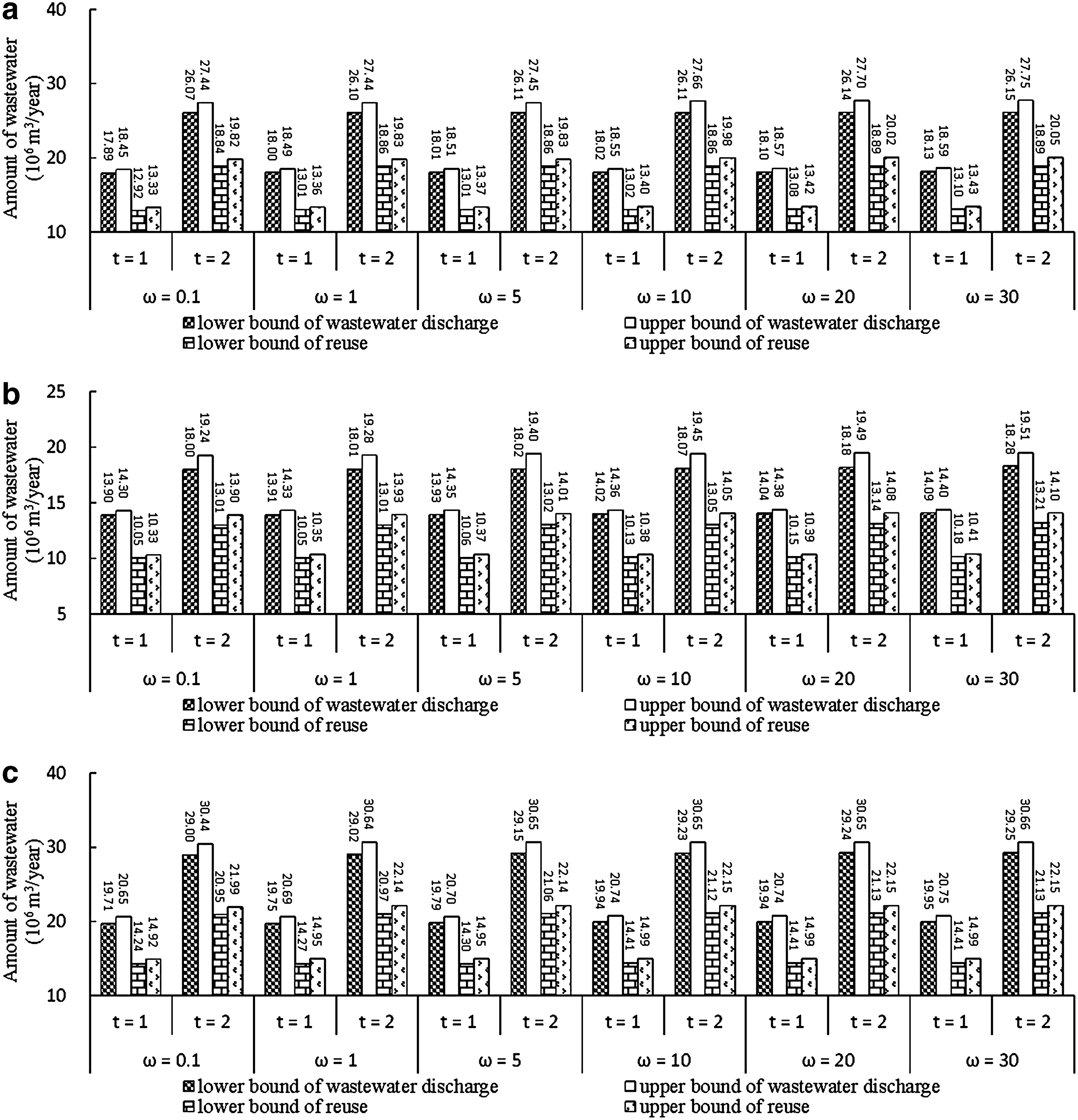
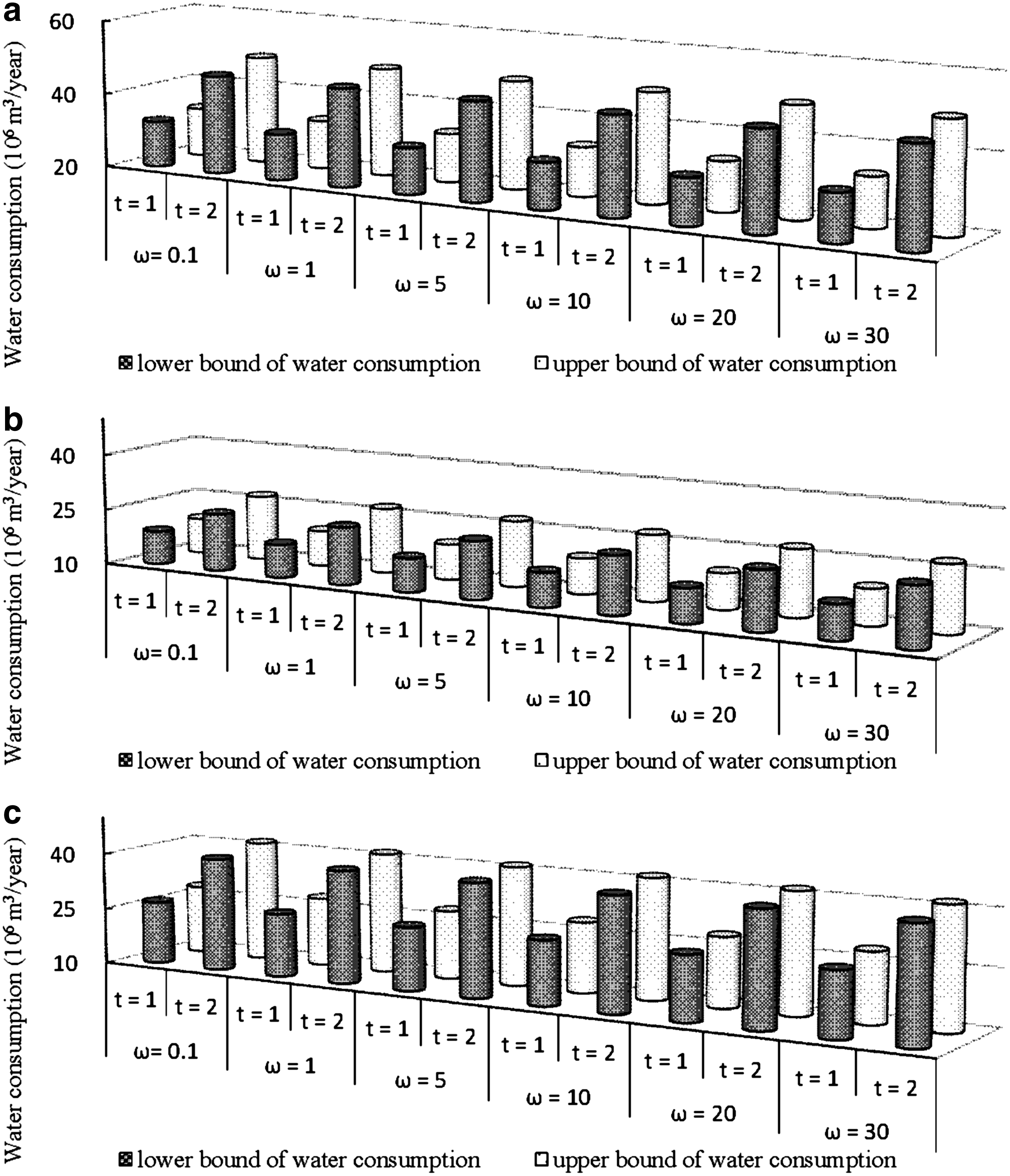
Different ω values correspond to changed production scales and thus result in varied wastewater discharge and reuse levels (Fig. 3). The results indicate that as ω value changes from 0.1 to 30, the amount of wastewater discharged from all chemical industries would increase. For example, in period 1, the total wastewater discharge would, respectively, be 51.50–53.40×10⁶ m³/year under ω=0.1 and 52.17–53.75×10⁶ m³/year under ω=30; the centralized treatment wastewater would, respectively, be 43.77–45.39×10⁶ m³/year (ω=0.1) and 44.34–45.69×10⁶ m³/year (ω=30). At the same time, there would be 37.21–38.58×10⁶ m³/year (ω=0.1) and 37.69–38.83×10⁶ m³/year (ω=30) treated water for reuse, respectively. According to the future environmental planning of New Binhai District, the capacities of sewage plants for chemical industries would be 46.7–48.5×10⁶ m³/year in period 1 and 66.2–69.8×10⁶ m³/year in period 2, which would be sufficient to meet the wastewater treatment over the planning horizon. The centralized treatment rate of sewage and the recycling rate of treated water would be 85% in period 1 and 90% in period 2. The results indicate that the amounts of wastewater discharged from fine-chemical industries are much larger than those discharged from petrochemical and marine chemical industries. This is possibly because the wastewater discharges for unit production of fine chemical industry are relatively larger than those from the other two industries. The water consumption for different industries under other ω values can be similarly interpreted based on the results presented in Fig. 4.

OPEN IN VIEWER

FIG. 3.

Solutions of wastewater discharged and water reused for the (a) petrochemical industry, (b) marine chemical industry, and (c) fine chemical industry.

OPEN IN VIEWER

FIG. 4.

Solutions for water consumption for (a) petrochemical industry, (b) marine chemical industry, and (c) fine chemical industry.

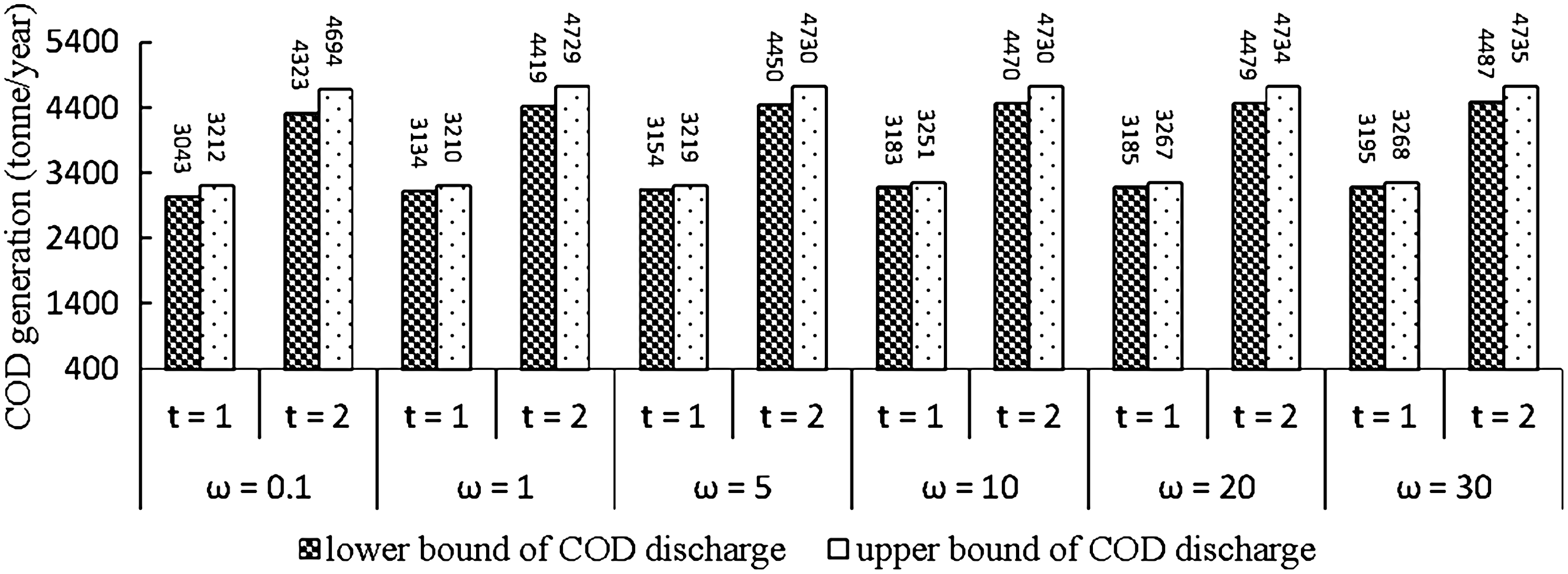
Figure 5 presents the results for COD discharged from chemical industries over the planning horizon under different ω values. The results demonstrate that the lower and upper bounds of COD discharge would increase with the increased ω values. For example, in period 1, the total COD discharge would be 3043–3212 ton/year under ω=0.1 and 3195–3269 ton/year under ω=30. As ω values change, the amounts of COD discharged from petrochemical, marine chemical, and fine chemical industries would be similarly interpreted based on the results shown in Fig. 6. Meanwhile, most of the COD mainly comes from raw sewage that is directly discharged into the river water body. For example, in period 1, the amounts of COD discharged from raw sewage would, respectively, be 456.5–481.8 ton/year under ω=0.1 and 479.2–490.2 ton/year under ω=30; the amounts of COD discharged from treated water would be 6.57–6.81 ton/year when ω=0.1 and 6.656.85 ton/year when ω=30. This is mainly because 15% in period 1 and 10% in period 2 of the wastewater generated by chemical industries are directly discharged into the river water body. A large amount of pollutants directly discharged from raw sewage into the river water body can cause potential risks for environment pollution and public health. The district should enhance the intensity of centralized sewage treatment and thus improve water quality management and maintain sustainable socioeconomic development.

OPEN IN VIEWER

FIG. 5.

Total chemical oxygen demand (COD) discharges of all industries.

OPEN IN VIEWER

FIG. 6.

COD discharges for the (a) petrochemical industry, (b) marine chemical industry, and (c) fine chemical industry.

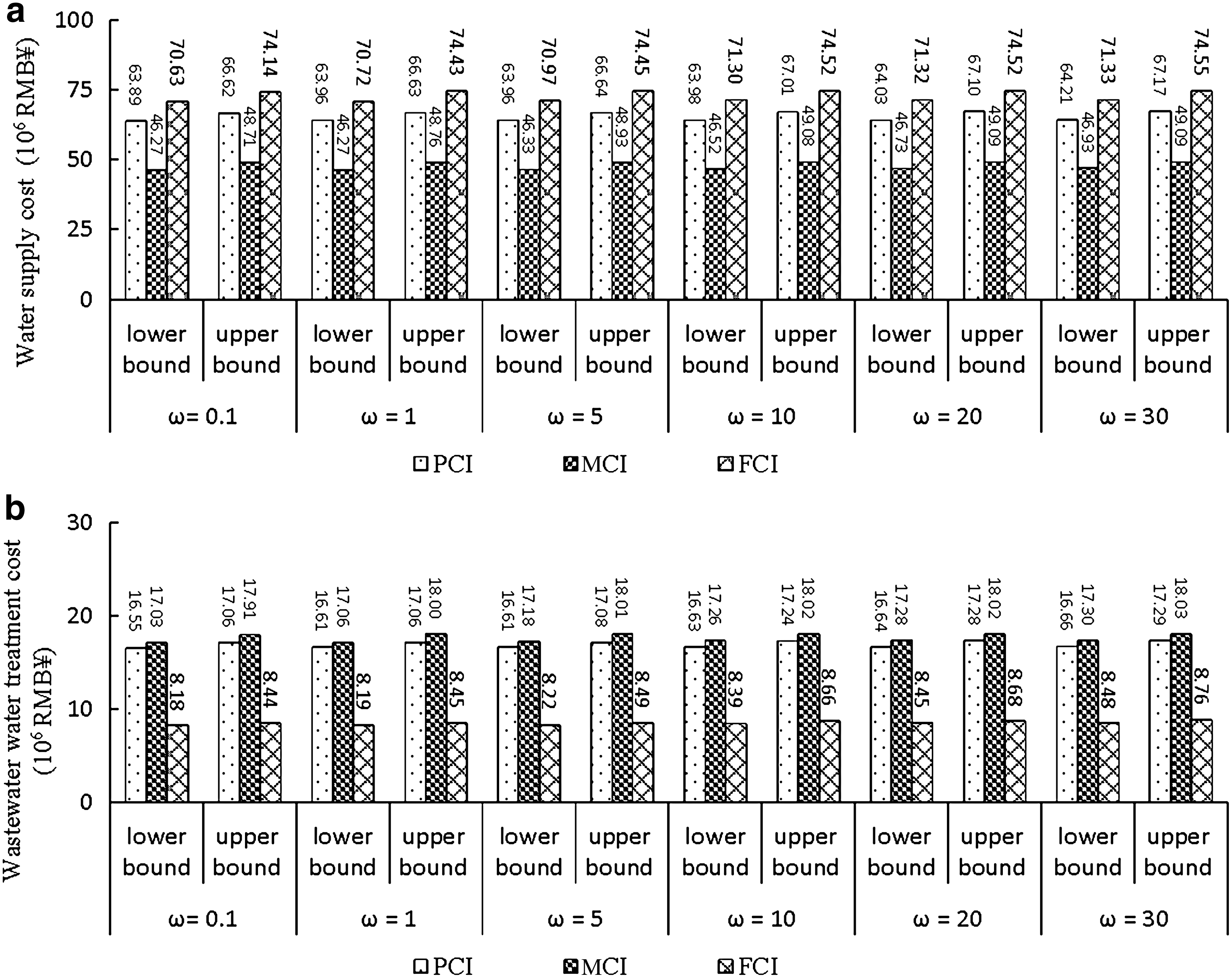
A further analysis for the water supply and wastewater treatment costs could be obtained from results as shown in Fig. 7. Generally, the lower and upper bounds of the water supply and wastewater treatment costs would both increase with the raised ω values. For example, in period 1, when the ω value changes from 0.01 to 30, the water consumption cost for petrochemical industry would raise from RMB¥ 32.33–32.96×10⁶ when ω=0.1 to RMB¥ 32.64–33.18×10⁶ when ω=30; the corresponding water demand cost for marine chemical industry would increase from RMB¥ 18.90–19.35×10⁶ (ω=0.1) to RMB¥ 19.17–19.47×10⁶ (ω=30); and the water requirement cost for fine chemical industry would range from RMB¥ 26.68–28.04×10⁶ under ω=0.1 to RMB¥ 27.21–28.45×10⁶ under ω=30. This is possibly because an increased ω value could lead to not only an increased looseness for environmental constraints (i.e., the COD discharge and the sewage treatment capacity), but also a decreased strictness for the environmental requirements. The results in Fig. 7 also demonstrate that the wastewater treatment costs of different chemical industries under various ω values have a similar trend as the charges for water supply. Moreover, the water consumptions of fine-chemical industries would be larger than those of the other two industries, which is due to the fact that the unit production for water requirement from the fine-chemical industries is relatively higher than that from other chemical industries. The governmental investments for different chemical industries under various ω values would be also significantly different, as shown in Fig. 8.

OPEN IN VIEWER

FIG. 7.

Costs for (a) water supply and (b) wastewater treatment.

OPEN IN VIEWER

FIG. 8.

Governmental investments for all industries.

Comparisons with the conventional optimization models

Substituting the modeling capacity constraints by deterministic average values, the study problem can then be converted into a conventional SRO model. Table 5 shows the solutions obtained from the SRO model. They are sets of deterministic values rather than discrete intervals, which represents one of many alternatives generated from the HIRO model. For example, in period 1, the total production scales from the SRO would be 8329.7×10³, 8358.4×10³, 8365.4×10³, 8367.3×10³, 8408.6×10³, and 9425.5×10³ ton/year under ω values of 0.1, 1, 5, 10, 20, and 30, respectively. Moreover, the solutions from SRO lie within the solution intervals of HIRO, demonstrating the stability and feasibility of the HIRO solutions. The stability and feasibility of the HIRO model attributed to the solutions of SRO model are special cases in the solutions obtained from the HIRO model. With the SRO, only one deterministic solution corresponding to each ω value is generated, which is due to the model's left-hand-side coefficients all being assumed to be deterministic. Then, further sensitivity analyses of the SRO model can only reflect the uncertain features of the modeling parameters individually and cannot comprehensively reflect the effects or interactions among multiple uncertain parameters. In comparison, HIRO can communicate uncertainties of all modeling parameters as well as their interactions into the optimization process.

The problem can also be solved through the ILP model, which has the same sewage discharge and COD emission constraints. Figure 9 shows a comparison of the production scales of various chemical industries from the SRO, ILP, and HIRO models, when ω=0.1. The results demonstrate that the production scales of the SRO model lie within the HIRO model, while the ILP model would obtain higher production scales compared with the HIRO model. Solutions of the ILP (in Fig. 9) also provide two extremes of the production scales of various chemical industries, which are both higher than those obtained through the HIRO model. This is because the variability of recourse costs and the risk of constraint violation were both ignored in stochastic interval linear programming (SILP), resulting in a decreased strictness for the constraints and an expanded decision space. The system benefit from the SILP model is RMB¥ 79.83–83.23×10⁹ (Table 6), higher than that from the HIRO model. This is mainly due to the fact that a decreased strictness for the river water quality requirement means an increased risk of violating environmental constraints, and thus a raised COD discharge and an increased system benefit. Generally, ILP only considered maximizing expected system benefit, and this may often fail to reduce the variability of the recourse values. Compared with HIRO, ILP has the following limitations: (1) it can only generate one interval solution without information about the risk of violating the capacity constraints; (2) it lacks the linkage to the economic consequences of violated polices as preformulated by authorities with recourse. In contrast, the developed HIRO can reflect economic penalties as corrective measures against any infeasibility arising due to a particular realization of uncertainty. Moreover, HIRO can effectively deal with the above complexities through enforcing the robustness of the uncertain environmental constraints (i.e., COD discharge), which is more suitable for risk-averse planners under high-variability conditions. Therefore, without the robust optimization, ILP is unable to support in-depth analysis of the tradeoff between system cost and system failure risk. Besides, the SILP model may potentially result in wasted capacity resources and thus increased system benefits.

OPEN IN VIEWER

FIG. 9.

Solutions from HIRO, SILP, and stochastic robust optimization (SRO) models (ω=0.1).

OPEN IN VIEWER

Table 6.

Solutions from the Interval Linear Programming Model

Period (t)	PCI	MCI	FCI
Production scale (×103 ton/year)
t=1	5347.3–5463.1	2231.7–2265.6	725.3–765.7
t=2	6146.4–6506.1	2618.5–2762.7	938.8–951.2
Discharged COD (ton/year)
t=1	1373.2–1383.9	1229.6–1238.5	535.2–562.2
t=2	1891.2–2021.1	1718.8–1820.0	792.2–829.8

System benefit (×10⁹ RMB¥)=79.83–83.23.

Conclusions

An interval SRO (HIRO) method has been developed for planning regional economic and environmental systems under uncertainty. The proposed HIRO method is based on incorporation of SRO and ILP within a general framework. The preferences of decision makers can be effectively reflected through specifying the certainty degree of imprecise objective functions. HIRO enhances the robustness of the optimization processes and resulting solutions by delimiting the decision space through dimensional enlargement of COD discharge constraints. Thus, the uncertainties can be directly communicated into the optimization process and the resulting solutions.

The developed HIRO method has been applied to a long-term planning of a regional case study for economic development in association with water pollution concerns in New Binhai District of Tianjin, China. The objective was to (1) formulate the local policies regarding industrial structure, economic development, and environmental protection; (2) analyze the interactions among criteria of industry layout, economic cost and benefit, pollution mitigation, and water quality security; (3) adjust the inter-relationship between the conflicting economic objectives and environmental requirements. The modeling constraints include allowable COD discharge, amount of water resources, capacity of sewage treatment plants, government investment, and technical constraints. The results demonstrate that the proposed HIRO model could communicate the interval-format uncertainties into the optimization process and generate inexact solutions that contain a spectrum of potential constraint violation risk options. Decision alternatives can be obtained by adjusting different combinations of the decision variables within their solution intervals. The results are helpful for supporting local decision makers in generating benefit-effective water quality management schemes.

This study is the first attempt for planning economic and environmental management systems through the development of incorporation techniques of the SRO and ILP methods. The results suggest that the proposed method would also be applicable to many other regional environmental management problems (i.e., solid waste and air quality) where complex uncertainties exist. In addition, it is also possible that many other uncertain methods (such as fuzzy programming and chance-constrained programming) have potential to be further integrated into HIRO for handling more complicated real-world practical problems.

Nomenclature