Markov Chain Monte Carlo Approach for Parameter Uncertainty Quantification and Its Impact on Groundwater Mass Transport Modeling: Influence of Prior Distribution

Abstract

Markov Chain Monte Carlo (MCMC) theory and stochastic simulation techniques were incorporated to analyze the effect of different prior knowledge on quantifying parameter uncertainty and its impact on mass transport in heterogeneous aquifer. The MCMC algorithm employing the Metropolis-Hastings rule (MH-MCMC) was used to obtain the posterior distribution of log-hydraulic conductivity. Random simulation technology, Sequential Gaussian Simulation, was used to generate a spatial stochastic hydraulic conductivity field. We investigated two different assumptive prior knowledge scenarios, a uniform prior distribution and a Gaussian prior distribution. Results showed that the prior knowledge could affect the posterior distributions of parameters. When the Gaussian prior distribution was adopted, there was a better convergence of parametric posterior distribution and a decrease in the zone of uncertainty influence and the area of confidence interval on groundwater mass transport modeling. However, it was difficult to draw the conclusion that the Gaussian prior distribution was preferred because the relative influence of parameter prior distribution depended on the location, number of measurements, and methods to reflect the heterogeneity of hydraulic conductivity. Therefore, the prior distribution is a sensitive input parameter and should be defined based upon best available data.

Introduction

Groundwater models are used to predict or estimate the behavior of groundwater systems (Zeng et al., 2009; Liang et al., 2010). Modeling propagates many kinds of uncertainties, which stem from observations—deficiency, parametric uncertainty, boundary uncertainty, and spatial variability (Freni et al., 2008; Willems, 2008; Rojas et al., 2010; Wu et al., 2010). Uncertainty analysis in groundwater modeling can help to attain a relatively accurate result and reduce the sources of error, whose relative importance may propagate to the model outputs (Willems, 2008). The uncertainty analysis likely spans values that are centered around the true value of a specific simulated variable: lower quantifiable uncertainty is connected with stricter uncertainty bands; larger bands are caused by highly uncertain models (Freni and Mannina, 2010).

Among the mentioned uncertainties, parametric uncertainty, caused by heterogeneity of hydraulic properties, has attracted widespread attention. Many former researchers have used spatial statistical methods to characterize the heterogeneity and uncertainty of hydraulic properties in groundwater modeling applications (Feyen and Caers, 2006). Hydraulic conductivity is considered to be the most important input parameter of groundwater flow models. Its variability in space is considerably higher than other hydraulic properties relevant to groundwater flow and it can vary by orders of magnitude over a few meters (Feyen et al., 2003). Random space function models are often adopted to characterize the spatial variability of hydraulic conductivity (Franssen et al., 2003; Kerrou et al., 2008; Liang et al., 2009). Three parameters, mean (μ), sill (c), and range (h) can be used to generate spatial distribution of hydraulic conductivity based upon measured hydraulic conductivity values. Scarcity of data and lack of detailed information concerning spatial variability make assumptions in uncertainty techniques impacting variability associated with groundwater flow and transport model predictions.

Uncertainty associated with parameter estimation within this context needs to be accounted for, along with impact on the output variability. Many articles have been published on parameter estimation in the random space function. A commonly used methodology for assessing the parametric uncertainty is the Bayesian approach such as the Markov Chain Monte Carlo (MCMC) method (Neuman et al., 2012). Parameter uncertainty through MCMC method is accounted for by introducing a prior probability distribution, which represents historical or expert information before any new data is collected, and a likelihood function, which characterizes the proximity of simulated and observed data. The MCMC approach expresses parameter uncertainties in terms of a probability distribution known as the posterior distribution. The parametric prior distribution is used to generate a posterior distribution to summarize uncertainty and quantify its effects on model prediction (Freni and Mannina, 2010).

The prior distribution is generally random designated due to the deficiency of prior information and the uniform distribution is usually preferred. The prior distribution as an important component of the Bayesian inference can affect the posterior distribution and the subsequent model results. This article combines the MCMC approach with random simulation technology and simultaneously compares the performance of two different prior distributions: a uniform distribution and a Gaussian distribution to quantify the effect of the selection of the prior distribution on the groundwater flow and mass transport models.

Methodology

Groundwater flow and mass transport governing equations

The equation describing groundwater flow and mass transport in a heterogeneous confined aquifer can be written as follows (Zheng and Wang, 1999): \documentclass{aastex}\usepackage{amsbsy}\usepackage{amsfonts}\usepackage{amssymb}\usepackage{bm}\usepackage{mathrsfs}\usepackage{pifont}\usepackage{stmaryrd}\usepackage{textcomp}\usepackage{portland, xspace}\usepackage{amsmath, amsxtra}\pagestyle{empty}\DeclareMathSizes{10}{9}{7}{6}\begin{document} \begin{align*} \frac { \partial } { \partial x_i } \left( K_i \frac { \partial h ( x_i ) } { \partial x_i } \right) + q_s = S_s \frac { \partial h ( x_i ) } { \partial t } \tag { 1 } \end{align*} \end{document}

where K is the hydraulic conductivity; h is the hydraulic head of the aquifer; q_s is the infiltration thickness per unit time; S_s is specific yield; t is time; x_i is the distance along the respective Cartesian coordinate axis; i is the respective Cartesian coordinate axis. \documentclass{aastex}\usepackage{amsbsy}\usepackage{amsfonts}\usepackage{amssymb}\usepackage{bm}\usepackage{mathrsfs}\usepackage{pifont}\usepackage{stmaryrd}\usepackage{textcomp}\usepackage{portland, xspace}\usepackage{amsmath, amsxtra}\pagestyle{empty}\DeclareMathSizes{10}{9}{7}{6}\begin{document} \begin{align*}Rn \frac { \partial C ( x_i ) } { \partial t } = \frac { \partial } { \partial x_i } \left( nD_ { ij } \frac { \partial C ( x_i ) } { \partial x_i } \right) - \frac { \partial } { \partial x_i } \left( nu_iC ( x_i ) \right) + q_sC_s \tag { 2 } \end{align*} \end{document}

where R is the retardation coefficient; C is the dissolved concentration; n is the porosity of the subsurface medium, dimensionless; t is time; x_i is the distance along the respective Cartesian coordinate axis; D_ij is the hydrodynamic dispersion coefficient tensor; u_i is the seepage or linear pore water velocity; q_s is the volumetric flow rate per unit volume of aquifer representing fluid; C_s is the concentration of the source or sink flux sources (positive) and sinks (negative).

Random space simulation method

Sudicky (1986) has found that hydraulic conductivity (K) is log-normally distributed in a heterogeneous aquifer. K(x) is used to stand for the stochastic hydraulic conductivity field and its log form is denoted as Y(x)=log K(x), where x indicates the spatial location. Gaussian stationary random simulation field (RSF) with constant μ and an isotropic exponential two-point covariance function are adopted to quantificationally describe the spatial continuity of Y(x) (Feyen et al., 2003): \documentclass{aastex}\usepackage{amsbsy}\usepackage{amsfonts}\usepackage{amssymb}\usepackage{bm}\usepackage{mathrsfs}\usepackage{pifont}\usepackage{stmaryrd}\usepackage{textcomp}\usepackage{portland, xspace}\usepackage{amsmath, amsxtra}\pagestyle{empty}\DeclareMathSizes{10}{9}{7}{6}\begin{document} \begin{align*}\overline{Y ( x ) } = \mu \tag{3}\end{align*} \end{document} \documentclass{aastex}\usepackage{amsbsy}\usepackage{amsfonts}\usepackage{amssymb}\usepackage{bm}\usepackage{mathrsfs}\usepackage{pifont}\usepackage{stmaryrd}\usepackage{textcomp}\usepackage{portland, xspace}\usepackage{amsmath, amsxtra}\pagestyle{empty}\DeclareMathSizes{10}{9}{7}{6}\begin{document} \begin{align*}V ( h ) = \left[ Y ( x + h ) - \overline{Y ( x + h ) } \right] \left[ Y ( h ) - \overline{Y ( h ) } \right] = \sigma^2 \rho ( h ) \tag{4}\end{align*} \end{document} \documentclass{aastex}\usepackage{amsbsy}\usepackage{amsfonts}\usepackage{amssymb}\usepackage{bm}\usepackage{mathrsfs}\usepackage{pifont}\usepackage{stmaryrd}\usepackage{textcomp}\usepackage{portland, xspace}\usepackage{amsmath, amsxtra}\pagestyle{empty}\DeclareMathSizes{10}{9}{7}{6}\begin{document} \begin{align*}V ( h ) = \sigma^2 \exp ( - h / \varphi ) \tag{5}\end{align*} \end{document}

where μ is the mean of the log-hydraulic conductivity, V(h) is the two-point covariance function of the process with lag separation vector h, the variance σ²(σ²=V(h=0)), and the correlation function ρ(h). The Equations (3 )–(5) indicate that Y(x) is decided by the three parameters: θ(μ, σ², ϕ).

MCMC approach to estimate parametric uncertainty

In this article, three parameters denoted by θ=(μ, σ², ϕ) are inferred by the MCMC approach from limited measurements to quantify the uncertainty stemming from the imperfect prior knowledge of parameters in the simulation process.

We assume that the log form of hydraulic conductivity is \documentclass{aastex}\usepackage{amsbsy}\usepackage{amsfonts}\usepackage{amssymb}\usepackage{bm}\usepackage{mathrsfs}\usepackage{pifont}\usepackage{stmaryrd}\usepackage{textcomp}\usepackage{portland, xspace}\usepackage{amsmath, amsxtra}\pagestyle{empty}\DeclareMathSizes{10}{9}{7}{6}\begin{document} $$y = ( y_1 , y_2 , \ldots , y_n ) ^T$$ \end{document} . According to Bayes' rules, we write the log hydraulic conductivity joint posterior (conditional) distribution of θ as \documentclass{aastex}\usepackage{amsbsy}\usepackage{amsfonts}\usepackage{amssymb}\usepackage{bm}\usepackage{mathrsfs}\usepackage{pifont}\usepackage{stmaryrd}\usepackage{textcomp}\usepackage{portland, xspace}\usepackage{amsmath, amsxtra}\pagestyle{empty}\DeclareMathSizes{10}{9}{7}{6}\begin{document} \begin{align*}p ( Y ( x ) \mid y ) = \int {p ( Y ( x ) \mid y , \theta ) p ( \theta \mid y ) d \theta} \tag{6}\end{align*} \end{document}

where p(Y(x)|y), the posterior distribution, is a function of the likelihood function p(Y(x)|y,θ) and the prior distribution p(θ|y).

A conventional MCMC algorithm employing the Metropolis-Hastings rule (MH-MCMC) was used in this study to solve Equation (6). The basic steps of MH-MCMC are described as follows:

(1) Initialize the first realization, i=0, \documentclass{aastex}\usepackage{amsbsy}\usepackage{amsfonts}\usepackage{amssymb}\usepackage{bm}\usepackage{mathrsfs}\usepackage{pifont}\usepackage{stmaryrd}\usepackage{textcomp}\usepackage{portland, xspace}\usepackage{amsmath, amsxtra}\pagestyle{empty}\DeclareMathSizes{10}{9}{7}{6}\begin{document} $$\theta_n^{i} = \theta_0$$ \end{document} ;

(2) Generate a new realization according to the Metropolis-Hastings rule:

• Draw a candidate realization \documentclass{aastex}\usepackage{amsbsy}\usepackage{amsfonts}\usepackage{amssymb}\usepackage{bm}\usepackage{mathrsfs}\usepackage{pifont}\usepackage{stmaryrd}\usepackage{textcomp}\usepackage{portland, xspace}\usepackage{amsmath, amsxtra}\pagestyle{empty}\DeclareMathSizes{10}{9}{7}{6}\begin{document} $$\theta_n^*$$ \end{document} based on the chosen appropriate transition probability \documentclass{aastex}\usepackage{amsbsy}\usepackage{amsfonts}\usepackage{amssymb}\usepackage{bm}\usepackage{mathrsfs}\usepackage{pifont}\usepackage{stmaryrd}\usepackage{textcomp}\usepackage{portland, xspace}\usepackage{amsmath, amsxtra}\pagestyle{empty}\DeclareMathSizes{10}{9}{7}{6}\begin{document} $$G ( \theta_n^* \mid \theta_n^i )$$ \end{document} ;

• Draw the prior probability density function g, the likelihood probability density function L, the transition probability density function based on \documentclass{aastex}\usepackage{amsbsy}\usepackage{amsfonts}\usepackage{amssymb}\usepackage{bm}\usepackage{mathrsfs}\usepackage{pifont}\usepackage{stmaryrd}\usepackage{textcomp}\usepackage{portland, xspace}\usepackage{amsmath, amsxtra}\pagestyle{empty}\DeclareMathSizes{10}{9}{7}{6}\begin{document} $$\theta_n^*$$\end{document} and \documentclass{aastex}\usepackage{amsbsy}\usepackage{amsfonts}\usepackage{amssymb}\usepackage{bm}\usepackage{mathrsfs}\usepackage{pifont}\usepackage{stmaryrd}\usepackage{textcomp}\usepackage{portland, xspace}\usepackage{amsmath, amsxtra}\pagestyle{empty}\DeclareMathSizes{10}{9}{7}{6}\begin{document} $$\theta_n^i$$ \end{document} ;

• Calculate the acceptance probability \documentclass{aastex}\usepackage{amsbsy}\usepackage{amsfonts}\usepackage{amssymb}\usepackage{bm}\usepackage{mathrsfs}\usepackage{pifont}\usepackage{stmaryrd}\usepackage{textcomp}\usepackage{portland, xspace}\usepackage{amsmath, amsxtra}\pagestyle{empty}\DeclareMathSizes{10}{9}{7}{6}\begin{document} $$A ( \theta_n^i , \theta_n^* )$$ \end{document} , where

\documentclass{aastex}\usepackage{amsbsy}\usepackage{amsfonts}\usepackage{amssymb}\usepackage{bm}\usepackage{mathrsfs}\usepackage{pifont}\usepackage{stmaryrd}\usepackage{textcomp}\usepackage{portland, xspace}\usepackage{amsmath, amsxtra}\pagestyle{empty}\DeclareMathSizes{10}{9}{7}{6}\begin{document} \begin{align*}A ( \theta_n^i , \theta_n^* ) = \min \left\{ 1 , \frac { G ( \theta_n^i \mid \theta_n^* ) f ( L_n \mid \theta_n^* , \theta_0 ) g ( \theta_n^* \mid \theta_0 ) } { G ( \theta_n^* \mid \theta_n^i ) f ( L_n \mid \theta_n^i , \theta_0 ) g ( \theta_n^i \mid \theta_0 ) } \right\} ;\end{align*} \end{document}

• Generate a random number of uniform distribution, u∼U[(0,1)];

• If \documentclass{aastex}\usepackage{amsbsy}\usepackage{amsfonts}\usepackage{amssymb}\usepackage{bm}\usepackage{mathrsfs}\usepackage{pifont}\usepackage{stmaryrd}\usepackage{textcomp}\usepackage{portland, xspace}\usepackage{amsmath, amsxtra}\pagestyle{empty}\DeclareMathSizes{10}{9}{7}{6}\begin{document} $$u < A ( \theta_n^i , \theta_n^* )$$ \end{document} then \documentclass{aastex}\usepackage{amsbsy}\usepackage{amsfonts}\usepackage{amssymb}\usepackage{bm}\usepackage{mathrsfs}\usepackage{pifont}\usepackage{stmaryrd}\usepackage{textcomp}\usepackage{portland, xspace}\usepackage{amsmath, amsxtra}\pagestyle{empty}\DeclareMathSizes{10}{9}{7}{6}\begin{document} $$\theta_n^{i + 1} = \theta_n^*$$ \end{document} , otherwise \documentclass{aastex}\usepackage{amsbsy}\usepackage{amsfonts}\usepackage{amssymb}\usepackage{bm}\usepackage{mathrsfs}\usepackage{pifont}\usepackage{stmaryrd}\usepackage{textcomp}\usepackage{portland, xspace}\usepackage{amsmath, amsxtra}\pagestyle{empty}\DeclareMathSizes{10}{9}{7}{6}\begin{document} $$\theta_n^{i + 1} = \theta_n^i$$ \end{document} ;

(3) i=i+1, return to (2).

After enough iterations, the MCMC chains are converged. Various statistical characteristics, such as the mean and the variance, can be obtained from the parametric posterior distribution.

Uncertainty assessment

Three metrics are defined to measure parameter uncertainty from the difference between the reference and the simulated concentration (Fu and Gómez-Hernández, 2009). \documentclass{aastex}\usepackage{amsbsy}\usepackage{amsfonts}\usepackage{amssymb}\usepackage{bm}\usepackage{mathrsfs}\usepackage{pifont}\usepackage{stmaryrd}\usepackage{textcomp}\usepackage{portland, xspace}\usepackage{amsmath, amsxtra}\pagestyle{empty}\DeclareMathSizes{10}{9}{7}{6}\begin{document} \begin{align*}I_1 = \frac { 1 } { node } \sum_ { m = 1 } ^ { node } \frac { 1 } { node } _r \sum_ { r = 1 } ^ { node_r } ( c_ { m , r } - \overline{c_m} ) ^2 \tag { 7 } \end{align*} \end{document} \documentclass{aastex}\usepackage{amsbsy}\usepackage{amsfonts}\usepackage{amssymb}\usepackage{bm}\usepackage{mathrsfs}\usepackage{pifont}\usepackage{stmaryrd}\usepackage{textcomp}\usepackage{portland, xspace}\usepackage{amsmath, amsxtra}\pagestyle{empty}\DeclareMathSizes{10}{9}{7}{6}\begin{document} \begin{align*}I_2 = \frac { 1 } { node } \sum_ { m = 1 } ^ { node } \frac { 1 } { node } _r \sum_ { r = 1 } ^ { node_r } ( c_ { m , r } - { c_ { m , ref } } ) \tag { 8 } \end{align*} \end{document} \documentclass{aastex}\usepackage{amsbsy}\usepackage{amsfonts}\usepackage{amssymb}\usepackage{bm}\usepackage{mathrsfs}\usepackage{pifont}\usepackage{stmaryrd}\usepackage{textcomp}\usepackage{portland, xspace}\usepackage{amsmath, amsxtra}\pagestyle{empty}\DeclareMathSizes{10}{9}{7}{6}\begin{document} \begin{align*}I_3 = \frac { 1 } { node } \sum_ { m = 1 } ^ { node } \frac { 1 } { node } _r \sum_ { r = 1 } ^ { node_r } ( c_ { m , r } - { c_ { m , ref } } ) ^2 \tag { 9 } \end{align*} \end{document}

where node is the number of cells, node_r is the number of realizations, c_m,r is the simulated value at cell m and realization r, \documentclass{aastex}\usepackage{amsbsy}\usepackage{amsfonts}\usepackage{amssymb}\usepackage{bm}\usepackage{mathrsfs}\usepackage{pifont}\usepackage{stmaryrd}\usepackage{textcomp}\usepackage{portland, xspace}\usepackage{amsmath, amsxtra}\pagestyle{empty}\DeclareMathSizes{10}{9}{7}{6}\begin{document} $$\overline{c_m}$$ \end{document} is the ensemble average over all realizations at location m, and c_m,ref is the reference concentration at cell m in the study area.

I₁ measures the precision of the realizations since it evaluates the ensemble variance over all the cells, I₂ measures the average and I₃ measures a combination of bias and precision. The smaller the I₁, I₂, and I₃ are, the smaller uncertainty of prediction.

Case study

In this article, a hypothetical steady two-dimensional flow and transport field in the groundwater constructed by Wilson and Miller (1978) were adopted to represent the reality and reflect the solute transport under the generated hydraulic conductivity field. The flow model was surrounded by constant-head boundaries on the west and east borders and no-flow boundaries on the north and south borders of the study area. The hydraulic head values at the constant-head boundaries were arbitrarily chosen so that the plume developed from the point source would not reach the boundary. There was regional flow from west to east across a 460×310 m with depth of a 10 m aquifer. The fluid moved at a Darcy velocity of 0.33 m/day, and the porosity of the porous medium was 0.3. The aquifer was assumed to have heterogeneous and isotropic properties. A point source released a small amount of fluid into the aquifer at 1 m³/day at location (x=160 m, y=160 m). The injected concentration of mass was 1,000 ppm. The aquifer was initially pristine with concentrations everywhere equal to zero. The only source of contaminant was the injection; thus, flow through the inlet had zero concentration. The period of interest was 1 year.

The main research steps were as follows:

First, the same conditioned log K(x) was used to update two kinds of assumptive prior information (a uniform distribution and a Gaussian distribution) to generate the parameter posterior distribution. Next, two hundred set θ were, respectively, chosen from their posterior distribution to yield conditional log K(x) field using sequential Gaussian simulation (sgsim) algorithm, one of the most commonly used forms of stochastic geostatistical simulation. Then, log K(x) field was transformed to K field and used as inputs of groundwater flow and transport model to generate the conditioned concentration field. Finally, the difference between the reference concentration field and the conditioned concentration field was quantified to evaluate the uncertainty of mass transport prediction with Equations (7 )–(9) for each iteration of the groundwater model.

Results and Discussion

Results of the reference fields

MODFLOW-96 was used to simulate the steady groundwater flow, and MT3DMS, through the third-order total variation diminishing solution scheme, was used to simulate the mass transport.

Figure 1a shows the reference field of logK(x) generated through the unconditional SGS algorithm. The parameters used to generate the reference hydraulic conductivity were μ=2, σ=0.5, and ϕ=100. The regularly chosen logK(x) to be conditioned from the reference field is shown in Fig. 1b. The reference field of the hydraulic head and the concentration are shown in Fig. 1c–f.

FIG. 1.

(a) Reference field of logK(x) generated through the unconditional SGS algorithm. (b) Conditional field of logK(x). (c) Reference field of hydraulic head. (d–f) Reference field of concentration for 100, 200, and 300 days.

Results of the MCMC approach

In this article, it was arbitrarily assumed that the uniform and Gaussian prior distributions could describe the hydraulic conductivity uncertainty and were thus used to update the parameter posterior distribution. The initial values of μ, σ², ϕ were, respectively, set as 2, 0.5, 100. In the two scenarios, we ran 20,000 MCMC simulations with q=5 parallel sequences to compute parameter posterior distribution. The Scale Reduction score ( \documentclass{aastex}\usepackage{amsbsy}\usepackage{amsfonts}\usepackage{amssymb}\usepackage{bm}\usepackage{mathrsfs}\usepackage{pifont}\usepackage{stmaryrd}\usepackage{textcomp}\usepackage{portland, xspace}\usepackage{amsmath, amsxtra}\pagestyle{empty}\DeclareMathSizes{10}{9}{7}{6}\begin{document} $$\sqrt{SR}$$ \end{document} ) defined by Gelman and Rubin (1992) was used to assess the convergence of the algorithm. If \documentclass{aastex}\usepackage{amsbsy}\usepackage{amsfonts}\usepackage{amssymb}\usepackage{bm}\usepackage{mathrsfs}\usepackage{pifont}\usepackage{stmaryrd}\usepackage{textcomp}\usepackage{portland, xspace}\usepackage{amsmath, amsxtra}\pagestyle{empty}\DeclareMathSizes{10}{9}{7}{6}\begin{document} $$\sqrt{SR}$$ \end{document} was less than 1.0 or close to 1, the parametric posterior distribution was considered to be converged. In Fig. 2, the calculated values of \documentclass{aastex}\usepackage{amsbsy}\usepackage{amsfonts}\usepackage{amssymb}\usepackage{bm}\usepackage{mathrsfs}\usepackage{pifont}\usepackage{stmaryrd}\usepackage{textcomp}\usepackage{portland, xspace}\usepackage{amsmath, amsxtra}\pagestyle{empty}\DeclareMathSizes{10}{9}{7}{6}\begin{document} $$\sqrt{SR}$$ \end{document} are plotted against the number of MCMC iterations. The line plots indicate that the MCMC chains were converged after ∼3,000 iterations when the Gaussian prior distribution was considered. When the uniform prior distribution was used, the MCMC chains for all parameters are converged after ∼5,000 iterations and for the parameter σ², the parallel sequences could not obtain a good convergent performance.

FIG. 2.

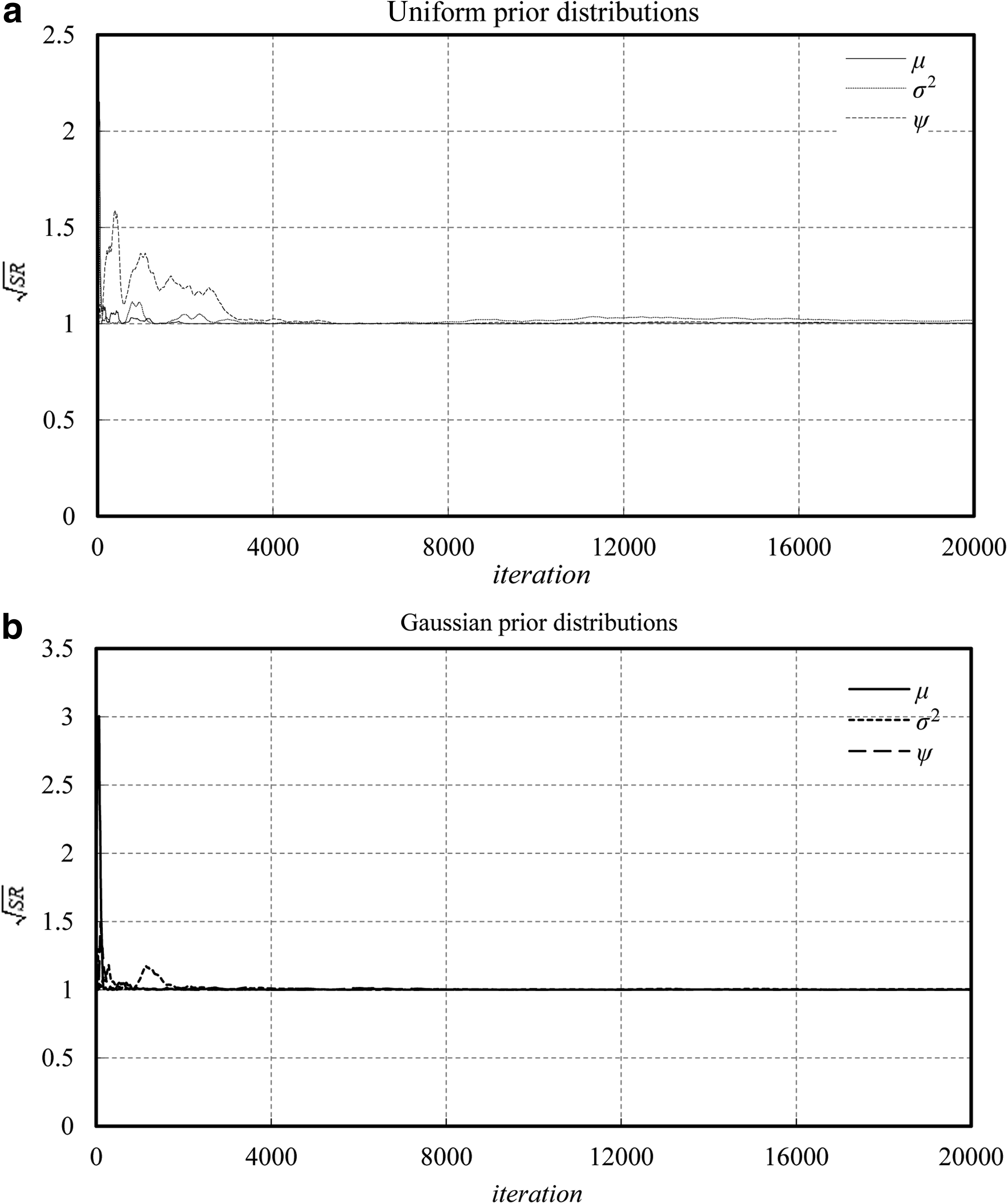
Scale Reduction ( \documentclass{aastex}\usepackage{amsbsy}\usepackage{amsfonts}\usepackage{amssymb}\usepackage{bm}\usepackage{mathrsfs}\usepackage{pifont}\usepackage{stmaryrd}\usepackage{textcomp}\usepackage{portland, xspace}\usepackage{amsmath, amsxtra}\pagestyle{empty}\DeclareMathSizes{10}{9}{7}{6}\begin{document} $$\sqrt{SR}$$\end{document} ) score of parameter θ under different parametric prior distributions.

Figure 3 shows the cumulative posterior probability functions (PDFs) of each parameter under different parametric prior distributions. When the uniform prior distribution was used, the posterior distributions of all parameters did not obey the uniform distribution. The posterior distributions of the parameter μ and the parameter φ were still the Gaussian distribution when the Gaussian prior distribution was used.

FIG. 3.

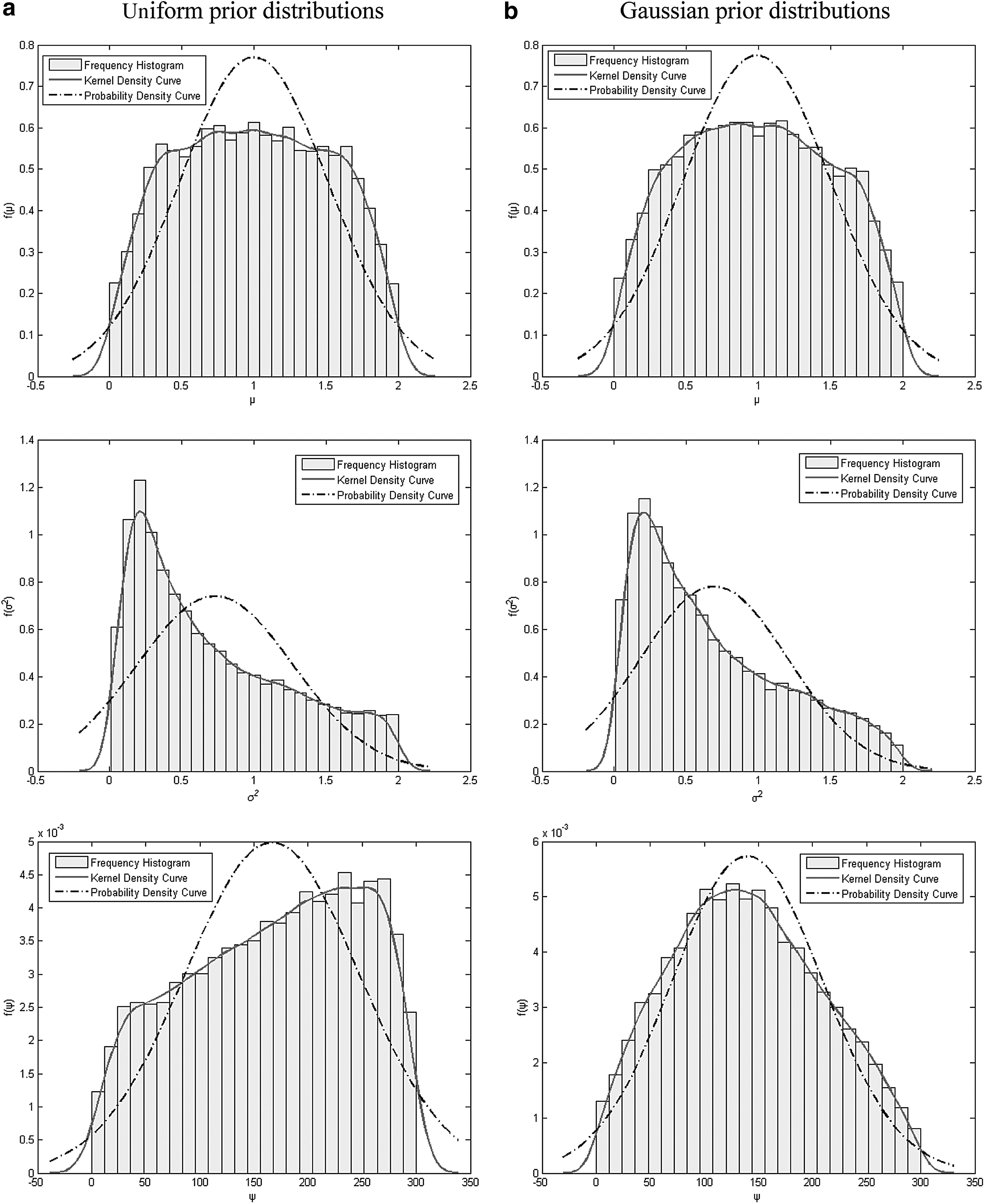
Cumulative posterior probability functions (PDFs) of each parameter under different parametric prior distributions.

Table 1 presents the summary statistics of the marginal parametric posterior distributions for different prior distributions. The range of the parameter was divided into 25 groups and the median of a group with the highest probability was taken as the optimal value of parameter. Percentiles, for example, 95% confidence interval was 2.5th percentile value, 97.5th percentile value, 90% confidence interval was 5th percentile value, 95th percentile value and the rest may be deduced by analogy, were used to determine the confidence interval of parameter and thus to reflect the parametric uncertainty.

Table 1.

Summary Statistics of Marginal Parametric Posterior Distributions for Different Prior Distributions

Parameter	Prior distribution	Samples	Optimal value	Mean value	Standard deviation	Kurtosis value	Skew value	Minimum value	Maximum value
M	Uniform	16,000	0.959	0.999	0.518	1.930	0.010	0.0001	2
σ²		16,000	0.137	0.730	0.540	2.326	0.682	0.0107	1.999
Φ		16,000	256.327	166.776	80.025	1.955	−0.251	0.021	299.987

			Percentile
Parameter	Prior distribution	Samples	5%	10%	25%	50%	75%	90%	95%
M	Uniform	16,000	0.183	0.294	0.571	0.996	1.432	1.707	1.822
σ²		16,000	0.092	0.140	0.268	0.581	1.122	1.589	1.793
Φ		16,000	29.366	48.704	102.307	174.894	234.807	269.481	281.532

Parameter	Prior distribution	Samples	Optimal value	Mean value	Standard deviation	Kurtosis value	Skew value	Minimum value	Maximum value
M	Gaussian	16,000	0.876	0.988	0.515	1.968	0.036	0	2
σ²		16,000	0.138	0.692	0.512	2.460	0.722	0.011	2.000
Φ		16,000	118.845	139.599	69.579	2.245	0.154	0.008	299.958

			Percentile
Parameter	Prior distribution	Samples	5%	10%	25%	50%	75%	90%	95%
M	Gaussian	16,000	0.174	0.288	0.566	0.980	1.407	1.705	1.819
σ²		16,000	0.083	0.131	0.263	0.556	1.045	1.501	1.701
Φ		16,000	29.410	47.104	86.540	136.367	190.536	237.449	260.075

The summary statistics showed that the standard deviation of θ was smaller and the optimal value was closer to the true value (μ=2, σ²=0.5, ϕ=100) when the Gaussian prior distribution was used.

Uncertainty quantification of the hydraulic head and mass transport

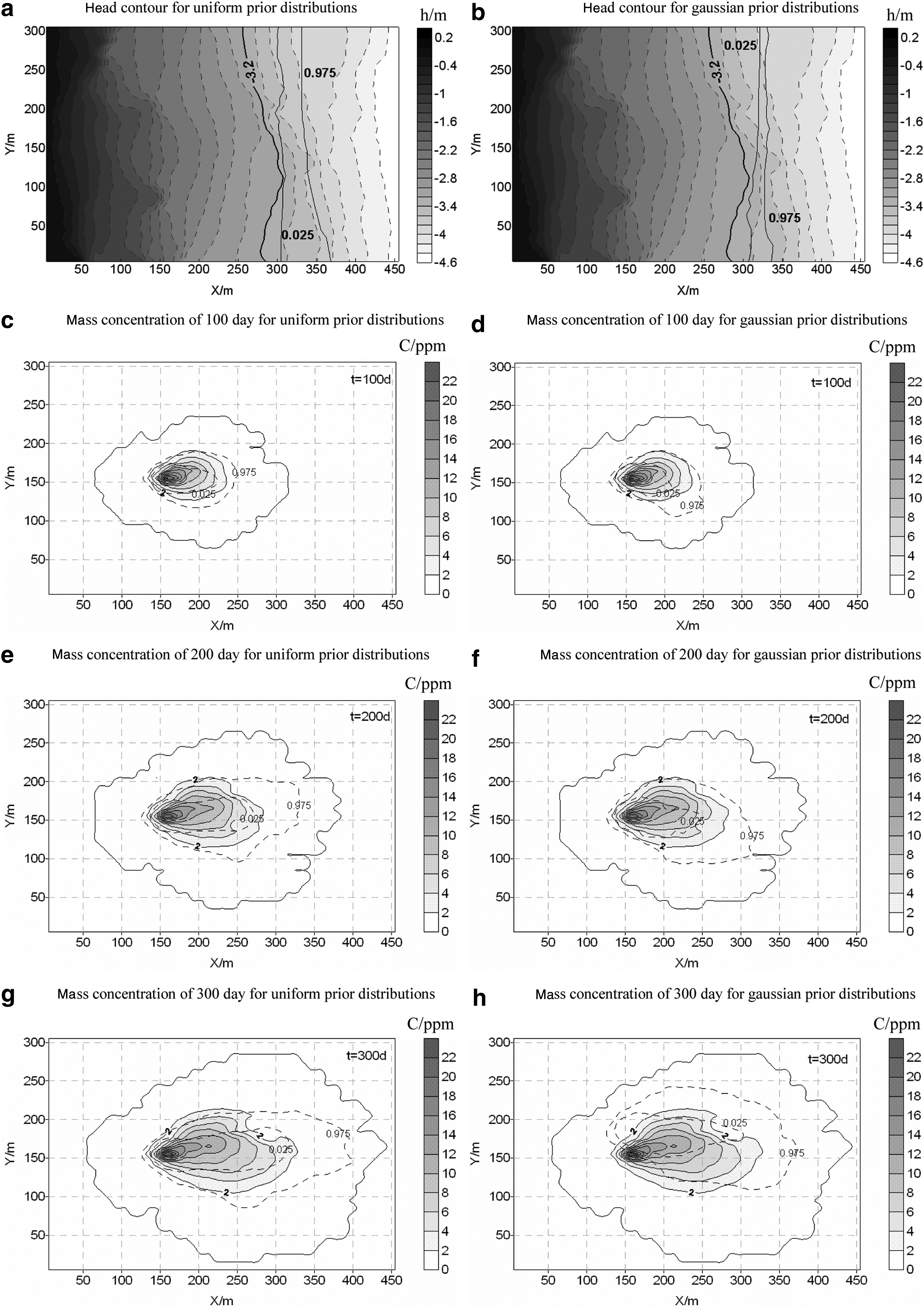
The variability in contaminant predictions due to parameter uncertainty of K was propagated by MCMC, and the MCMC was used to predict the concentration distributions of the contaminant. For uniform prior distributions, the simulated hydraulic head contour and the spatial variations of the mass concentration contour for t=100 day, t=200 day, t=300 day are illustrated in Fig. 4a, c, e, and g and for Gaussian prior distributions, the simulated hydraulic head contour and the spatial variations of the mass concentration contour for t=100 day, t=200 day, t=300 day are illustrated in Fig. 4b, d, f, and h. Figure 4a and b shows that the zone of 95% confidence interval of the hydraulic head field was smaller when the Gaussian prior distribution was considered. The zone of 95% confidence interval of the concentration field expanded with the increase of the simulation time along the flow direction with time increasing. Furthermore, the area impacted at the 95% confidence bound for the same simulation time was smaller when the Gaussian prior distribution was used. The values of the three metrics I₁, I₂, I₃ calculated on the hydraulic head and the mass concentration fields are listed in Table 2. By analyzing Table 2, we also noticed that the uncertainty of the hydraulic head and the mass concentration fields was smaller when the Gaussian distribution was adopted. The uncertainty of the mass concentration fields was increased as simulation time increased. The contours and the statistic uncertainty showed that the selection of the prior distribution could impact the hydraulic head and the mass concentration, but only because of different input parameter sampling for each model iteration. There was a smaller effect on the hydraulic head. This indicated that the uncertainty of the hydraulic conductivity was transferred to mass transport and it was magnified. However, it was difficult to draw the conclusion that the Gaussian prior distribution was more suitable because the results obtained depended on many factors, such as the location and the number of the chosen measurements from the reference field, which may affect the simulation result.

FIG. 4.

(a, c, e, g) Zone of 95% confidence interval of hydraulic head and concentration field when uniform prior distribution was considered. (b, d, f, h) Zone of 95% confidence interval of hydraulic head and concentration field when Gaussian prior distribution was considered.

Table 2.

Values of Three Metrics I₁, I₂, I₃ Calculated on Hydraulic Head and Mass Concentration Fields Under Different Prior Distributions

	The uniform prior distribution				The Gaussian prior distribution
		Uncertainty of mass transport				Uncertainty of mass transport
Uncertainty metrics	Uncertainty of head	100 days	200 days	300 days	Uncertainty of head	100 days	200 days	300 days
I ₁	0.0059	0.1679	0.3887	0.5807	0.0010	0.1320	0.2508	0.3315
I ₂	0.3850	0.0928	0.2175	0.3650	0.3799	0.0893	0.1987	0.3052
I ₃	0.2041	0.3317	0.7483	1.0908	0.1993	0.3117	0.6969	1.0653

Conclusions

In the article, the MCMC approach and stochastic simulation techniques were incorporated to analyze the effect of imperfect prior knowledge on parameter uncertainty (hydraulic conductivity only) and mass transport in a heterogeneous aquifer. Two prior knowledge scenarios, a uniform prior distribution and a Gaussian prior distribution, had been considered. The results showed that the prior knowledge dose affects the posterior distributions of parameters and the simulated hydraulic head and mass transport. Therefore, the prior distribution should be based on actual measurements rather than hypothesized. When the Gaussian prior distribution was adopted, there was a better convergence and a decrease in the zone of uncertainty influence on groundwater mass transport modeling. The above consideration may lead to the conclusion that the Gaussian prior distribution was preferred. However, it was difficult to draw conclusions about the relative influence of parameter prior distribution, as it depended on the location, number of the measurements, and the methods to reflect the heterogeneity of hydraulic conductivity.

Footnotes

Acknowledgments

The study was financially supported by the National Natural Science Foundation of China (51039001, 51009063), the National Foundation of the Three Gorges Project Committee under the State Council (SX2010-026), the Program for Changjiang Scholars and Innovative Research Team in University (IRT0719), and Fundamental research funds for the Central Universities.

Author Disclosure Statement

No competing financial interests exist.

References

Feyen

, and Caers

(2006). Quantifying geological uncertainty for flow and transport modeling in multi-modal heterogeneous formations. Adv. Water Res., 29, 912.

Feyen

, Ribeiro

J.P.J.

, Gómez-Hernández

J.J.

, Beven

K.J.

, and De Smedt

(2003). Bayesian methodology for stochastic capture zone delineation incorporating transmissivity measurements and hydraulic head observations. J. Hydrol., 271, 156.

Franssen

H.J.H.

, Gómez-Hernández

J.J.

, and Sahuquillo

(2003). Coupled inverse modelling of groundwater flow and mass transport and the worth of concentration data. J. Hydrol., 281, 281.

Freni

, and Mannina

(2010). Bayesian approach for uncertainty quantification in water quality modelling: the influence of prior distribution. J. Hydrol., 392, 31.

Freni

, Mannina

, and Viviani

(2008). Uncertainty in urban storm-water quality modelling: the effect of acceptability threshold in the GLUE methodology. Water Res., 42, 2061.

J.L.

, and Gómez-Hernández

J.J.

(2009). Uncertainty assessment and data worth in groundwater flow and mass transport modelling using a blocking Markov chain Monte Carlo method. J. Hydrol., 364, 328.

Gelman

, and Rubin

D.B.

(1992). Inference from iterative simulation using multiple sequences. Stat. Sci., 7, 457.

Kerrou

, Renard

, Hendricks

H.J.

, Franssen

, and Lunati

(2008). Issues in characterizing heterogeneity and connectivity in non-multi Gaussian media. Adv. Water Res., 31, 147.

Liang

, Zeng

G.M.

, Guo

S.L.

, Li

J.B.

, and Wei

A.L.

(2009). Uncertainty analysis of stochastic solute transport in heterogeneous aquifer. Environ. Eng. Sci., 26, 359.

10.

Liang

, Zeng

G.M.

, Guo

S.L.

, Wei

A.L.

, Li

X.D.

, Shi

, and Du

C.Y.

(2010). Optimal solute transport in heterogeneous aquifer: coupled inverse modeling. Int. J. Environ. Pollut., 42, 258.

11.

Neuman

S.P.

, Xue

, Ye

, and Lu

(2012). Bayesian analysis of data-worth considering model and parameter uncertainties. Adv. Water Res., 36, 75–85.

12.

Rojas

, Kahunde

, Peeters

, Batelaan

, Feyen

, and Dassargues

(2010). Application of a multi model approach to account for conceptual model and scenario uncertainties in groundwater modelling. J. Hydrol., 394, 416.

13.

Sudicky

E.A.

(1986). A natural gradient experiment on solute transport in a sand aquifer: spatial variability of hydraulic conductivity and its role in the dispersion process. Water Resour. Res., 22, 2069.

14.

Willems

(2008). Quantification and relative comparison of different types of uncertainties in sewer water quality modelling. Water Res., 42, 3539.

15.

Wilson

J.L.

, and Miller

P.J.

(1978). Two-dimensional plume in uniform ground water flow. J. Hydraul. Div. ASCE., 104, 503.

16.

, Clark

J.S.

, and Vose

J.M.

(2010). Assimilating multi-source uncertainties of a parsimonious conceptual hydrological model using hierarchical Bayesian modelling. J. Hydrol., 394, 436.

17.

Zeng

G.M.

, Liang

, Guo

S.L.

, Shi

, Xiang

, Li

X.D.

, and Du

C.Y.

(2009). Spatial analysis of human health risk associated with ingesting manganese in Huangxing Town, Middle China. Chemosphere, 77, 368.

18.

Zheng

, and Wang

P.P.

(1999). MT3DMS, a Modular Three-Dimensional Multi-Species Transport Model for Simulation of Advection, Dispersion and Chemical Reactions of Contaminants in Groundwater Systems. Documentation and User's Guide. Vicksburg, MS: US Army Engineer Research and Development Center Contract Report SERDP-99-1.