A Multistep Chaotic Model for Municipal Solid Waste Generation Prediction

Abstract

In this study, a univariate local chaotic model is proposed to make one-step and multistep forecasts for daily municipal solid waste (MSW) generation in Seattle, Washington. For MSW generation prediction with long history data, this forecasting model was created based on a nonlinear dynamic method called phase-space reconstruction. Compared with other nonlinear predictive models, such as artificial neural network (ANN) and partial least square–support vector machine (PLS-SVM), and a commonly used linear seasonal autoregressive integrated moving average (sARIMA) model, this method has demonstrated better prediction accuracy from 1-step ahead prediction to 14-step ahead prediction assessed by both mean absolute percentage error (MAPE) and root mean square error (RMSE). Max error, MAPE, and RMSE show that chaotic models were more reliable than the other three models. As chaotic models do not involve random walk, their performance does not vary while ANN and PLS-SVM make different forecasts in each trial. Moreover, this chaotic model was less time consuming than ANN and PLS-SVM models.

Introduction

Municipal waste management has always been a priority issue for environmental sustainability and resource management in urban area (Costi et al., 2004; Morrissey and Browne, 2004). Specifically, prediction of municipal solid waste (MSW) generation plays an important role in planning and management of urban solid waste system as prediction results can provide basic information for improving the effectiveness and efficiency of the planning system (Beigl et al., 2008; Chung, 2010; Lebersorger and Beigl, 2011; Abbasi et al., 2013). Nowadays, rapid urbanization has caused issues, such as population fluctuation, employment changes, and economic development (Dyson and Chang, 2005). These issues not only make MSW generation a more dynamic and complex waste stream compared with agricultural and industrial waste generation, but also bring increasing risks for human health and the environmental pollution (Hoornweg and Bhada-Tata, 2012). Moreover, the increasing daily MSW generation amount in developing countries has caused environmental and health problems in local level (Zurbrugg, 2002). As a result, time series prediction of MSW generation with high accuracy has become a challenge for proper MSW management planning challenges for the time series prediction of MSW generation with high accuracy (Troschinetz and Mihelcic, 2009). Moreover, as daily data are usually more complex and dynamic compared with weekly or monthly data, prediction of daily MSW generation amount in urban area has now become a problem for local governments who have the primary responsibility for MSW daily management, especially in developing countries, where MSW management is local governments' single largest budget (U.S. Environmental Protection Agency, 2002; Hoornweg and Bhada-Tata, 2012). As a consequence, in order to simulate the generation of MSW with higher accuracy to assist the local solid waste management planning, advanced forecasting methods, especially daily prediction, should be developed and applied for the time series prediction of the dynamic and complex MSW generation.

Ever since the 1970s, various MSW prediction models that utilize different mechanisms have been developed to forecast the long time trend of MSW generation to assist the waste management (Beigl et al., 2008; Troschinetz and Mihelcic, 2009; Xu et al., 2013). According to Beigl et al. (2008), commonly used models can be categorized based on the number of independent variables. Correlation, bivariate regression analysis, group comparison, and time series analysis only need to consider one independent variable to build the models, while methods, such as multiple regression analysis, system dynamics, and input-output analyses, consider the complicated interactions between multiple variables, making these models far more complex and difficult to validate. Some of the latest intelligent models, such as artificial neural network (ANN) (Noori et al., 2010), partial least square support vector machine (PLS-SVM) (Abbasi et al., 2012, 2013), grey system theory, and fuzzy dynamic models (Chen and Chang, 2000), have been proved to have good prediction performances for weekly or monthly time series data. In addition, various prediction models, including seasonal autoregressive integrated moving average (sARIMA) model and fuzzy logic model, have been developed to forecast daily MSW generation (Navarro-Esbrı et al., 2002; Karadimas, et al., 2006).

To deal with highly nonlinear daily MSW generation data, this article proposes a novel univariate local chaotic model to forecast MSW multistep generations based on a nonlinear dynamic method, phase-space reconstruction, to forecast MSW multistep generations in Seattle, Washington. Then, nonlinear regression models, including ANN and PLS-SVM, and linear sARIMA model, which is commonly used for weekly data prediction, are also implemented for the same daily MSW data to compare and evaluate the performance of the proposed chaotic model. The accuracy, stability, and time consuming of the newly built model are assessed in comparison with those of ANN, PLS-SVM, and sARIMA models.

In this article, we propose the univariate local chaotic model through introducing the basic theory of phase-space reconstruction and adopting a practical way for acquiring appropriate time delay and embedding dimension. Local multistep prediction method is explained in this section as well. We compare the time series modeling results among the proposed local chaotic model, ANN model, PLS-SVM model, and sARIMA model; discusses the accuracy, stability, and time consuming of the proposed method; and summarizes its pros and cons. Finally, we provide the main conclusions of the study.

Data and Methodology

In this study, daily MSW garbage generation data were obtained from the Seattle Public Utilities website from January 2011 to September 2013 for 1,001 days in total. The first 901 values of daily MSW generation were utilized to build all four forecast models and the last 100 values were used as comparison to evaluate the performance of each model.

To conduct the local chaotic modeling, nearest neighbor phase-space reconstruction method was implemented to forecast multistep daily MSW generation. Then, ANN, PLS-SVM, and sARIMA methods were implemented for the same data to compare and assess the chaotic model. The last 100 daily generation data were used to evaluate the forecasting performance of all the four different forecasting models. Finally, accuracies of forecasting values from all tested models were assessed to evaluate the performances of the models.

Phase-space reconstruction with appropriate time delay and embedding dimension

Phase-space reconstruction is a technique to rebuild the unknown dynamic system from univariate time series data. In this method, dynamic system, or nonlinear system, can be expressed in phase space using continuous m-first-order ordinary differential equations, such as \documentclass{aastex}\usepackage{amsbsy}\usepackage{amsfonts}\usepackage{amssymb}\usepackage{bm}\usepackage{mathrsfs}\usepackage{pifont}\usepackage{stmaryrd}\usepackage{textcomp}\usepackage{portland, xspace}\usepackage{amsmath, amsxtra}\pagestyle{empty}\DeclareMathSizes {10} {9} {7} {6} \begin{document} $$ \frac { d { \rm x } } { d { \rm t } } = f ( x ( t ) )$$ \end{document} , or discreet time series with the form x_n₊₁=f(x_n). If the evolution of the system is known, the future status of the system can be predicted in phase space. Takens (1981) proposed the Takens embedding theorem as a method to rebuild the dynamic behavior from a discrete time series data with time delay and embedding dimension. In Takens (1981) and Packard (Packard et al., 1980) theory, for a time series \documentclass{aastex}\usepackage{amsbsy}\usepackage{amsfonts}\usepackage{amssymb}\usepackage{bm}\usepackage{mathrsfs}\usepackage{pifont}\usepackage{stmaryrd}\usepackage{textcomp}\usepackage{portland, xspace}\usepackage{amsmath, amsxtra}\pagestyle{empty}\DeclareMathSizes {10} {9} {7} {6} \begin{document} $${ \rm x} = \{ x_1 , x_2 , x_3 \ldots x_n \} $$ \end{document} with length n, the phase space coordinate can be expressed in the form of vectors. \documentclass{aastex}\usepackage{amsbsy}\usepackage{amsfonts}\usepackage{amssymb}\usepackage{bm}\usepackage{mathrsfs}\usepackage{pifont}\usepackage{stmaryrd}\usepackage{textcomp}\usepackage{portland,xspace}\usepackage{amsmath,amsxtra}\pagestyle{empty}\DeclareMathSizes{10}{9}{7}{6} \begin{document} \begin{align*}{ \rm X} = \{ X_1 , X_2 , X_3 \ldots X_N \} \tag{1}\end{align*} \end{document}

Where length N=n-(m - 1)τ, m denotes the embedding dimension, and τ denotes the time delay.

Then the coordinate of each point in phase space can be written as: \documentclass{aastex}\usepackage{amsbsy}\usepackage{amsfonts}\usepackage{amssymb}\usepackage{bm}\usepackage{mathrsfs}\usepackage{pifont}\usepackage{stmaryrd}\usepackage{textcomp}\usepackage{portland,xspace}\usepackage{amsmath,amsxtra}\pagestyle{empty}\DeclareMathSizes{10}{9}{7}{6} \begin{document} \begin{align*}X_i = \{ x_i , x_{i + \tau} , x_{i + 2 \tau} \ldots x_{i + ( m - 1 ) \tau} \} \tag{2}\end{align*} \end{document}

Nonlinear evolutionary behavior of the dynamic system can be reconstructed in phase space only if appropriate time delay and embedding dimension are estimated. Large numbers of studies have discussed the method of selecting appropriate time delay and embedding dimension (Sivakumar et al., 2001; Cai et al., 2004; Karunasinghe and Liong, 2006). Considering the purpose of the best predicting ability and the pseudo-period of the data, we adopted a heuristic criterion proposed by Navarro-Esbrı et al. (2002) to minimize the mean square error (MSE) of prediction results. MSE can be expressed using the following equation: \documentclass{aastex}\usepackage{amsbsy}\usepackage{amsfonts}\usepackage{amssymb}\usepackage{bm}\usepackage{mathrsfs}\usepackage{pifont}\usepackage{stmaryrd}\usepackage{textcomp}\usepackage{portland,xspace}\usepackage{amsmath,amsxtra}\pagestyle{empty}\DeclareMathSizes{10}{9}{7}{6} \begin{document} \begin{align*} { \rm MS } { \rm E } ( \tau , { \rm m } ) = \sqrt { \frac { \sum_ { { \rm t } = 1 } ^ { \rm n } ( { \rm R } _ { \rm t } - { \rm F } _ { \rm t } ) ^2 } { { \rm n } } } \tag { 3 } \end{align*} \end{document}

Where R_t is the observation and F_t is the forecast.

Different τ and m were tested to obtain the minimum MSE value. Results show that τ=4 and m=7 are the best parameters, which is supported in Navarro-Esbrı's study that pseudo-period length is the best one (m=7 stands for a week).

Local method for multistep forecast

Local forecast approach is developed based on the self-similarity of chaotic attractor in which the trajectory of the current point is similar to the trajectories of its neighboring points. Farmer and Sidorowich (1987) have mathematically proved that local chaotic model has better performance than global model. Figure 1a is the Lorenz attractor (Lorenz, 1963) and Fig. 1b is the zoom-in version of a small part of Lorenz attractor. In phase space, the underlying dynamics of the system can be represented by a multidimensional space and the evolution of the trajectory can be studied. As shown in Fig. 1b, X_n is the end point of the scalar time series in phase space. The future point of this trajectory can be acquired using the following three steps:

FIG. 1.

(a) Trajectories of Lorenz attractor with self-similarity. (b) Zoom-in version of Lorenz attractor describing the basic method in local multistep ahead prediction.

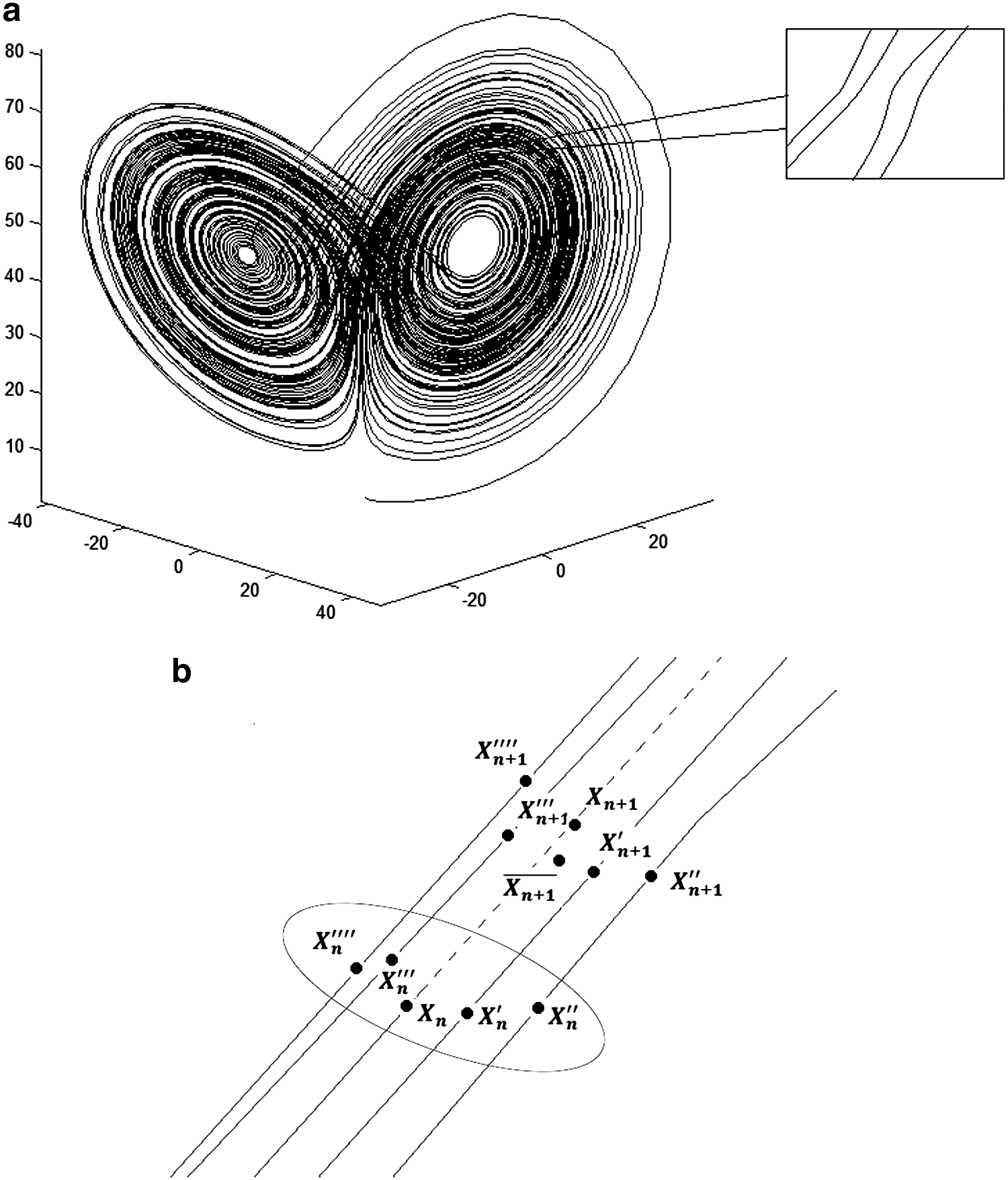
(1) Find p neighboring points ( \documentclass{aastex}\usepackage{amsbsy}\usepackage{amsfonts}\usepackage{amssymb}\usepackage{bm}\usepackage{mathrsfs}\usepackage{pifont}\usepackage{stmaryrd}\usepackage{textcomp}\usepackage{portland, xspace}\usepackage{amsmath, amsxtra}\pagestyle{empty}\DeclareMathSizes {10} {9} {7} {6} \begin{document} $$X_n^{ \prime} , X_n^{ \prime \prime} , X_n^{ \prime \prime \prime} , X_n^{ \prime \prime \prime \prime}$$ \end{document} ) by applying the Euclidian distances.

(2) Assign weights to each neighboring points: \documentclass{aastex}\usepackage{amsbsy}\usepackage{amsfonts}\usepackage{amssymb}\usepackage{bm}\usepackage{mathrsfs}\usepackage{pifont}\usepackage{stmaryrd}\usepackage{textcomp}\usepackage{portland, xspace}\usepackage{amsmath, amsxtra}\pagestyle{empty}\DeclareMathSizes {10} {9} {7} {6} \begin{document} $$W_n^k = e^ { - \frac { d^k } { d_ { min } } } $$ \end{document} , where d_min is the minimum distance of all the neighboring points and d^k is the distance of kth neighboring point.

(3) Then the one-step ahead forecast point is \documentclass{aastex}\usepackage{amsbsy}\usepackage{amsfonts}\usepackage{amssymb}\usepackage{bm}\usepackage{mathrsfs}\usepackage{pifont}\usepackage{stmaryrd}\usepackage{textcomp}\usepackage{portland, xspace}\usepackage{amsmath, amsxtra}\pagestyle{empty}\DeclareMathSizes {10} {9} {7} {6} \begin{document} $$ {\overline { X_ { n + 1 } } = \frac { w_n^k * X_ { n + 1 } ^k } { \sum_ { k = 1 } ^p w_n^k }} .$$ \end{document}

Traditional methods directly use the n-step ahead points of the neighboring points for prediction. However, Siek and Solomatine (2010) have reported the multistep iterative method (or rolling forecast) based on repeating one-step predictions. It iterates one-step ahead prediction by using each predicted value as the observed value for next step ahead prediction until n-step ahead is made. Compared with traditional methods, the multistep iterative method has higher accuracy because false nearest neighbors with larger deviation can be avoided. As a result, this study adopts the multistep iterative method in MSW multistep prediction.

Self-similarity of chaotic attractor enables the similar evolution of the dynamics of neighboring trajectories. Thus, the n-step ahead prediction can be made from the points of the n-step ahead of neighboring points in phase space. False nearest neighbors can be avoided in some degree if the weights are assigned to each trajectory.

Results and Discussions

In this study, the chaotic model was implemented to predict the daily MSW generation data. Then, ANN, PLS-SVM, and sARIMA models were also implemented to compare and assess the performance of the new chaotic model. By the time of writing this article, only Navarro-Esbrı et al. (2002) have discussed using time series analysis method to predict daily MSW generation. They tested the performance of sARIMA and a nonlinear method, and all three parameters (mean square prediction error, steps predicted inside a tolerance limit, and mean relative prediction error) showed that sARIMA outperforms the nonlinear method. Based on this fact, we also include sARIMA as a contrast method in this article. As for nonlinear models, ANN (Zade and Noori, 2008; Noori et al., 2010) and SVM (Noori et al., 2009; Abbasi et al., 2012, 2013) are the most commonly used model for weekly MSW data. This article only chose two typical nonlinear ANN and SVM models (nonlinear autoregressive with exogenous input [NARX] and PLS-SVM) as contrast models because we focused on discussing the performance of the basic model structure and the preprocessing method (wavelet transform and principal component transform) proposed in these articles can be implemented on chaotic model in further discussion. Other models like grey system are only suitable for short history time series analysis, which is outside the scope of this article.

For the chaotic model, the heuristic analysis result recommended the embedding dimension, time delay, and nearest neighbor values to be 7, 4, and 9. An advanced ANN model, NARX, was employed for comparison since NARX outperforms the standard neural-network-based predictors (Menezes and Barreto, 2008; Xie et al., 2009). Time-delay values of both NARX and PLS-SVM were set to 7 taking seasonal patterns into consideration. When building the sARIMA model, the autocorrelation function plot, partial autocorrelation function plot, Box-Cox test, Akaike Information Criterion, and Schwarz Criterion were all considered to build the best-fitted model. In this way, the final sARIMA model used in this article can be sARIMA (2, 0, 1) (1, 0, 0)₇. A time lag for 7 days was used as the seasonal parameter for the Auto Regressive section considering the 7-day cycle of the daily MSW data. Then, time lags for 1 and 2 days were used as the parameters for Auto Regressive section and time lag for 1 day was used as the parameter for Moving Average section of the sARIMA model.

Three measures of accuracy were applied for comparison of these models, including mean absolute percentage error (MAPE), root MSE (RMSE), and correlation coefficient (R²).

MAPE is a commonly used method to measure the accuracy as a percentage in time series forecasting. It is defined as following: \documentclass{aastex}\usepackage{amsbsy}\usepackage{amsfonts}\usepackage{amssymb}\usepackage{bm}\usepackage{mathrsfs}\usepackage{pifont}\usepackage{stmaryrd}\usepackage{textcomp}\usepackage{portland,xspace}\usepackage{amsmath,amsxtra}\pagestyle{empty}\DeclareMathSizes{10}{9}{7}{6} \begin{document} \begin{align*} { \rm MAPE } = \frac { 1 } {\rm n } \sum_ { { \rm t } = 1 } ^ { \rm n } \frac { { \rm R } _ { \rm t } - { \rm F } _ { \rm t }} {{ \rm R } _ { \rm t } } \tag { 4 } \end{align*} \end{document}

Where R_t is the observation and F_t is the forecast.

RMSE is a frequently used measure of the difference between forecast value and real one. It is defined as following: \documentclass{aastex}\usepackage{amsbsy}\usepackage{amsfonts}\usepackage{amssymb}\usepackage{bm}\usepackage{mathrsfs}\usepackage{pifont}\usepackage{stmaryrd}\usepackage{textcomp}\usepackage{portland,xspace}\usepackage{amsmath,amsxtra}\pagestyle{empty}\DeclareMathSizes{10}{9}{7}{6} \begin{document} \begin{align*} { \rm RMSE } = \sqrt { \frac { \sum_ { { \rm t } = 1 } ^ { \rm n } ( { \rm R } _ { \rm t } - { \rm F } _ { \rm t } ) ^2 } { { \rm n } } } \tag { 5 } \end{align*} \end{document}

Correlation coefficient (R²) is a measurement of linear correlation of two variables. It can also be used to measure the correlations between observation and forecast. \documentclass{aastex}\usepackage{amsbsy}\usepackage{amsfonts}\usepackage{amssymb}\usepackage{bm}\usepackage{mathrsfs}\usepackage{pifont}\usepackage{stmaryrd}\usepackage{textcomp}\usepackage{portland,xspace}\usepackage{amsmath,amsxtra}\pagestyle{empty}\DeclareMathSizes{10}{9}{7}{6} \begin{document} \begin{align*} R^2 = 1 - \frac { \sum_ { { \rm t } = 1 } ^ { \rm n } ( { \rm F } _ { \rm t } - { \rm R } _ { \rm t } ) ^2 } { \sum_ { { \rm t } = 1 } ^ { \rm n } ( { \rm R } _ { \rm t } - {{ {\overline {\rm R } }} )} ^2 } \tag { 6 } \end{align*} \end{document}

Where \documentclass{aastex}\usepackage{amsbsy}\usepackage{amsfonts}\usepackage{amssymb}\usepackage{bm}\usepackage{mathrsfs}\usepackage{pifont}\usepackage{stmaryrd}\usepackage{textcomp}\usepackage{portland, xspace}\usepackage{amsmath, amsxtra}\pagestyle{empty}\DeclareMathSizes {10} {9} {7} {6} \begin{document} $$\overline{R}$$ \end{document} is the mean values of R_t.

The scalar time series data has 1,001 daily values in total and is split into two parts when conducting prediction. The first 901 − n+1 values were used for training models and the last 100 values were for n-step ahead predicting. As NARX and PLS-SVM have random walk that leads to nonstable results, for each step ahead prediction, the NARX and PLS-SVM models are implemented for 5 times and a medium performance is recorded for comparison.

Showing the MAPE values of all three models in 14 days, Fig. 2 suggests that the chaotic model outperforms the other two models for around 2%. Of all the 14 days, the average MAPE of chaotic model is 11.75% while NARX, PLS-SVM, and sARIMA are 13.81%, 14.01%, and 17.01%. Besides, there may be a watershed for every 6–8 days ahead prediction for the three nonlinear models. The performances of these models degrade in the second week during the 3 weeks. In respect to sARIMA, its performance apparently declines (around 5%) after 7 days (a week) and has worse accuracy than the linear models (Table 1), which indicates that linear models are not suitable to fit the complexity of long history MSW data. Figure 3a, c, e, and f shows the one-step ahead forecasts of these four models with observed values and forecast values. MSW generation fluctuates quasiperiodically, which is quite different from the work done by Navarro-Esbrı et al. (2002). If the threshold is 7, then the accuracy of chaotic model, NARX, PLS-SVM, and sARIMA degrades for about 1.09%, 1.77%, 2.14%, and 4.69%.

FIG. 2.

Comparison of n-Step ahead forecast performances of chaotic model, NARX, partial least square support vector machine (PLS-SVM), and seasonal autoregressive integrated moving average (sARIMA): (a) average mean absolute percentage error (MAPE); (b) max MAPE; (c) root mean square error (RMSE); (d) R². Last 100 data are used as the validation value for comparing the accuracy of the three models. x-Axis is the n days ahead. y-Axis is the average MAPE of the 100 validation values.

FIG. 3.

One-step ahead prediction of municipal solid waste (MSW) generation by chaotic model of the last 100 days. (a), (c), (e), and (g) are the original time series and predicted time series by chaotic model, NARX, PLS-SVM, and sARIMA. (b), (d), (e), and (h) are corresponding R².

Table 1.

General Comparison of Three Models

	Chaotic model	NARX	PLS-SVM	sARIMA
Predictability (MAPE, 14 days average)	11.75%	13.81%	14.01%	17.01%
Predictability (RMSE, 14 days average)	88.56	98.38	89.77	99.49
Predictability (Max error, 14 days average)	51.36%	98.17%	75.07%	89.36%
Forecast efficiency degrading	1.09%	1.77%	2.14%	4.69%
Repeatable	Yes	No	No	Yes
Time consuming	1.847 s	126.865 s	10.371 s	—

Forecast efficiency degrading means the degradation between the first and the second week.

MAPE, mean absolute percentage error; NARX, nonlinear autoregressive with exogenous input; PLS-SVM, partial least square support vector machine; RMSE, root mean square error; sARIMA, seasonal autoregressive integrated moving average.

The results also show that chaotic model is more stable than NARX and PLS-SVM models. Currently, there is no reliable general method available to determine confidence interval of chaotic model, two black box models, and sARIMA model at the same time. Therefore we use statistical results from experiment to define stability instead of mathematical derivation from model itself. In addition, we believe if the forecasting model is to be implemented in other places, then it should be better tested on history data for validating the performance instead of just assessing several statistic parameters. In this article, we measure stability by comparing the forecast sets in each trial: average MAPE, max MAPE, and RMSE partly shown in Table 1. As described previously, the chaotic model should not require any random computation process while the other two models require either in initial condition determination or in parameter estimation. This means that the chaotic model only exports one result in repeated trials while NARX and PLS-SVM produce different models in each trial. The performance of the two models varies in different trials, which makes these models unrepeatable. Table 2 lists the different MAPE value sets of the two models in 10 trials. Forecasting results vary greatly in NARX model from 11.59% to 14.45% possibly due to the instability of 10-neuron network. The same is much better in PLS-SVM models of 13.18% to 13.24%. Table 1 lists general comparison of the four models: the average error, max error (MAPE), RMSE and R²; all indicate that chaotic model produces more accurate result in both short and long term overall. Figure 2d shows the max errors of the three models. Generally, the chaotic model outperforms the other two models from 1 to 14 days ahead prediction. The max error is another indication of the instability of ANN and PLS-SVM models. The confidence level of chaotic model is also better than that of the other two models. Figure 3b shows the RMSE of the three models. As RMSE is an indicator of the scatter around the observation, it represents the deviation of the forecasts and the observations. When comparing the three models in this graph, it also proves the stability of the three models as described previously.

Table 2.

MSW Forecasting Result Comparison of One-Step Ahead in 10 Trials Between NARX and PLS-SVM

	10 trials
NARX	12.81%	12.95%	13.12%	12.63%	14.45%	11.59%	14.64%	14.31%	12.92%	13.25%
PLS-SVM	13.18%	13.24%	13.19%	13.21%	13.22%	13.18%	13.18%	13.19%	13.19%	13.21%

MSW, municipal solid waste; NARX, nonlinear autoregressive with exogenous input; PLS-SVM, partial least square support vector machine.

Once the parameters are determined, the time consumed of the three models in the 100-day iterating process can be recorded. Algorithm of chaotic model is much simpler and easier to implement since it has only one-step, history value search. The other two black box models have iterating training and implementing steps that make the algorithms quite complicated. Comparisons are listed in Table 2. Though sARIMA has high efficiency in calculation this model, it is not compared with other models since choosing the best parameters for the model is difficult. Some automatic parameter estimation algorithms have been developed (Hyndman and Khandakar, 2008), but there is still no systematic and integrated method to estimate the best parameters automatically for sARIMA. However, it should be noted that due to the algorithm efficiency and operating environment, the assessment of elapsed time is only for relative comparison. Besides, considering the circumstance of one observation a day, all the four models' efficiencies are acceptable.

Moreover, it should be noticed that there is a deficiency of the chaotic model. To find the true neighbor points in phase space, a long historic data is required. As this model is a local model, shorter historic data may lead to false neighbors increasing that will lead to wrong trajectories. Figure 4 shows the same performance of 10-step ahead prediction but in different historic data. The predictability of the chaotic model keeps increasing as the number of history data increases. Evolution of the dynamic system will be preserved if more history data are imported into the system. Thus, less and less false nearest neighbors will be included in the final calculation. This phenomenon means that this method is only restricted to daily MSW prediction for only MSW in this length is qualified for satisfying performance of chaotic model.

FIG. 4.

Effects of number of history data on predictability of chaotic model in MSW prediction. Ten days ahead prediction as an example. x-Axis is the number of history data. y-Axis is the average MAPE of the 100 validation values.

Conclusions

This article introduced a chaotic model, local phase-space reconstruction, to forecast daily MSW generation data. Two commonly used nonlinear MSW forecast models, NARX and PLS-SVM, and a linear model sARIMA were implemented to compare the multistep ahead predictability performance of the chaotic model. The experiment results show that the chaotic model outperforms the other three models in three aspects. (1) The chaotic model is more accurate than the other three models. Fourteen-day average MAPE of chaotic model is 11.75% while the other three models are 13.87%, 14.01%, and 17.01%. RMSE of the four models is 88.56, 98.38, 89.77, and 99.49, respectively. (2) The chaotic model is more stable than the other three models. The chaotic model is deterministic and its result is repeatable. The other two black box models have random processes and the result of each trial varies. Ten-trial experiment shows that the results of NARX model are very instable while variation of PLS-SVM is acceptable. (3) Chaotic model consumes far less time than the other three models. The algorithm of chaotic model is simpler and easy to implement than the other three models. Time-consuming experiment shows that chaotic model runs much faster than the other two black box models. For sARIMA, its parameter estimation is very complex and laborious. However, as time-consuming experiment is implemented on one operating environment, this may lead to inaccurate assessment. Considering the one observation a day circumstances, all the three models are acceptable.

One disadvantage of chaotic model is that the accuracy of chaotic model heavily depends on the length of historical data. The longer the data is, the better the performance is. This means that this chaotic model is not suitable for the prediction of traditionally yearly and monthly data. Weekly data can be conditionally tested. Besides, as chaotic model possesses multistep ahead predictability, future work may focus on the sum-up value of 1 week ahead forecast results or 1 month ahead forecast results to test whether it can be applied to these MSW forecast problems.

Other preprocessing methods like principal component analysis, gamma test, and wavelet transform, which have been integrated into ANN and SVM, can be tested to see whether chaotic model could further been improved. In addition, this study simply conducted univariate MSW multistep ahead forecast. As multivariate phase-space reconstruction has been proposed that makes this supposition possible (Boccaletti et al., 2002), future work can be focused on multivariate MSW forecast by taking more indicators, such as atmospheric data and socioeconomic data, into consideration. Dynamic data-driven application system can also be considered for hybrid forecasting, data assimilation, and measurement controlling as more and more models are proposed and social data are extracted in big data era (Song et al., 2014).

Footnotes

Acknowledgments

This article was supported by program of International S&T Cooperation “Fined Earth Observation and Recognition of the Impact of Global Change on World Heritage Sites” (Grant No. S2013GR0477) and the National Natural Science Foundation of China (Grant No. 41271427). The authors would like to thank Seattle Public Utilities for providing daily MSW garbage generation data from January 2011 to September 2013. The authors would also like to thank three anonymous reviewers for their helpful suggestions.

Author Disclosure Statement

No competing financial interests exist.

References

Abbasi

, Abduli

M.A.

, Omidvar

, and Baghvand

(2012). Forecasting municipal solid waste generation by hybrid support vector machine and partial least square model. Int. J. Environ. Res., 7, 27.

Abbasi

, Abduli

M.A.

, Omidvar

, and Baghvand

(2013). Results uncertainty of support vector machine and hybrid of wavelet transform‐support vector machine models for solid waste generation forecasting. Environ. Prog. Sustain. Energy, 33, 220.

Beigl

, Lebersorger

, and Salhofer

(2008). Modelling municipal solid waste generation: a review. Waste Manage., 28, 200.

Boccaletti

, Valladares

D.L.

, Pecora

L.M.

, Geffert

H.P.

, and Carroll

(2002). Reconstructing embedding spaces of coupled dynamical systems from multivariate data. Physical Review E., 65, 035204.

Cai

, Cai

, Shi

, Zhou

, and Zhang

(2004). Chaotic time series prediction based on local-region multi-steps forecasting model. In Advances in Neural Networks-ISNN 2004. Springer: Berlin Heidelberg, pp. 418–423.

Chen

H.W.

, and Chang

N.B.

(2000). Prediction analysis of solid waste generation based on grey fuzzy dynamic modeling. Resour. Conserv. Recycling, 29, 1.

Chung

S.S.

(2010). Projecting municipal solid waste: the case of Hong Kong SAR. Resour. Conserv. Recycling, 54, 759.

Costi

, Minciardi

, Robba

, Rovatti

, and Sacile

(2004). An environmentally sustainable decision model for urban solid waste management. Waste Manage. 24, 277.

Dyson

, and Chang

N.B.

(2005). Forecasting municipal solid waste generation in a fast-growing urban region with system dynamics modeling. Waste Manage. 25, 669.

10.

Farmer

J.D.

, and Sidorowich

J.J.

(1987). Predicting chaotic time series. Phys. Rev. Lett., 59, 845.

11.

Hoornweg

, and Bhada-Tata

(2012). What a Waste: A Global Review of Solid Waste Management. Urban Development Series. The Worldbank Knowledge Papers, No. 15. Available at https://openknowledge.worldbank.org/handle/10986/17388

12.

Hyndman

, and Khandakar

(2008). Automatic time series forecasting: the forecast package for R. J. Stat. Softw., 27, 1.

13.

Kalnay

(2003). Atmospheric Modeling, Data Assimilation, and Predictability. Cambridge University Press, New York.

14.

Karadimas

N.V.

, Orsoni

, and Loumos

(2006). Municipal solid waste generation modelling based on fuzzy logic. In Proceedings of the 20th European Conference on Modelling and Simulation. Bonn: Sankt Augustin, Germany, May 28–31, pp. 309–314.

15.

Karunasinghe

D.S.

, and Liong

S.Y.

(2006). Chaotic time series prediction with a global model: artificial neural network. J. Hydrol., 323, 92.

16.

Lebersorger

, and Beigl

(2011). Municipal solid waste generation in municipalities: quantifying impacts of household structure, commercial waste and domestic fuel. Waste Manage. 31, 1907.

17.

Lorenz

E.N.

(1963). Deterministic nonperiodic flow. J. Atmos. Sci., 20, 130.

18.

Menezes

J.M.P.

Jr. , and Barreto

G.A.

(2008). Long-term time series prediction with the NARX network: an empirical evaluation. Neurocomputing, 71, 3335.

19.

Morrissey

A.J.

, and Browne

(2004). Waste management models and their application to sustainable waste management. Waste Manage. 24, 297.

20.

Navarro-Esbrı

, Diamadopoulos

, and Ginestar

(2002). Time series analysis and forecasting techniques for municipal solid waste management. Resour. Conserv. Recycling, 35, 201.

21.

Noori

, Abdoli

M.A.

, Ghasrodashti

A.A.

, and Jalili Ghazizade

(2009). Prediction of municipal solid waste generation with combination of support vector machine and principal component analysis: a case study of Mashhad. Environ. Prog. Sustain. Energy, 28, 249.

22.

Noori

, Karbassi

, and Salman Sabahi

(2010). Evaluation of PCA and gamma test techniques on ANN operation for weekly solid waste prediction. J. Environ. Manage. 91, 767.

23.

Packard

N.H.

, Crutchfield

J.P.

, Farmer

J.D.

, and Shaw

R.S.

(1980). Geometry from a time series. Physical Review Letters, 45, 712.

24.

Siek

, and Solomatine

D.P.

(2010). Nonlinear chaotic model for predicting storm surges. Nonlin. Processes Geophys. 17, 405.

25.

Sivakumar

, Berndtsson

, and Persson

(2001). Monthly runoff prediction using phase space reconstruction. Hydrol. Sci. J., 46, 377.

26.

Song

, Xiang

, Wang

, Wu

, and Chang

Application of dynamic data driven application system in environmental science. Environ. Rev. [Epub ahead of print]; DOI: 10.1139/er-2013–0071.

27.

Takens

(1981). Detecting strange attractors in turbulence. In Dynamical Systems and Turbulence, Warwick 1980. Springer: Berlin Heidelberg, pp. 366–381.

28.

Troschinetz

A.M.

, and Mihelcic

J.R.

(2009). Sustainable recycling of municipal solid waste in developing countries. Waste Manage. 29, 915.

29.

U.S. Environmental Protection Agency (2002). Solid Waste Management: A Local Challenge With Global Impacts. Available at http://www.epa.gov/solidwaste/nonhaz/municipal/pubs/ghg/f02026.pdf

30.

Xie

, Tang

, and Liao

Y.H.

(2009, July). Time series prediction based on NARX neural networks: an advanced approach. In Machine Learning and Cybernetics, 2009 International Conference (Vol. 3, pp. 1275–1279). IEEE: Baoding, China.

31.

, Gao

, Cui

, and Liu

(2013). A hybrid procedure for MSW generation forecasting at multiple time scales in Xiamen City, China. Waste Manage., 33, 1324.

32.

Zade

, and Noori

(2008). Prediction of municipal solid waste generation by use of artificial neural network: a case study of Mashhad. Int. J Environ. Res., 2, 13.

33.

Zurbrugg

(2002). Urban solid waste management in low-income countries of Asia how to cope with the garbage crisis. Presented for Scientific Committee on Problems of the Environment (SCOPE) Urban Solid Waste Management Review Session, Durban, South Africa, 1.