Resilience of Secondary Wastewater Treatment Plants: Prior Performance Is Predictive of Future Process Failure and Recovery Time

Abstract

Performance of secondary wastewater treatment facilities over a long time period is an important consideration in plant operation and discharge regulation. Two characteristics of sustainable wastewater system performance, resilience and stability, were modeled using a Generalized Linear Model (GLM) and on average 41 months of data from plants in the U.S. Environmental Protection Agency's Integrated Compliance Information System database. Sample sizes were 209 plants for biological oxygen demand (BOD); 211 for total suspended solids (TSS); and 110 for ammonia. Independent variables were the previous month's effluent concentration relative to the permit limit; plant capacity, which ranged from 4 to 1,361,000 m³/day; and capacity utilization, which ranged from 5% to 180% of rated plant capacity. First, a GLM was fit to model relative effluent concentration as a function of the independent variables mentioned earlier and a first-order Markov component. The fitted model had an R² of 0.25, 0.28, and 0.25 for individual measurements of BOD, TSS, and ammonia, respectively, and an R² of 0.91, 0.90, and 0.83 for facility averages. These models were used to generate ensembles of 10-year long sequences, from which statistics of system performance, resilience, and stability were computed. The same was performed for BOD, TSS, and ammonia. The study revealed that when discharge of these constituents exceeded their permit limits, the likelihood of subsequent violations increased significantly, indicating lack of resilience. Recovery time, measured as the duration of monthly violations, ranged from 2 to 5 months, depending on capacity and capacity utilization, with small and overloaded plants more likely to have the longest sequential violations for BOD and ammonia.

Introduction

Wastewater treatment, from its introduction in the early 19th century through the 1972 Federal Water Pollution Control Act amendments to the Clean Water Act and beyond, has resulted in reduced risks to human health and aquatic environments from untreated human waste. However, impaired surface water continues to be an issue in the United States. The National Water Quality Inventory (U.S. Environmental Protection Agency, 2009) reports that the water quality of 44% of assessed United States rivers and streams and of 64% of assessed lakes and reservoirs was inadequate to support their designated uses. Municipal discharges and sewage contain toxic organics, pathogens, and nutrients and can cause organic enrichment, which leads to oxygen depletion. These discharges account for ∼15% of the impairment (sixth ranked source of impairment) for rivers and streams, 6% (seventh ranked source of impairment) for lakes and reservoirs, and are the second ranked source of impairment for the Great Lakes behind historical pollution. Currently, the Environmental Protection Agency (EPA) and state regulatory agencies are considering more stringent standards for nutrients due to recognition of the impacts of high nitrogen loads from both point and nonpoint sources on water bodies as large as the Gulf of Mexico and the Chesapeake Bay (U.S. Environmental Protection Agency, 2008c).

The EPA has recognized a need for significant repair or even replacement of aging centralized collection and treatment facilities. Specifically, the EPA estimated capital needs for wastewater systems in the United States between 2000 and 2019 to be $331–$450 billion with an associated gap between current capital spending and needs ranging from $73 to $122 billion over that period (U.S. Environmental Protection Agency, 2002). Repair and replacement of existing sanitary sewers, new interceptors, and combined sewer overflow represent nearly 50% of anticipated needs of clean water systems (U.S. Environmental Protection Agency, 2008a). Factors such as the cost of building out collection systems and pumping wastewater, improvements in small system technology, and automated operation have led organizations such as National Decentralized Wastewater Resources Capacity Development Project and the Center for Alternative Wastewater Treatment and the EPA-sponsored National Environmental Services Center to advocate for decentralized systems and small satellite plants as a solution to this need (National Environmental Services Center, 2008; Center for Alternative Wastewater Treatment, 2009; National Decentralized Water Resources Capacity Development Project, 2009). Decentralized wastewater systems may allow smaller collection systems relative to the number of connections, leading to significant savings in collection system construction, operation and maintenance, pumping, and financing costs (U.S. Environmental Protection Agency, 1997; Pinkham et al., 2004). However, Fane et al. (2004) described concerns arising from decentralized wastewater systems, including plant siting in residential areas, general lack of effluent data, and complex risks of failure.

A major concern with decentralized wastewater systems is treatment performance. Implicit in the operation of many traditional isolated small wastewater systems is reliance on high dilution of treated effluent in receiving waters. Accordingly, small systems may operate with smaller staff, less redundancy, and fewer monitoring requirements. However, replacing a centralized system with a network of small collection and treatment facilities effectively eliminates the dilution factor, making treatment performance and reliability an increased concern. Previous studies of the reliability of wastewater treatment did not include facility size as a variable and instead focused primarily on individual facilities (Niku and Schroeder, 1979), process type (Oliveira and Von Sperling, 2008), or effluent characterization (Hao et al., 2013). Other studies included facility size as a variable, but had too limited a range of facility sizes to identify a relationship between decentralization and reliability (Niku and Schroeder, 1981; Oakley et al., 2010). This is a missed opportunity for improvement in the quality of effluent-influenced receiving waters.

In addition to its role in enforcement, monitoring and reporting required under the National Pollutant Discharge Elimination System (NPDES) system provides an opportunity to assess treatment plant performance as a function of both design and operation factors and predicts impacts on water quality in effluent-influenced receiving waters. Weirich et al. (2011) investigated the relationship between plant size and performance. A statistical model to predict effluent water quality was developed using data from 210 treatment plants ranging in size from 1 to 335,000 m³/day from the EPA's Integrated Compliance Information System (ICIS). They found that the size (capacity) and hydraulic loading rate influenced a treatment plant's ability to meet discharge permit levels of biological oxygen demand (BOD), suspended solids, and ammonia, regardless of treatment process type. Furthermore, the risk of permit violations for these contaminants was larger for smaller plants, especially those operating at a higher percent of their rated capacity. The average frequency of permit violations for ammonia, for example, ranged from <1% for larger plants to nearly 20% for small plants (Weirich et al., 2011).

A further concern in considering decentralized wastewater systems is the resilience of wastewater systems, that is, their ability to recover from process upsets. Infrastructure resilience has been considered primarily in the context of disaster response—the capability of a system exposed to natural or man-made hazards to resist failure, recover within an acceptable time period, or adapt to changed conditions and continue to function. Resilience is a function of physical properties of infrastructure system components, interactions between components, and even societal factors. One aspect of resilience is the cumulative difference from expected normal performance, representing costs or losses during recovery after a failure (Corotis, 2011). The ability to learn from previous events or failures is also a factor in infrastructure resilience, related to adaptation (McDaniels et al., 2008). Resilience of wastewater infrastructure may have a number of factors, including the ability to maintain treatment performance and discharge water quality during extreme events or hazards, the ability to adapt to changing discharge standards, and the ability to recover from process upsets or failures.

To date, there have been no efforts to define, much less quantify, resilience in wastewater treatment systems. However, wastewater treatment plant discharges will continue to be a significant potential source of contamination of natural waters, and achieving more sustainable wastewater systems will depend to some degree on increasing the resilience of treatment plants with a related reduction in vulnerability of receiving water quality. In addition, lack of resilience increases the costs of wastewater treatment through fines and penalties levied due to lack of permit compliance. In this study, it is assumed that factors that affect treatment system resilience may not be related to traditional design and operations practices, which tend to be based on normed values for inputs and performance requirements, but rather are based on overall system characteristics such as facility size. A statistical definition of treatment plant resilience is proposed along with a methodology for quantifying this property to provide guidance for planning and regulatory agencies, utilities, and individual plant operators.

Lack of resilience, measured as the time to restore discharged constituent levels to those allowed by permit, makes treatment facilities and receiving waters vulnerable to continued contaminant discharge even after the initial cause has ended. To date, there has been no reported attempt to quantify the resilience of wastewater system, much less identify the factors that determine resilience. Lack of ability to recover from loss of treatment performance after a temporary event may magnify the impact on water quality by many times due to the increased impact of chronic exposure over acute exposure to harmful substances. Recently (Weirich et al., 2011), we have developed a statistical approach based on Generalized Linear Model (GLM) for predictive modeling of wastewater treatment plant performance that can be used to quantify treatment reliability, risk of contaminant discharge in excess of permit limits.

This study extends the GLM statistical modeling approach to an analysis of the resiliency of treatment facilities and aggregate reliability of networks of facilities at a monthly time scale. The model includes a first-order Markov component in that it uses system variables from previous months, including the violation status to estimate the relative effluent concentration in the current month. The fitted model is then used to make synthetic simulation of effluent concentration from which statistics of facility reliability and resilience are computed—these are described in the next sections.

This approach is not meant to duplicate or replace existing wastewater process modeling software programs, such as BIOWIN and AQUASIM. Those programs are an excellent tool for modeling the operating conditions of treatment facilities with known design, while our method instead models facilities based on only general characteristics such as average flow and is offered as complementary to the existing methods. In addition, our method focuses not on normal operating conditions but instead on predicting the frequency and length of deviations from normal performance, measured as permit violations.

Methods

Data

To analyze the effect of treatment facility size and capacity utilization on process resiliency and stability, data from the EPA's ICIS were systematically sampled. ICIS contains enforcement and compliance information for more than 10,000 wastewater facilities with NPDES permits in 28 states and U.S. territories (U.S. Environmental Protection Agency, 2008b). To keep computation times reasonable, data for 5% of the facilities in the ICIS database (629 facilities) were collected by ordering all 10,000+ facilities by design flow and choosing every 20th one, without regard for other characteristics. This maintained the distribution of facility sizes in the full dataset without introducing any particular bias for other characteristics. This dataset was further reduced by filtering out facilities with insufficient data for analysis of each of the four constituents: BOD, total suspended solids (TSS), ammonia, and fecal coliforms, resulting in four separate data sets. The data set for BOD contains 209 facilities; TSS, 211; ammonia, 110; and fecal coliforms, 109, with an average of 41 months of data per facility. The data cover a wide range of flow rates and capacity utilization, defined as the average monthly flow rate divided by permit capacity. Additional data characteristics are shown in Table 1. Though most facilities fall within the data range, it should be noted that the relationships developed here do not apply to facilities whose characteristics are outside the range described by Table 1.

Table 1.

Data Characteristics

	Min	Median	Average	Max
Number of months of data	2	34	36	132
Average monthly flow rate (m³/day)	4.5	808	9143	1,361,166
Capacity utilization (%)	5.1	57.5	60.0	180

Modeling procedure

A two-part procedure was developed to analyze the resiliency and stability of wastewater treatment facilities. First, a GLM of the relative effluent concentration for each of the constituents is generated, where relative effluent concentration is defined as the ratio of constituent effluent concentration to the permit limit. That model is subsequently used to simulate a 10-year long sequence, then to evaluate a characteristic recovery time after a violation (resilience) and the frequency of violation events (stability), where a single violation event includes all consecutive violations. For instance, three consecutive months in violation of the BOD permit would constitute only one violation event. The GLM, described next, is fitted to the relative effluent concentration R_t at current time t as a function of the logarithm of average monthly flow A_t in m³/day, capacity utilization C_t, previous month's relative effluent concentration R_t−1, previous month's violation status V_t−1, and the interactions between these terms. Relative effluent concentration is as defined earlier, and capacity utilization is the ratio of average monthly flow to permitted flow. Relative concentrations, average flow, and capacity utilization are continuous non-negative numbers; violation status is a discrete binary variable with 1 indicating a violation and 0 indicating no violation. The GLM framework is chosen for its ability to consider data with a variety of types (discrete, binary, continuous, etc.) and distributions (normal, skewed, exponential, etc.), unlike traditional linear regression. For the benefit of the readers, we provide a brief description of GLM; for details, we refer the standard book of McCullagh and Nelder (1989).

In GLM, a smooth and invertible link function transforms the conditional expectation of the independent variable to be linearly related to a set of predictors (McCullagh and Nelder, 1989). For modeling relative effluent concentration, the gamma distribution with the inverse link function is appropriate, resulting in the following equation: \documentclass{aastex}\usepackage{amsbsy}\usepackage{amsfonts}\usepackage{amssymb}\usepackage{bm}\usepackage{mathrsfs}\usepackage{pifont}\usepackage{stmaryrd}\usepackage{textcomp}\usepackage{portland, xspace}\usepackage{amsmath, amsxtra}\pagestyle{empty}\DeclareMathSizes{10}{9}{7}{6}\begin{document} \begin{align*} \frac { 1 } { R_ { t } } = { X \beta^T } + \varepsilon \tag { 1 } \end{align*} \end{document}

where β^T is the transposed set of model parameters, X is the vector of possible combinations of the predictor variables (A_t, C_t, R_t−1, and V_t−1), and ɛ is the error assumed to be normally distributed. The independent variable here is the effluent concentration R_t, which is a positive and skewed variable, for which the assumption of Gamma distribution and its canonical link function of inverse is the most appropriate. The model parameters are estimated using an iterated weighted least-squares method that maximizes the likelihood function. The best model is chosen based on the Akaike Information Criteria (AIC, Akaike, 1974) by comparing models fit using all possible subsets of predictors. For each model, the AIC is computed as follows: \documentclass{aastex}\usepackage{amsbsy}\usepackage{amsfonts}\usepackage{amssymb}\usepackage{bm}\usepackage{mathrsfs}\usepackage{pifont}\usepackage{stmaryrd}\usepackage{textcomp}\usepackage{portland, xspace}\usepackage{amsmath, amsxtra}\pagestyle{empty}\DeclareMathSizes{10}{9}{7}{6}\begin{document} \begin{align*}AIC = 2k - 2L \tag{2} \end{align*} \end{document}

where L is the logarithm of the likelihood function of the model and k is the number of parameters to be estimated in this model. The model with the lowest AIC is used for subsequent analysis and simulation.

Time series simulation

The fitted GLM models from the previous section were used to simulate a long synthetic time sequence of effluent concentrations for a given average flow (i.e., facility size) and capacity utilization or a sequence of flow values. Rather than simulating a flow sequence, we used the observed flow sequence when simulating results for specific facilities. The average effluent concentration for a given facility is assumed for the first month (t=0), though the simulation is insensitive to changes in the initial conditions as long a violation is not specified. For each subsequent month (t=1,2,…,n), the expected relative effluent level is simulated from the GLM model using flow data at time t, and effluent level and violation status at time t−1. With the expected value and the standard error, the associated Gamma distribution parameters are obtained and a random deviate from this distribution is generated. Thus, a sequence of relative effluent levels of a selected length for a specific facility is obtained. All relative effluent concentrations >1 are considered a violation. The same methodology is applied over the range of average flows from 40 to 400,000 m³/day and capacity utilization values (5%–200%), to simulate facilities with specified characteristics. To capture the range of effluent sequences, we generated 100 sequences, each 10 years long, for each facility using the same initial conditions and a Monte–Carlo method for the random deviation. The simulations can be viewed under the assumption of representativeness of the observed flow variability. Finally, a suite of statistics is calculated from the simulated sequences, including the following:

1. Average length of violation sequence, in months

2. Number of violation events, where an event consists of all consecutive violations

3. Mean relative effluent level

4. Fraction of months in violation

This time series procedure was used to simulate overall facility resilience, measured as length of monthly violation sequences, and stability, measured as both the number of violation events and the fraction of months in violation. These statistics from the simulations were compared with BOD, TSS, and ammonia effluent data from a second independent ICIS data set to verify model predictions. This second data set was constructed in the same manner as the original dataset but with fewer facilities and none of the same facilities as the original data set. For the model verification procedure, the time series length was the same as the original data set for that facility.

Modeling Results: Resilience and Stability Analysis

All modeling and computation was conducted using the R statistical computing language. The best models for the relative effluent concentration are as follows:

BOD: \documentclass{aastex}\usepackage{amsbsy}\usepackage{amsfonts}\usepackage{amssymb}\usepackage{bm}\usepackage{mathrsfs}\usepackage{pifont}\usepackage{stmaryrd}\usepackage{textcomp}\usepackage{portland, xspace}\usepackage{amsmath, amsxtra}\pagestyle{empty}\DeclareMathSizes{10}{9}{7}{6}\begin{document} \begin{align*} \frac { 1 } { R_t } & = 5.49 - 2.41 { \rm C } _ { \rm t } - 5.16 { \rm R } _ { \rm t - 1 } - 3.81 { \rm V } _ { \rm t - 1 } \\ & \quad+ 0.224 { \rm A } _ { \rm t } { \rm C } _ { \rm t } - 0.120 { \rm A } _ { \rm t } { \rm V } _ { \rm t - 1 } + 3.05 { \rm C } _ { \rm t } { \rm R } _ { \rm t - 1 } \\ & \quad+ 1.02 { \rm C } _ { \rm t } { \rm V } _ { \rm t - 1 } + 4.88 { \rm R } _ { \rm t - 1 } { \rm V } _ { \rm t - 1 } - 0.284 { \rm A } _ { \rm t } { \rm C } _ { \rm t } { \rm R } _ { \rm t - 1 } \\ & \quad+ 0.0372 { \rm A } _ { \rm t } { \rm R } _ { \rm t - 1 } { \rm V } _ { \rm t - 1 } - 2.71 { \rm C } _ { \rm t } { \rm R } _ { \rm t - 1 } { \rm V } _ { \rm t - 1 } \\ & \quad+ 0.233 { \rm A } _ { \rm t } { \rm C } _ { \rm t } { \rm R } _ { \rm t - 1 } { \rm V } _ { \rm t - 1 } \tag{3} \end{align*} \end{document}

TSS: \documentclass{aastex}\usepackage{amsbsy}\usepackage{amsfonts}\usepackage{amssymb}\usepackage{bm}\usepackage{mathrsfs}\usepackage{pifont}\usepackage{stmaryrd}\usepackage{textcomp}\usepackage{portland, xspace}\usepackage{amsmath, amsxtra}\pagestyle{empty}\DeclareMathSizes{10}{9}{7}{6}\begin{document} \begin{align*} \frac { 1 } { R_t } & = 2.52 + 0.445 { \rm A } _ { \rm t } + 0.603 { \rm C } _ { \rm t } - 1.87 { \rm R } _ { \rm t - 1 } \\ & \quad- 2.00 { \rm V } _ { \rm t - 1 } - 0.209 { \rm A } _ { \rm t } { \rm C } _ { \rm t } - 0.490 { \rm A } _ { \rm t } { \rm R } _ { \rm t - 1 } \\ & \quad- 0.412 { \rm A } _ { \rm t } { \rm V } _ { \rm t - 1 } + 0.0167 { \rm C } _ { \rm t } { \rm R } _ { \rm t - 1 } + 1.01 { \rm C } _ { \rm t } { \rm V } _ { \rm t - 1 } \\ & \quad+ 2.11 { \rm R } _ { \rm t - 1 } { \rm V } _ { \rm t - 1 } + 0.154 { \rm A } _ { \rm t } { \rm C } _ { \rm t } { \rm R } _ { \rm t - 1 } \\ & \quad+ 0.461 { \rm A } _ { \rm t } { \rm R } _ { \rm t - 1 } { \rm V } _ { \rm t - 1 } - 1.18 { \rm C } _ { \rm t } { \rm R } _ { \rm t - 1 } { \rm V } _ { \rm t - 1 } \ \ \,\quad \tag{4}\end{align*} \end{document}

Ammonia: \documentclass{aastex}\usepackage{amsbsy}\usepackage{amsfonts}\usepackage{amssymb}\usepackage{bm}\usepackage{mathrsfs}\usepackage{pifont}\usepackage{stmaryrd}\usepackage{textcomp}\usepackage{portland, xspace}\usepackage{amsmath, amsxtra}\pagestyle{empty}\DeclareMathSizes{10}{9}{7}{6}\begin{document} \begin{align*}\frac {1} {R_t} & = 6.02 + 0.115 { \rm A}_{ \rm t} - 6.23 { \rm R}_{ \rm t - 1} - 5.80 { \rm V}_{ \rm t - 1} \\ & \quad- 0.0238 { \rm A}_{ \rm t} { \rm C}_{ \rm t} - 0.0204 { \rm A}_{ \rm t} { \rm R}_{ \rm t - 1} + 6.27 { \rm R}_{ \rm t - 1} { \rm V}_{ \rm t - 1} \quad\ \, \tag{5}\end{align*} \end{document}

For all three equations, R_t is the relative effluent concentration at current time t as a function of the logarithm of average monthly flow A_t in m³/day, capacity utilization C_t, previous month's relative effluent concentration R_t−1, and previous month's violation status V_t−1. These relationships are applicable over the range of average flow and capacity utilization in the original data, as specified in Table 1.

These models can be thought of as an autoregressive model of lag-1 with external covariates in the context of time series modeling, because R_t is modeled as a function of its past value and other predictors and the lag-1 provides a Markovian dependence structure. This form of GLM has been used in models for stochastic weather generators (Furrer and Katz, 2007).

The R² values for the fitted models are as follows: 0.246 for BOD, 0.280 for TSS, and 0.252 for ammonia. This shows that the dependent variables, namely flow, capacity utilization, and the previous month's performance, account for ∼25% of the variability of the relative effluent concentration for single month discharges. Since this model was developed to simulate overall facility performance rather than predict specific effluent discharges, the authors believe this is an adequate result from the model. To validate the model's performance at simulating overall facility performance, scatterplots of the observed and modeled estimates of relative effluent concentration, averaged for each treatment facility, along with the 1:1 line are shown for BOD, TSS, and ammonia in Fig. 1. The R² values for these facility averages are much higher: 0.912 for BOD, 0.896 for TSS, and 0.830 for ammonia. Thus, the model accurately simulates the average performance of the facilities. As can be seen in Fig. 1, the model slightly overestimates the relative effluent concentration at very low values (R_t<3). Since the primary concern of this study is with the prediction of violation events (R_t>1), this will not affect the outcomes significantly.

FIG. 1.

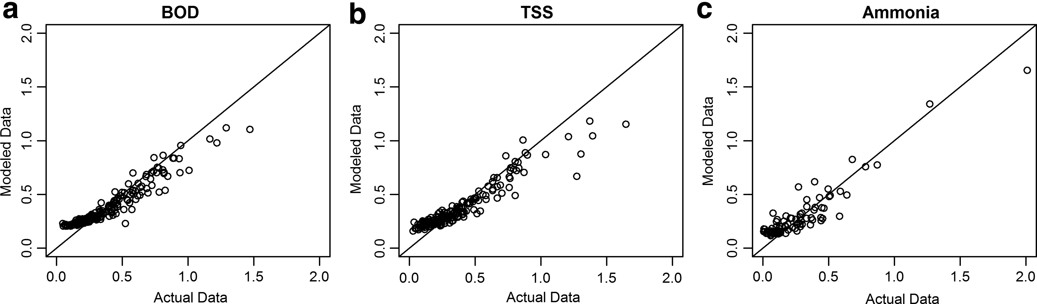
Modeled versus actual average relative effluent concentrations of (a) biological oxygen demand (BOD), (b) total suspended solids (TSS), and (c) ammonia for each facility, where relative effluent concentration is defined as the ratio of constituent effluent concentration to the permit limit.

Figure 2 shows the expected relative effluent concentration for three constituents for months after three representative relative effluent concentrations, R_t₋₁=0.5, 0.9, and 2.0, assuming a constant average flow rate. Expected effluent concentration is clearly correlated with the effluent level of the previous month. Furthermore, the models for BOD and TSS indicate that large and overloaded facilities can expect the highest effluent concentrations in the month after relative effluent concentrations of 0.9 (nonviolations); however, in the month after permit violations (R_t₋₁>1), small, overloaded facilities and large underloaded facilities are expected to have the highest effluent constituent concentrations. This trend is more pronounced for effluent TSS than for BOD. In contrast, small facilities, in general, have the highest expected effluent ammonia concentration in months after violations as well as in months where the effluent ammonia was close to but below the permit level (R_t₋₁=0.9). Lower resilience of ammonia removal for small plants is not surprising given the extra demands that biological nitrification processes place on facilities and operators.

FIG. 2.

Expected value of the relative effluent concentration for BOD, TSS, and ammonia from the Generalized Linear Model as a function of three values of the previous month's relative effluent concentration. R_t₋₁=2 indicates significant violation of permit value in the previous month.

As described earlier, the model predicts the expected effluent concentration under a Gamma distribution at each time step based on the expected effluent concentration and the associated standard errors. With the obtained Gamma distribution, the probability of an effluent concentration >1 can be calculated as the value of the cumulative distribution function evaluated at 1. This probability for BOD violation is obtained for all the observations and is shown as surfaces in Fig. 3. They mirror the patterns apparent for effluent concentration shown in Fig. 1. After a month with an effluent concentration half of the permitted level (R_t₋₁=0.5), the probability of a violation for BOD in the next month is low. In this situation, small and overloaded facilities had the highest probability of a subsequent violation, 12%. In contrast, after relative effluent levels of 90% of the permitted level or an actual violation, facilities of any size and capacity utilization can expect concentrations close to or greater than the permitted level with a 50% probability of a violation during the the next month, but small and overloaded facilities actually have the lowest probability of a violation. Finally, in the month after a permit violation (R_t₋₁=2), all facilities have at least a 50% probability of a violation the next month. In this situation, small facilities operating at over their permit capacity again perform the worst with the probability of a permit violation for BOD, TSS, or ammonia between 60% and 100%. Violation probability for TSS and ammonia, not shown, also follows the same patterns evident in effluent concentration. Specifically, TSS violation probability for small plants is more dependent on capacity utilization, and small overloaded facilities have a higher probability of an ammonia violation than other facilities for all values of R_t₋₁.

FIG. 3.

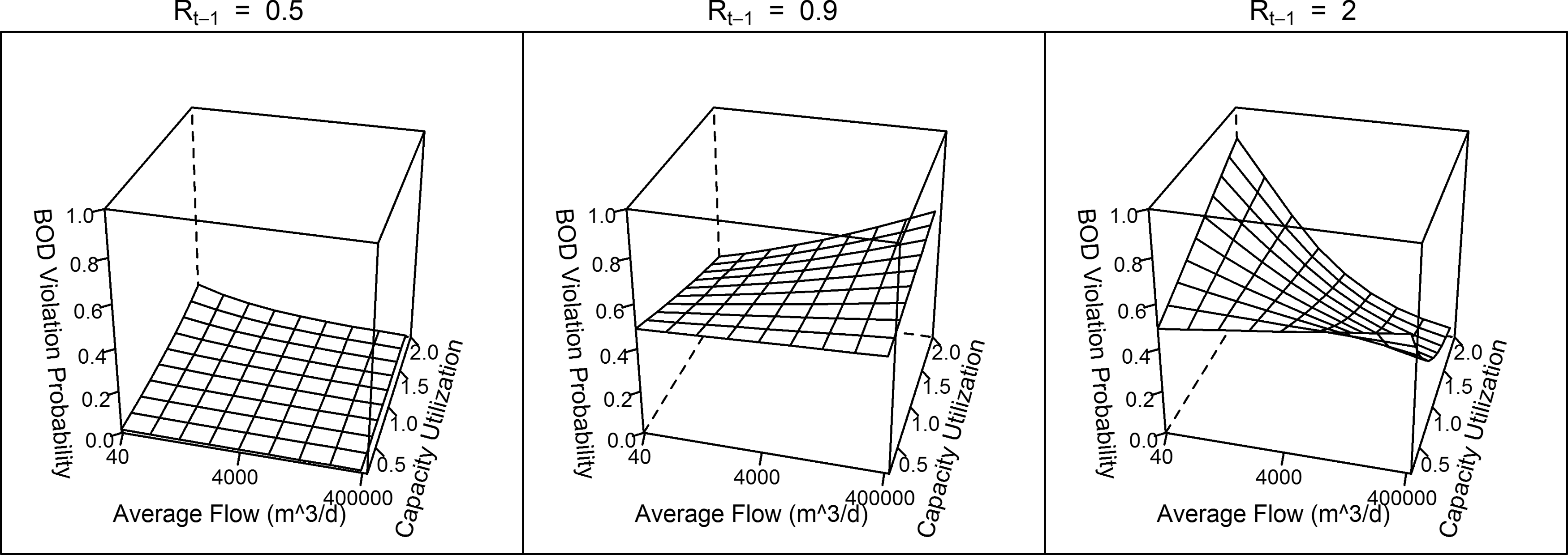
Probability of a permit violation for effluent BOD as a function of average flow and capacity utilization given three relative effluent concentrations in the previous month, where R_t₋₁=2 indicates a significant violation—effluent BOD of twice the permit limit.

Discussion

Biological oxygen demand

Figure 4a shows average violation length; Fig. 4b shows the number of separate violation sequences; Fig. 4c shows the average relative effluent; and Fig. 4d shows the fraction of months in violation, all of which are with regard to BOD. The model predicts that small and overloaded facilities have the highest average effluent levels, which coincide with large numbers of violation sequences per year. Specifically, facilities 40,000 m³/day (10.5 million gallons per day [MGD]) and larger can expect 0.1 violation per year, while facilities 400 m³/day (0.105 MGD) and smaller should expect violations proportional to their capacity utilization ranging from 0.1 per year for those significantly underloaded to 0.8 per year or more for those receiving flows significantly higher than their rated capacity. As expected, these results are consistent with those from the expected estimates of the fitted GLM shown in Fig. 3. Thus, instability, measured as total number of violations over the 10-year simulation period, corresponds strongly with violation probability after good treatment performance (R_t₋₁=0.5).

FIG. 4.

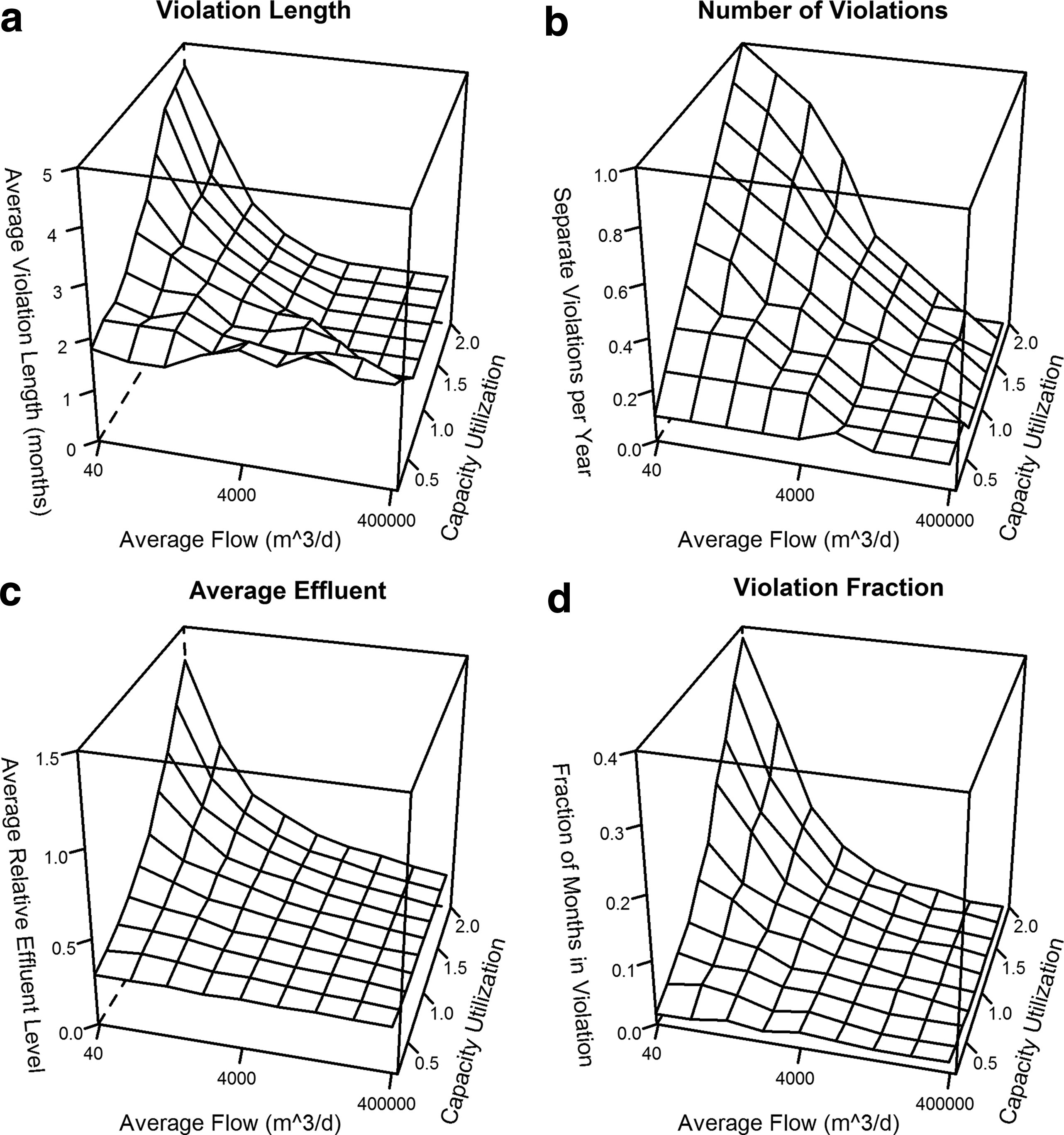
Long-term simulated resilience and stability of BOD removal for wastewater treatment facilities as determined by capacity and capacity utilization. Plots are median values of (a) simulated average violation length, (b) number of independent violations per year, (c) average relative effluent concentration, and (d) fraction of months in violation over the 10-year time series.

Average violation length has a similar trend: Small and overloaded facilities are the least resilient. BOD violation length was greater than 4 months long for these facilities, ∼3 months for large and underutilized facilities. For facilities receiving flows of 50% of their rated capacity (C_t=0.5), the expected average violation length ranged from 2 months for A_t<400 m³/day to 1.2 months for A_t>40,000 m³/day. Small overloaded facilities have the highest average relative effluent BOD concentration (M) and the highest fraction of months in violation (F) over the 10-year simulation, which is consistent with previous findings (Weirich et al., 2011).

Total suspended solids

Results from simulations of effluent TSS (Fig. 5) show different trends from those of BOD. First, average length of violation is 2 months for all facilities and does not vary significantly with flow rate or capacity utilization. Second, there are distinct trends in the number of separate violation sequences, as seen in Fig. 5c. Most striking is the large number of violation sequences for facilities that are both large and over-utilized. However, the significance of this prediction is minimal as all facilities larger than 10,000 m³/day had capacity utilization under 1.3, though smaller facilities had capacity utilization till 1.8. Thus, underloaded large facilities can expect nearly 0 violations per year, while those with capacity utilization of nearly 1.3 can expect 0.3 separate violations per year. It is expected that TSS removal would be sensitive to overloading regardless of facility size. Higher flows are associated with increased BOD loading and higher mixed liquor suspended solids, resulting in increased hydraulic and solids loading to the secondary clarifiers. However, capacity utilization is less of a factor for smaller facilities, such that 400 m³/day facilities can expect 0.3 violations per year regardless of utilization. Factors other than loading, such as algae growth in polishing ponds and excessive solid accumulation in the clarifiers due to infrequent disposal, may particularly affect solid discharge at small facilities.

FIG. 5.

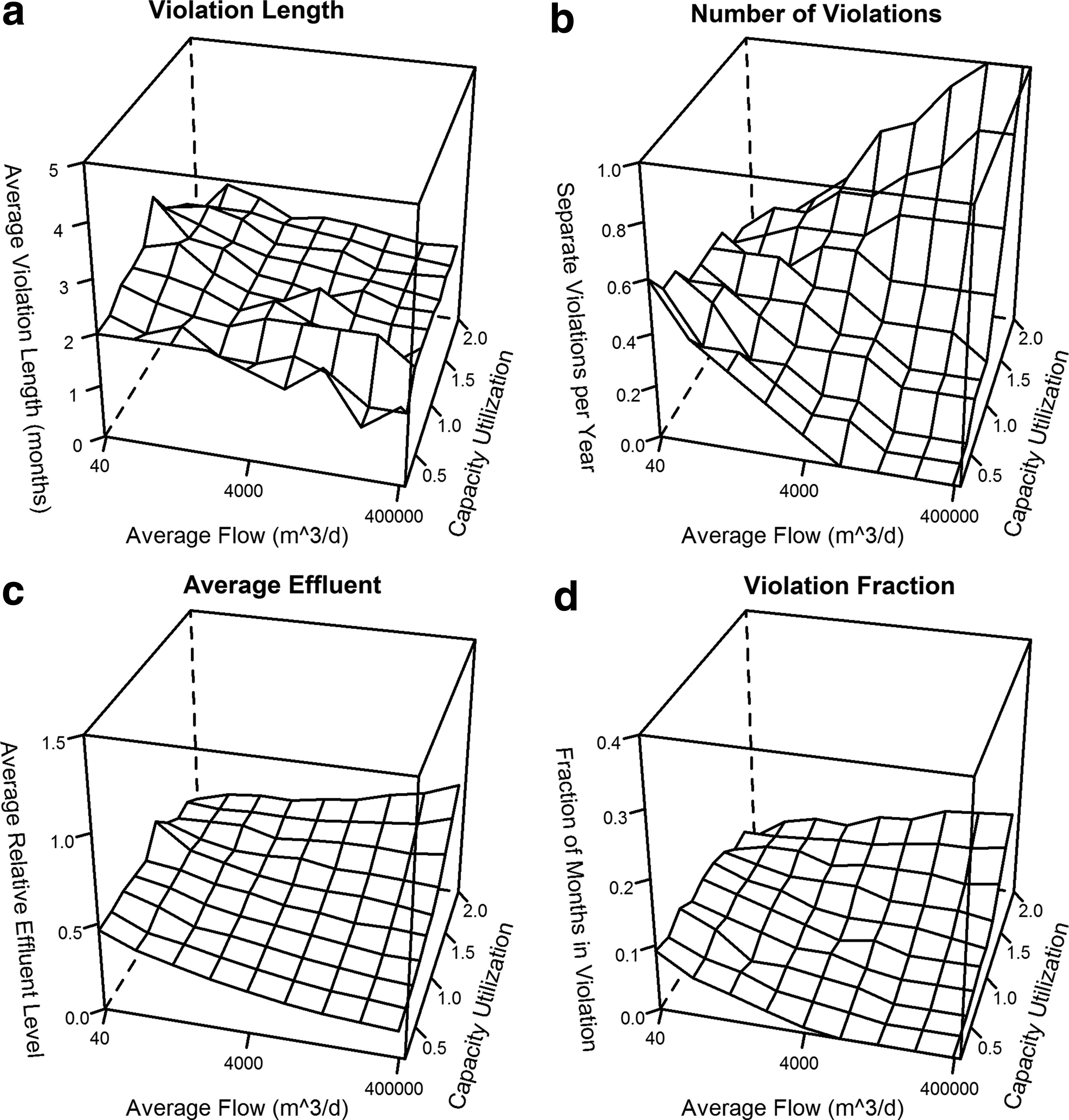
Long-term simulated resilience and stability of TSS removal for wastewater treatment facilities as determined by capacity and capacity utilization. Plots are median values of (a) simulated average violation length, (b) number of independent violations per year, (c) average relative effluent concentration, and (d) fraction of months in violation over the 10-year time series.

Predicted average relative effluent concentrations and violation fraction follow the same trends as the number of violations. Small underloaded facilities and large overloaded facilities average 0.5 times their permitted discharge with violations during 10% of months while other facilities average as low as 0.2 times their permit level and 1% violations.

Ammonia

Simulation results for effluent ammonia are shown in Fig. 6. The model predicts that on average most facilities discharge ∼30% of their permitted limit, but there is a sharp increase in predicted discharge concentration for facilities smaller than 400 m³/day treating flows over their design capacity. Violation fraction and average length of violation follow roughly the same pattern. Over the 10-year simulation, the median ammonia violation frequency is ∼5% and the average violation duration is 2 months, but small, overloaded facilities perform significantly worse on both measures, as shown in Fig. 6a and d. The simulated number of separate ammonia violations decreases as facility size increases. Facilities with an average flow of 400 m³/day average 0.2 separate violations per year, while those with a flow of 40,000 m³/day average only 0.1 violations per year. Unlike an earlier study on the probability of excess ammonia releases over a short duration (Weirich et al., 2011), capacity utilization is a significant factor in the overall fraction of months in violation over the 10-year time frame; however, the relationship is seen in the length of violations and not in the frequency of occurrence.

FIG. 6.

Long-term simulated resilience and stability of ammonia removal for wastewater treatment facilities as determined by capacity and capacity utilization. Plots are median values of (a) simulated average violation length, (b) number of independent violations per year, (c) average relative effluent concentration, and (d) fraction of months in violation over the 10-year time series.

Overall

The likelihood of a permit violation is significantly increased by a previous month's violation for BOD, TSS, and ammonia, across all plant capacities and hydraulic loading values. Moreover, given a BOD discharge violation in 1 month, the expected duration of subsequent violations varied from 2 to 5 months and small plants receiving higher than capacity flows (flow ≤400 m³/day, and capacity utilization >1) are predicted to have the longest duration of monthly violations. A similar trend was found for ammonia.

Another finding of this study is that small and overloaded plants are the least stable when considering BOD and ammonia removal. These facilities average one expected violation per year, several times more frequent than larger or underloaded facilities. Overloading can lead to reduced treatment performance through inadequate hydraulic residence times and increased loss of solids, both of which should affect plants of all sizes. In contrast, average flow and capacity utilization are unrelated to the time for plants to recover from TSS violations, and facilities across the range of capacity average ∼2 month-long TSS violation sequences. TSS violations at large overloaded facilities are expected more frequently than for smaller facilities.

Analysis using these models shows that the effluent concentrations of BOD and ammonia of small facilities are more sensitive to overloading than those of larger facilities. This fact suggests that these small facilities share underlying characteristics that affect their resilience and stability, including the inability to learn from past performance or to adapt to failures. The importance of overloading for small facilities also suggests that accurate growth forecasting and timely facility upgrades are needed even in small facilities. This is in contrast with other work which suggests that one main advantage of decentralized facilities is phased, as needed construction (Pinkham et al., 2004).

These models also revealed that the factors that affect TSS removal are different than those determining BOD and ammonia removal. Smaller facilities may have proportionally larger clarifiers or off-line storage for solids in ponds. The prevalence of extended air processes at smaller facilities may also provide more volume so that flows in excess of rated capacity are less significant than at larger plants. Also, longer aeration times may lead to decreased solid production.

Attempts to model the dependence of effluent fecal coliform concentration on the previous month's performance using the GLM method were not successful. Previous research has shown that facility capacity and loading were not good predictors of either relative effluent coliform density or violations, possibly due to the fact that disinfection is a different process than BOD, TSS, and ammonia removal (Weirich et al., 2011). Likely the inability of the GLM simulation to predict recovery from fecal coliform violations has the same explanation.

Conclusions

Resilience and stability of facilities such as wastewater treatment plants are important aspects of sustainability, and both are time-dependent properties. Thus, any models or simulations used to analyze these properties must also be time dependent. Resilience is defined as the ability for a system to recover from a perturbation or failure and is quantified in this study as the length of successive monthly violations of discharge standards. Stability is measured by the predicted frequency of violations over a time period. A statistical model has been developed to quantify resilience and stability by evaluating plant performance as a continuum with dependence on earlier performance rather than as independent monthly events, while still incorporating time-independent factors, namely average flow rate and capacity utilization.

An important potential application of the time series approach developed for this study is prediction of cumulative pollution risk to a receiving water or watershed. The authors suggest that one use of this model is for water use and urban planners to estimate the effects of future wastewater treatment on a receiving body without specific treatment characteristics. They could predict that the effects of decentralization and network topology could be investigating, including questions such as the effect of development density, different spatial distributions of treatment, and dilution by larger facilities. They could also plan for the economic costs of excess discharges of BOD, TSS, and ammonia, including regulatory penalties and lost revenue. Once the basic wastewater treatment plan has been established, the permit limits and desired effluent characteristics could be determined based on this model and the information it provides about the significance of violations. These limits would be passed to engineers using other resources such as BIOWIN to design and analyze specific treatment processes for implementation.

In this way, this model adds to the resources available for water managers by providing a means for a first-pass simulation of treatment performance without requiring the detail and expense of a more in-depth model. This model also provides valuable information of the likelihood and characteristics of permit violations, which fall outside the planned performance of facilities but are a significant contribution to surface water impairment.

Footnotes

Author Disclosure Statement

No competing financial interests exist.

References

Akaike

(1974). A new look at the statistical model identification. IEEE Trans. Autom. Control, 19, 716.

Centre for Alternative Wastewater Treatment. (2009). Available at: http://cawt.ca/about-us/objectives (accessed December 17, 2014).

Corotis

R.B.

(2011). Conceptual and analytical differences between resiliency and reliability for seismic hazards. Presented at Structures Congress 2011, Las Vegas, NV, April 14–16.

Fane

S.A.

, Willetts

, Abeysuriya

, Mitchell

, Etnier

, and Johnstone

(2004). Evaluating reliability and life-cycle cost for decentralised wastewater within the context of asset management. Presented at the 6th Specialist Conference on Small Water and Wastewater Systems and 1st International Conference on Onsite Wastewater Treatment and Recycling. Fremantle, Australia, February 11–13.

Furrer

E.M.

, and Katz

R.W.

(2007). Generalized linear modeling approach to stochastic weather generators. Clim. Res., 34, 129.

Hao

R.X.

, Li

S.M.

, Li

J.B.

, Zhang

Q.K.

, and Liu

(2013). Water quality assessment for wastewater reclamation using principal component analysis. J. Environ. Inform., 21, 45.

McCullagh

, and Nelder

J.A.

(1989). Generalized Linear Models. London: Chapman and Hall.

McDaniels

, Chang

, Cole

, Mikawoz

, and Longstaff

(2008). Fostering resilience to extreme events within infrastructure systems: Characterizing decision contexts for mitigation and adaptation. Bus. Soc., 18, 310.

National Decentralized Water Resources Capacity Development Project. (2009). Available at: www.ndwrcdp.org/ (accessed June 1, 2009).

10.

National Environmental Services Center. (2008). Wastewater and Onsite Systems Programs. Available at: www.nesc.wvu.edu/wastewater.cfm (accessed January 20, 2009).

11.

Niku

, and Schroeder

E.D.

(1979). Performance of activated sludge process and reliability-based design. J. Water Pollut. Control Fed., 51, 2841.

12.

Niku

, and Schroeder

E.D.

(1981) Factors affecting effluent variability from activated sludge processes. J. Water Pollut. Control Fed, 53, 546.

13.

Oakley

S.M.

, Gold

A.J.

, and Oczkowski

A.J.

(2010). Nitrogen control through decentralized wastewater treatment: Process performance and alternative management strategies. Ecol. Eng., 36, 1520.

14.

Oliveira

S.C.

, and Von Sperling

(2008). Reliability analysis of wastewater treatment plants. Water Res., 42, 1182.

15.

Pinkham

R.D.

, Magliaro

, and Kinsley

(2004). Case Studies of Economic Analysis and Community Decision making for Decentralized Wastewater Systems. Project No. WU-HT-02-03. Prepared for the National Decentralized Water Resources Capacity Development Project, Washington University, St. Louis, MO, by Rocky Mountain Institute, Snowmass, CO.

16.

U.S. Environmental Protection Agency. (1997). Response to Congress on Use of Decentralized Wastewater Treatment Systems. EPA 832-R-97-001b. Washington, D.C.: Office of Wastewater Management.

17.

U.S. Environmental Protection Agency. (2002). The Clean Water and Drinking Water Infrastructure Gap Analysis. EPA-816-R-02-020. Available at: www.epa.gov/ogwdw/gapreport.pdf (accessed December 17, 2014).

18.

U.S. Environmental Protection Agency. (2008a). 2004 Clean Watersheds Needs Survey: Report to Congress. Available at: http://water.epa.gov/scitech/datait/databases/cwns/upload/cwns2008rtc.pdf (accessed February 12, 2009).

19.

U.S. Environmental Protection Agency. (2008b). Enforcement and Compliance History Online (ECHO). Available at: http://echo.epa.gov/ (accessed January 14, 2010).

20.

U.S. Environmental Protection Agency. (2008c). Gulf Hypoxia Action Plan. Available at: http://water.epa.gov/type/watersheds/named/msbasin/upload/2008_8_28_msbasin_ghap2008_update082608.pdf (accessed February 12, 2009).

21.

U.S. Environmental Protection Agency. (2009). National Water Quality Inventory: Report to Congress. EPA 841-R-08-001. Available at: http://water.epa.gov/lawsregs/guidance/cwa/305b/upload/2009_01_22_305b_2004report_2004_305Breport.pdf (accessed December 17, 2014).

22.

Weirich

S.R.

, Silverstein

, and Rajagopalan

(2011). Effect of average flow and capacity utilization on effluent water quality from US municipal wastewater treatment facilities. Water Res., 45, 4279.