Clogging Simulation of Horizontal Subsurface-Flow Constructed Wetland

Abstract

Clogging of constructed wetlands commonly occurs; however, clogging of horizontal subsurface-flow constructed wetlands (HSSFCW) has not been successfully simulated using mathematical models. This study established a mathematical model by coupling one-dimensional mass transfer model with multicomponent biochemical reactions by using Constructed Wetland Model No. 1 to simulate clogging during treatment of domestic sewage with HSSFCW. Complex relations among porosity, hydraulic conductivity, and retention capability of particles were dodged dexterously in the new model by using total particle concentration within interstitial space as indicator of clogging. Introducing particulate component release ratio, which controlled the transmission of particles within substrates, and using substrate porosity as constant simplified the simulation and saved computation time. Clogging degree can be easily identified by comparing total particle concentration in the interstitial space with the concentration threshold of clogging, such as biofilm density. The value of particulate component release ratio was determined, and the model was calibrated using measured data from the literature. Results showed that the proposed model can successfully simulate clogging and explain the underlying mechanism of HSSFCW. The new model supplied a simple method for predicting the clogging of HSSFCW.

Introduction

Subsurface-flow constructed wetland (SFCW) is a type of ecological wastewater treatment that emerged in 1970 s; this treatment uses substrates, aquatic plants, and microorganisms with physical, chemical, and biological reactions to purify wastewater. SFCW is widely used in sewage treatment in small towns and rural areas because of its low capital investment, low running costs, simple maintenance and management, and good treatment effects; SFCW has become one of the most important techniques for water pollution control in the last decade (Winter and Goetz, 2003; Kadlec and Wallace, 2009).

Clogging frequently occurs when SFCW operate for long periods of time. The longevity of SFCW is estimated to be 15 (Cooper et al., 1996) and 10 years (Wallace and Knight, 2006), whereas Griffin et al. (2008) reckoned that the service life of SFCW would be approximately 8 years. According to more than 100 running wetland surveys of the EPA, approximately half of the constructed wetlands are clogged within 5 years after use (USEPA, 1993). Consequently, the clogging of SFCW has become one of the key points in sewage treatment.

Substrate clogging in SFCW is caused by several physical, chemical, and biological factors (Platzer and Mauch, 1997; Langergraber et al., 2004). In terms of physical factors, the inflow of a large number of suspended solids (especially nonbiodegradable solids) into the wetland and reduced porosity are the main causes of clogging (Blazejewski and Murat–Blazejewska, 1997; Zhao, et al., 2004). The interception, deposition, and other physical and chemical processes induce the removal of organic matter and total particulates near the inlet area (Pedescoll et al., 2009). Wetlands accumulate humus and extracellular polymeric substances secreted by some bacteria, resulting in the formation of glutinous sludge with high water content and low density, and inducing wetland clogging (Winter and Goetz, 2003). Therefore, clogging in SFCW is a complicated process affected by several factors. As a consequence, mathematical models that can successfully simulate clogging processes are rare, especially for horizontal subsurface-flow constructed wetlands (HSSFCW).

The main mathematical models reported are the following:

(1) Blazejewski and Murat–Blazejewska (1997) proposed a simple algebraic expression to estimate clogging by calculating the time of inflow suspended solids filling up the porosity of clogging layer, which is effective in modeling vertical subsurface-flow constructed wetlands (VSSFCW) in laboratory scale (Boller and Kavanaugh, 1995; Hua et al., 2010).

(2) Exponential relationship between the loss of permeability coefficient and cumulative solid load was used to describe wetland clogging (Platzer and Mauch, 1997; Hyánková et al., 2006).

(3) Based on Carman–Kozeny's (C-K) equation, a temporal and spatial model was used to simulate the development of spatially varying permeability coefficient during clogging process, as well as the relationship between solid accumulation and decrease in permeability coefficient (Knowles and Davies, 2011). However, the calculated permeability coefficient was less compared with the measured value because of the neglected clogging from other sources, such as biological and chemical effects (Knowles and Davies, 2011; Nivalaet al., 2012).

(4) A complex model named FITOVERT was developed by Giraldi et al. (2010) to simulate the cumulative behavior of biofilm and particulate substances in one-dimensional VSSFCW. FITOVERT combines the hydraulic module, biochemical module, and transport equation of dissolved and particulate components. The infiltration coefficient is embedded into a convective mass transport equation. The porosity of substrates and permeability coefficients is considered using the C-K equation. The treatment process for biodegradable organic carbon and nitrogen is described following Activated Sludge Model 1 (ASM1). FITOVERT neglects the diffusion of dissolved components within the biofilm, as well as the role of the plant absorption of nutrients. However, only the hydraulic module has been calibrated and validated, and the biochemical reaction term of particulate components is not included in the conservation equation. The latter is not consistent with the practice that the main biodegradable components in sewage are treated as particles. Therefore, this complex model is still at the development stage and is far from being implemented at a practical level (Nivala et al., 2012).

For simple and reasonable simulation of clogging in treating domestic sewage with HSSFCW, this article proposed a mathematical model by coupling one-dimensional mass transfer model with multicomponent biochemical reaction based on Constructed Wetland Model No. 1 (CWM1) (Langergraber et al., 2009). Complex relationships among porosity, hydraulic conductivity, and retention capability of particles were dodged dexterously in the new model by using total particle concentration within interstitial space as indicator of clogging. Release rate was introduced and designated as the key parameter for controlling the transmission of the particulate components. The computational unit size of wetlands in the model was determined using an empirical formula of the clogging layer thickness of particle state substance. The model was calibrated using measured data from the literature (Llorens et al., 2009). This study aimed to develop a simple and reasonable method for simulating clogging in HSSFCW.

Model Establishment

Modeling ideas

Simulation steps of the constructed wetland clogging model included the following:

(1) Input water quality parameter value;

(2) input parameter values of constructed wetlands;

(3) determine the values of retention parameters of the substrate (such as interception coefficient or release coefficient) and parameters of microbial kinetics;

(4) solve the mass conservation equations, including mass transfer and microbial degradation, and obtain the distribution of the concentration of particulate matter in the substrate;

(5) determine substrate porosity reduced by the concentration of particulate matter and its density;

(6) repeat steps (4) and (5) with the new value of porosity; and

(7) calculate the hydraulic conductivity coefficient with the reduction of porosity and evaluate the clogging degree of the wetland with the reduction of hydraulic conductivity coefficient.

These procedures require the calculation of the reduction in substrate porosity repeatedly and are thus time-consuming. Moreover, the results of the calculated porosity have considerable deviation with the actual one. Therefore, this study considered using the following procedures to simulate wetland clogging.

(1) to (4) is the same as those mentioned previously;

(5) use the initial porosity of the substrate to repeat step (4) and obtain the temporal and spatial distribution of particulate matter;

(6) determine the degree of wetland clogging by comparing total particulate matter concentration with the threshold of blocking concentration.

Development of one-dimensional mass transfer model

The substrates in wetlands are supposed to be homogeneous along the horizontal and vertical direction. Along its length, the wetland was divided into n small units (computational grids), in which the mass concentration of various components was equal. Supposedly, the flow rate in each unit was not variable, but equal to the inflow rate of the HSSFCW. The boundary of each unit was assumed to intercept particulate component X_i, but the same cannot occur for dissolved component S_i. Ignoring the effect of reduced water levels on flow cross-section, one-dimensional and partial differential equations of component X_i in the jth unit of the wetland could be written as follows based on mass conservation equation: \documentclass{aastex}\usepackage{amsbsy}\usepackage{amsfonts}\usepackage{amssymb}\usepackage{bm}\usepackage{mathrsfs}\usepackage{pifont}\usepackage{stmaryrd}\usepackage{textcomp}\usepackage{portland, xspace}\usepackage{amsmath, amsxtra}\pagestyle{empty}\DeclareMathSizes{10}{9}{7}{6}\begin{document} \begin{align*} { \frac { \partial { X_ { { \rm { i , j } } } } } { \partial t } } = { \frac { \partial ( { u_ { { \rm { x , j } } } } { X_ { { \rm { i , j } } } } ) } { \partial x } } + { r_ { { \rm { i , j } } } } \tag { 1 } \end{align*} \end{document}

where X_i,j [mg/L] = concentration of the ith kind particulate component in unit j; j = 1, 2, 3…n; n = the number of units; u_x,j [m/s] = the flow velocity along the length of wetlands in unit j; r_i,j [mg/(L·s)] = reaction rate of the ith kind particulate component in unit j; x [m] = coordinate along the length of the wetland; and t [s] = operation time for wetland.

Particulate release ratio (R_j) in unit j is introduced and defined in Equation (2): \documentclass{aastex}\usepackage{amsbsy}\usepackage{amsfonts}\usepackage{amssymb}\usepackage{bm}\usepackage{mathrsfs}\usepackage{pifont}\usepackage{stmaryrd}\usepackage{textcomp}\usepackage{portland, xspace}\usepackage{amsmath, amsxtra}\pagestyle{empty}\DeclareMathSizes{10}{9}{7}{6}\begin{document} \begin{align*} {R_{ \rm{j}}} = \mathop \sum \limits_{{ \rm{i}} = { \rm{1}}} {{X_{{ \rm{i ( e ), j}}}}} / \mathop \sum \limits_{{ \rm{i}} = { \rm{1}}} {{X_{{ \rm{i , j}}}}} \tag{2} \end{align*} \end{document}

where X_i(e),j [mg/L] = concentration of particulate component i effluent from unit j, and R_j [−] = the average release ratio of particulates in unit j.

Concentration of particulates i in the effluent from unit j could be approximated as follows: \documentclass{aastex}\usepackage{amsbsy}\usepackage{amsfonts}\usepackage{amssymb}\usepackage{bm}\usepackage{mathrsfs}\usepackage{pifont}\usepackage{stmaryrd}\usepackage{textcomp}\usepackage{portland, xspace}\usepackage{amsmath, amsxtra}\pagestyle{empty}\DeclareMathSizes{10}{9}{7}{6}\begin{document} \begin{align*} {X_{{ \rm{i ( e ), j}}}} = {R_{ \rm{j}}} \cdot {X_{{ \rm{i , j}}}} \tag{3} \end{align*} \end{document}

The particulate release ratio R_j is a variable and varies with substrate porosity ( \documentclass{aastex}\usepackage{amsbsy}\usepackage{amsfonts}\usepackage{amssymb}\usepackage{bm}\usepackage{mathrsfs}\usepackage{pifont}\usepackage{stmaryrd}\usepackage{textcomp}\usepackage{portland, xspace}\usepackage{amsmath, amsxtra}\pagestyle{empty}\DeclareMathSizes{10}{9}{7}{6}\begin{document} $${ \varepsilon _{ \rm{j}}}$$ \end{document} ). For example, when the substrate porosity is equal to zero, no particulates can be transmitted to the next unit and R_j should be equal to zero. However, in actual practice of HSSFCW, particulates can be transmitted to the next substrate unit with fluids through overflow when one substrate unit is clogged. This phenomenon is a major difference between HSSFCW and VSSFCW. Therefore, to simulate the actual transmission of particulates through overflow in HSSFCW, we used R_j as constant in the model for all computational units.

Equation (2) shows that if biodegradation is ignored, the effluent particle concentration in the first substrate unit can follow that of the influent when the particle concentration within the substrate unit accumulates to a substantial value. This assumption implies that Equation (3) with a constant R_j can represent the actual situation of influent autoreturning to the next unit through overflow when the first unit is clogged. As a consequence, using R_j as a constant may reflect the actual situations when clogging occurs in the front unit.

Factors such as diameter, shape, and porosity of substrate, as well as length of computational unit may influence the value of R_j. In this study, the value of R_j was determined as 0.0043 through model calibration.

Porosity could be related to the ratio of total particulate component concentration and to the greatest average density of solids accumulated in the substrate of one computational unit. Hence, we used biofilm density, instead of the highest density of solids, as follows: \documentclass{aastex}\usepackage{amsbsy}\usepackage{amsfonts}\usepackage{amssymb}\usepackage{bm}\usepackage{mathrsfs}\usepackage{pifont}\usepackage{stmaryrd}\usepackage{textcomp}\usepackage{portland, xspace}\usepackage{amsmath, amsxtra}\pagestyle{empty}\DeclareMathSizes{10}{9}{7}{6}\begin{document} \begin{align*} { \varepsilon _{ \rm{j}}} = { \varepsilon _0} ( 1 - \mathop \sum \limits_{{ \rm{i}} = 1} {{X_{{ \rm{i , j}}}}} / { \rho _{ \rm{b}}} ). \tag{4} \end{align*} \end{document}

Porosity of unit j \documentclass{aastex}\usepackage{amsbsy}\usepackage{amsfonts}\usepackage{amssymb}\usepackage{bm}\usepackage{mathrsfs}\usepackage{pifont}\usepackage{stmaryrd}\usepackage{textcomp}\usepackage{portland, xspace}\usepackage{amsmath, amsxtra}\pagestyle{empty}\DeclareMathSizes{10}{9}{7}{6}\begin{document} $${ \varepsilon _{ \rm{j}}}$$ \end{document} was employed as a variable in some clogging models reported (Giraldi et al., 2010). However, we set \documentclass{aastex}\usepackage{amsbsy}\usepackage{amsfonts}\usepackage{amssymb}\usepackage{bm}\usepackage{mathrsfs}\usepackage{pifont}\usepackage{stmaryrd}\usepackage{textcomp}\usepackage{portland, xspace}\usepackage{amsmath, amsxtra}\pagestyle{empty}\DeclareMathSizes{10}{9}{7}{6}\begin{document} $${ \varepsilon _{ \rm{j}}}$$ \end{document} as equal to the initial porosity value ( \documentclass{aastex}\usepackage{amsbsy}\usepackage{amsfonts}\usepackage{amssymb}\usepackage{bm}\usepackage{mathrsfs}\usepackage{pifont}\usepackage{stmaryrd}\usepackage{textcomp}\usepackage{portland, xspace}\usepackage{amsmath, amsxtra}\pagestyle{empty}\DeclareMathSizes{10}{9}{7}{6}\begin{document} $${ \varepsilon _0}$$ \end{document} ) in this study. Taking \documentclass{aastex}\usepackage{amsbsy}\usepackage{amsfonts}\usepackage{amssymb}\usepackage{bm}\usepackage{mathrsfs}\usepackage{pifont}\usepackage{stmaryrd}\usepackage{textcomp}\usepackage{portland, xspace}\usepackage{amsmath, amsxtra}\pagestyle{empty}\DeclareMathSizes{10}{9}{7}{6}\begin{document} $${ \varepsilon _{ \rm{j}}}$$ \end{document} as a constant for all computational units could not only save computational time but also represent the actual situation. We aim to calculate the total particle concentration X_i,j in the interstitial space (the initial interstitial space, but not the decreased interstitial void space) of the substrate of one computational unit, as shown in Fig. 1. X_i,j should be calculated with \documentclass{aastex}\usepackage{amsbsy}\usepackage{amsfonts}\usepackage{amssymb}\usepackage{bm}\usepackage{mathrsfs}\usepackage{pifont}\usepackage{stmaryrd}\usepackage{textcomp}\usepackage{portland, xspace}\usepackage{amsmath, amsxtra}\pagestyle{empty}\DeclareMathSizes{10}{9}{7}{6}\begin{document} $${ \varepsilon _0}$$ \end{document} as follows: \documentclass{aastex}\usepackage{amsbsy}\usepackage{amsfonts}\usepackage{amssymb}\usepackage{bm}\usepackage{mathrsfs}\usepackage{pifont}\usepackage{stmaryrd}\usepackage{textcomp}\usepackage{portland, xspace}\usepackage{amsmath, amsxtra}\pagestyle{empty}\DeclareMathSizes{10}{9}{7}{6}\begin{document} \begin{align*} {X_{\rm i , j}} = {V_{\rm b}} \cdot{ \rho _{\rm b}} / \left( {{V_{\rm j}} - {V_{\rm s}}} \right) { \rm{ }} = {V_{\rm b}} \cdot{ \rho _{\rm b}} / ( { \varepsilon _0} \cdot{V_{\rm j}} ) \tag{5} \end{align*} \end{document}

FIG. 1.

Modeling principle diagram. X_i,j = concentration of the ith kind particulate component in unit j; X_i(in),j = concentration of particulate component i in influent of unit j; R_j = release ratio; Q = inflow rate; ρ_b = biofilm density; ɛ₀ = initial porosity; V_b = volume of particulate matter or bioflim; V_s = volume of substrate; V_j = volume of computational unit.

where V_b [m³] = volume of particulate matter or biofilm; V_s [m³] = volume of substrate; V_j [m³] = volume of computational unit; and \documentclass{aastex}\usepackage{amsbsy}\usepackage{amsfonts}\usepackage{amssymb}\usepackage{bm}\usepackage{mathrsfs}\usepackage{pifont}\usepackage{stmaryrd}\usepackage{textcomp}\usepackage{portland, xspace}\usepackage{amsmath, amsxtra}\pagestyle{empty}\DeclareMathSizes{10}{9}{7}{6}\begin{document} $${ \varepsilon _0}$$ \end{document} [−] = the initial porosity value.

Thus, the one-dimensional mass transfer equation should be written as follows: \documentclass{aastex}\usepackage{amsbsy}\usepackage{amsfonts}\usepackage{amssymb}\usepackage{bm}\usepackage{mathrsfs}\usepackage{pifont}\usepackage{stmaryrd}\usepackage{textcomp}\usepackage{portland, xspace}\usepackage{amsmath, amsxtra}\pagestyle{empty}\DeclareMathSizes{10}{9}{7}{6}\begin{document} \begin{align*} { \frac { \partial { X_ { { \rm { i , j } } } } } { \partial t } } { \varepsilon _0 } { V_ { \rm { j } } } = Q ( { X_ { { \rm { i ( in ), j } } } } - { R_ { \rm { j } } } { X_ { { \rm { i , j } } } } ) \tag { 6 } \end{align*} \end{document}

A reasonable unit length is necessary so that indices in one unit are approximately homogeneous. Assuming that the growth rate of biomass is equal to the biodegradation rate of suspended solids, Blazejewski and Murat–Blazejewska (1997) developed a simple theoretical model for predicting clogging time t_c: \documentclass{aastex}\usepackage{amsbsy}\usepackage{amsfonts}\usepackage{amssymb}\usepackage{bm}\usepackage{mathrsfs}\usepackage{pifont}\usepackage{stmaryrd}\usepackage{textcomp}\usepackage{portland, xspace}\usepackage{amsmath, amsxtra}\pagestyle{empty}\DeclareMathSizes{10}{9}{7}{6}\begin{document} \begin{align*} {t_{ \rm{c}}} = 150{ \varepsilon _0}{ \rho _{ \rm{s}}} ( 1 - {w_{ \rm{c}}} ) {d_{{ \rm{ef}}}} / {q_{ \rm{s}}} \tag{7} \end{align*} \end{document}

and media porosity in wetland at time t was (Blazejewski and Murat–Blazejewska, 1997) as follows: \documentclass{aastex}\usepackage{amsbsy}\usepackage{amsfonts}\usepackage{amssymb}\usepackage{bm}\usepackage{mathrsfs}\usepackage{pifont}\usepackage{stmaryrd}\usepackage{textcomp}\usepackage{portland, xspace}\usepackage{amsmath, amsxtra}\pagestyle{empty}\DeclareMathSizes{10}{9}{7}{6}\begin{document} \begin{align*} { \varepsilon _{ \rm{t}}} = { \varepsilon _{ \rm{0}}} - {q_{ \rm{s}}}t / [ 150{ \rho _{ \rm{s}}} ( 1 - {w_{ \rm{c}}} ) {d_{{ \rm{ef}}}} ] \tag{8} \end{align*} \end{document}

Referring to Formulas (7) and (8) and supposing that the maximum unit length is 150 × d_ef, the minimum number of differential units could be determined using the following: \documentclass{aastex}\usepackage{amsbsy}\usepackage{amsfonts}\usepackage{amssymb}\usepackage{bm}\usepackage{mathrsfs}\usepackage{pifont}\usepackage{stmaryrd}\usepackage{textcomp}\usepackage{portland, xspace}\usepackage{amsmath, amsxtra}\pagestyle{empty}\DeclareMathSizes{10}{9}{7}{6}\begin{document} \begin{align*} n = L / ( 150 \cdot{d_{\rm ef}} ) \tag{9} \end{align*} \end{document}

where L [m] = length of wetland.

The length of computational unit is an important parameter because it is related to the value of release ratio.

Use of CWM1 model

Organic decomposition in wetlands is a biochemical reaction related to multicomponents and multipopulations. Hence, the CWM1 model was used in this study to describe the biochemical reaction. Langergraber et al. (2009) proposed CWM1 for describing biological conversion and degradation of organic matter, nitrogen, and sulfur with biokinetics of microorganisms in SSFCW. CWM1 mainly aims to predict effluent concentrations from the wetland. Matrix presentation, 17 biochemical processes, and 16 components (eight soluble and eight particulate) were introduced in CWM1. The 16 components and 17 biochemical processes are shown in Tables 1 and 2, respectively.

Table 1.

Components Used in Constructed Wetland Model No. 1

Number	Symbol	Components name
1	S_O	Dissolved oxygen
2	S_F	Fermentable, readily biodegradable soluble COD
3	S_A	Fermentation products as acetate
4	S_I	Inert soluble COD
5	S_NH	Ammonium and ammonia nitrogen
6	S_NO	Nitrate and nitrite nitrogen
7	S_SO4	Sulfatesulfur
8	S_H2S	Dihydrogensulfide sulfur
9	X_S	Slowly biodegradable particulate COD
10	X_I	Inert particulate COD
11	X_H	Heterotrophic bacteria
12	X_A	Autotrophic nitrifying bacteria
13	X_FB	Fermenting bacteria
14	X_AMB	Acetotrophic methanogenic bacteria
15	X_ASRB	Acetotrophic sulfate reducing bacteria
16	X_SOB	Sulfide oxidizing bacteria

Table 2.

Biochemical Processes Used in Constructed Wetland Model No. 1

Number	Name of biochemical processes
1	Hydrolysis
2	Aerobic growth of X_H on S_F
3	Aerobic growth X_H of on S_A
4	Anoxic growth of X_H on S_F
5	Anoxic growth of X_H on S_A
6	Lysis of X_H
7	Aerobic growth of X_A on S_NH
8	Lysis of X_A
9	Growth of X_FB
10	Lysis of X_FB
11	Growth of X_AMB
12	Lysis of X_AMB
13	Growth of X_ASRB
14	Lysis of X_ASRB
15	Aerobic growth of X_SOB on S_H2S
16	Anoxic growth of X_SOB on S_H2S
17	Lysis of X_SOB

CWM1 describes aerobic, anoxic, and anaerobic processes and is thus applicable to both horizontal and vertical flow CW systems. The kinetic rate expressions, values of kinetic parameters, and stoichiometric coefficients used in this article are referred to the study of Langergraber et al. (2009).

Coupling of one-dimensional mass transfer model with CWM1 model

Based on the observations, V and Q were assumed to represent the volume of wetland and influent flow, respectively, and the one-dimensional mass transfer model was combined with the CWM1 model. Equation (1) can be rewritten to express the mass conservation in unit j of particulate component X_i,j, dissolved component S_i,j, and dissolved oxygen DO_j. \documentclass{aastex}\usepackage{amsbsy}\usepackage{amsfonts}\usepackage{amssymb}\usepackage{bm}\usepackage{mathrsfs}\usepackage{pifont}\usepackage{stmaryrd}\usepackage{textcomp}\usepackage{portland, xspace}\usepackage{amsmath, amsxtra}\pagestyle{empty}\DeclareMathSizes{10}{9}{7}{6}\begin{document} \begin{align*} { \frac { \partial { X_ { { \rm { i , j } } } } } { \partial t } } = { \frac { n \cdot Q \cdot ( { X_ { { \rm { i ( in ), j } } } } - R \cdot { X_ { { \rm { i , j } } } } ) } { { \varepsilon _ { \rm { 0 } } } \cdot V } } + { r_ { { \rm { Xi , j } } } } \tag { 10 } \end{align*} \end{document} \documentclass{aastex}\usepackage{amsbsy}\usepackage{amsfonts}\usepackage{amssymb}\usepackage{bm}\usepackage{mathrsfs}\usepackage{pifont}\usepackage{stmaryrd}\usepackage{textcomp}\usepackage{portland, xspace}\usepackage{amsmath, amsxtra}\pagestyle{empty}\DeclareMathSizes{10}{9}{7}{6}\begin{document} \begin{align*} { \frac { \partial { S_ { { \rm { i , j } } } } } { \partial t } } = { \frac { n \cdot Q \cdot ( { S_ { { \rm { i ( in ), j } } } } - { S_ { { \rm { i , j } } } } ) } { { \varepsilon _ { \rm { 0 } } } \cdot V } } + { r_ { { \rm { Si , j } } } } \tag { 11 } \end{align*} \end{document} \documentclass{aastex}\usepackage{amsbsy}\usepackage{amsfonts}\usepackage{amssymb}\usepackage{bm}\usepackage{mathrsfs}\usepackage{pifont}\usepackage{stmaryrd}\usepackage{textcomp}\usepackage{portland, xspace}\usepackage{amsmath, amsxtra}\pagestyle{empty}\DeclareMathSizes{10}{9}{7}{6}\begin{document} \begin{align*} \frac { \partial DO} { \partial t} & = \frac {n \cdot Q \cdot ( DO_{ \rm{in , j}} - DO_{ \rm{j}}} { \varepsilon _{ \rm{0}} \cdot V }+ {K_{{ \rm{ls}}}} ( DO_{ \rm{s}} - DO_{ \rm{j}} ) \\& + {K_{\rm{lp}}}\frac {t } {K_{ \rm{lps}} + t }( DO_{ \rm{ps}} - DO_{ \rm{j}} ) + {r_{\rm{DO}}}_{ \rm{j}} \tag{12}\end{align*} \end{document}

where \documentclass{aastex}\usepackage{amsbsy}\usepackage{amsfonts}\usepackage{amssymb}\usepackage{bm}\usepackage{mathrsfs}\usepackage{pifont}\usepackage{stmaryrd}\usepackage{textcomp}\usepackage{portland, xspace}\usepackage{amsmath, amsxtra}\pagestyle{empty}\DeclareMathSizes{10}{9}{7}{6}\begin{document} $${X_{{ \rm{i ( in ), j}}}}$$ \end{document} , \documentclass{aastex}\usepackage{amsbsy}\usepackage{amsfonts}\usepackage{amssymb}\usepackage{bm}\usepackage{mathrsfs}\usepackage{pifont}\usepackage{stmaryrd}\usepackage{textcomp}\usepackage{portland, xspace}\usepackage{amsmath, amsxtra}\pagestyle{empty}\DeclareMathSizes{10}{9}{7}{6}\begin{document} $${X_{{ \rm{i , j}}}}$$ \end{document} [mg/L] = the concentration of particulate component i inflow and within unit j, respectively; \documentclass{aastex}\usepackage{amsbsy}\usepackage{amsfonts}\usepackage{amssymb}\usepackage{bm}\usepackage{mathrsfs}\usepackage{pifont}\usepackage{stmaryrd}\usepackage{textcomp}\usepackage{portland, xspace}\usepackage{amsmath, amsxtra}\pagestyle{empty}\DeclareMathSizes{10}{9}{7}{6}\begin{document} $${S_{{ \rm{i ( in ), j}}}}$$ \end{document} , \documentclass{aastex}\usepackage{amsbsy}\usepackage{amsfonts}\usepackage{amssymb}\usepackage{bm}\usepackage{mathrsfs}\usepackage{pifont}\usepackage{stmaryrd}\usepackage{textcomp}\usepackage{portland, xspace}\usepackage{amsmath, amsxtra}\pagestyle{empty}\DeclareMathSizes{10}{9}{7}{6}\begin{document} $${S_{{ \rm{i , j}}}}$$ \end{document} [mg/L] = the concentration of dissolved component i inflow and within unit j, respectively; \documentclass{aastex}\usepackage{amsbsy}\usepackage{amsfonts}\usepackage{amssymb}\usepackage{bm}\usepackage{mathrsfs}\usepackage{pifont}\usepackage{stmaryrd}\usepackage{textcomp}\usepackage{portland, xspace}\usepackage{amsmath, amsxtra}\pagestyle{empty}\DeclareMathSizes{10}{9}{7}{6}\begin{document} $$D{O_{{ \rm{in , j}}}},DO$$ \end{document} [mg·L⁻¹] = the dissolved oxygen concentration inflow and within unit j, respectively; \documentclass{aastex}\usepackage{amsbsy}\usepackage{amsfonts}\usepackage{amssymb}\usepackage{bm}\usepackage{mathrsfs}\usepackage{pifont}\usepackage{stmaryrd}\usepackage{textcomp}\usepackage{portland, xspace}\usepackage{amsmath, amsxtra}\pagestyle{empty}\DeclareMathSizes{10}{9}{7}{6}\begin{document} $${K_{{ \rm{ls}}}},{K_{{ \rm{lp}}}}$$ \end{document} [1/d] = oxygen transfer coefficient from atmosphere to wetlands by diffusion and oxygen transfer coefficient by oxygen release from plant's root; and \documentclass{aastex}\usepackage{amsbsy}\usepackage{amsfonts}\usepackage{amssymb}\usepackage{bm}\usepackage{mathrsfs}\usepackage{pifont}\usepackage{stmaryrd}\usepackage{textcomp}\usepackage{portland, xspace}\usepackage{amsmath, amsxtra}\pagestyle{empty}\DeclareMathSizes{10}{9}{7}{6}\begin{document} $$D{O_{ \rm{s}}},D{O_{{ \rm{ps}}}}$$ \end{document} [mg/L] = the maximum dissolved oxygen concentrations of water with reaeration and plant root oxygen released, respectively. \documentclass{aastex}\usepackage{amsbsy}\usepackage{amsfonts}\usepackage{amssymb}\usepackage{bm}\usepackage{mathrsfs}\usepackage{pifont}\usepackage{stmaryrd}\usepackage{textcomp}\usepackage{portland, xspace}\usepackage{amsmath, amsxtra}\pagestyle{empty}\DeclareMathSizes{10}{9}{7}{6}\begin{document} $${K_{{ \rm{lps}}}}$$ \end{document} [d] = the mature plant's half-saturation coefficient; \documentclass{aastex}\usepackage{amsbsy}\usepackage{amsfonts}\usepackage{amssymb}\usepackage{bm}\usepackage{mathrsfs}\usepackage{pifont}\usepackage{stmaryrd}\usepackage{textcomp}\usepackage{portland, xspace}\usepackage{amsmath, amsxtra}\pagestyle{empty}\DeclareMathSizes{10}{9}{7}{6}\begin{document} $${r_{{ \rm{Si , j}}}},{r_{{ \rm{Xi , j}}}}$$ \end{document} [1/d] = biochemical reaction rate of dissolved or particulate components; and \documentclass{aastex}\usepackage{amsbsy}\usepackage{amsfonts}\usepackage{amssymb}\usepackage{bm}\usepackage{mathrsfs}\usepackage{pifont}\usepackage{stmaryrd}\usepackage{textcomp}\usepackage{portland, xspace}\usepackage{amsmath, amsxtra}\pagestyle{empty}\DeclareMathSizes{10}{9}{7}{6}\begin{document} $${r_{{ \rm{DO}}}}$$ \end{document} [1/d] = biochemical reaction rate of dissolved oxygen. The release of root oxygen as the plant grew increased, and a mature half-saturation coefficient was introduced. \documentclass{aastex}\usepackage{amsbsy}\usepackage{amsfonts}\usepackage{amssymb}\usepackage{bm}\usepackage{mathrsfs}\usepackage{pifont}\usepackage{stmaryrd}\usepackage{textcomp}\usepackage{portland, xspace}\usepackage{amsmath, amsxtra}\pagestyle{empty}\DeclareMathSizes{10}{9}{7}{6}\begin{document} $$ \frac { t } { { { K_ { { \rm { lps } } } } + t } } $$ \end{document} was used to indicate the capacity of various plant root oxygen releases along with t, wetland running time.

In general, combining Equations (3), (4), and (9 )–(12), the concentrations of relative components in any computational unit of SSFCW could be simulated. Moreover, after the clogging simulation was completed, water level curves in the SSFCW could be drawn using the C-K equation. All the data needed to calculate the varied porosities [Eq. (4)] have been obtained from the clogging simulation results. As a consequence, simulation showed efficient computation and simple operation.

Model Calibration

Conditions for model calibration

The proposed model employed total particle concentration within the interstitial space as an indicator to describe the clogging processes of HSSFCW. The model was calibrated through optimization of key parameter values by fitting simulation results to the measured data from Llorens et al. (2009).

The conditions for model calibration are shown in Table 3. According to the studies of Llorens et al. (2009), sludge concentration was measured from an urban wastewater treatment plant (WWTP), which utilized four HSSFCW of 976.5 m², each in parallel to treatment outflow of three septic tanks. This WWTP started operation in 2002 and has an average flow of 177 m³/d. All wetlands were planted with Phragmites australis and filled with the same gravel (D₆₀ = 9 mm, initial porosity = 40%). Four sludge sampling points were considered within one of the four HSSFCW. Two sampling points equally distributed along the width were located at the inlet zone of the wetland. The two other points were also equally distributed along the width and located at the outlet zone. These sampling points were considered to be representatives of the first third of the length (inlet zone) and the last third of the length (outlet zone). Gravel samples were collected once at each sampling point in spring 2007 (Llorens et al., 2009). The test results and conversion values are shown in Table 4.

Table 3.

Operating Conditions for Simulation

Item	Conditions
Characteristics	High content of suspended solid (Xs) sewage.
Influent water quality (mg/L)	TSS = 201; BOD₅ = 144.3; COD = 295 in which S_F = 34, S_A = 6.2, S_I = 9.4, S_NH = 32, X_S = 161.4, X_I = 84; X_H = 8; X_A = 2; X_FB = 1; X_AMB = 1; X_ASRB = 0; X_SOB = 0; S_O = 1; S_NO = 0; S_SO4 = 0; S_H2S = 0.
CW design parameters	Length = 29.8 m; Width = 32.8 m; Height = 0.5 m; \documentclass{aastex}\usepackage{amsbsy}\usepackage{amsfonts}\usepackage{amssymb}\usepackage{bm}\usepackage{mathrsfs}\usepackage{pifont}\usepackage{stmaryrd}\usepackage{textcomp}\usepackage{portland, xspace}\usepackage{amsmath, amsxtra}\pagestyle{empty}\DeclareMathSizes{10}{9}{7}{6}\begin{document} $${ \varepsilon _0}$$ \end{document} = 0.40; d_ef = 6 mm; Q = 44.25 m³/d.
The parameters used in the model	n = 33; The length of differential unit Δx = 150 × d_ef = 0.9 m; K_ls = 0 1/d; K_lp = 20 1/d; K_lps = 30 1/d; DO_ps = 2.9 mg/L; R = 0.0043. The initial conditions are same with boundary conditions (influent water quality).
Simulation time	40; 400; 912; 1825 days.

Table 4.

Measured Solids Content or Particles Concentration

Item	Inlet zone values ^a	Outlet zone values ^a
Solids content related to volume of gravel^b kg TSS·/(m³ gravel)	10.2–19.4	11.3–44.5
Solids content related to volume of interstitial space of substrate^c kg TSS·/(m³)	15.3–29.1	17.0–66.8

Inlet and outlet zone values are the min/max values of samples.

The data set came from the studies of Llorens et al. (2009).

Solids content related to volume of interstitial space of substrate was calculated by multiplying by 0.6 and dividing by 0.4 (initial porosity) to the solids content related to volume of gravel.

For clogging simulation, the total particulate substance concentration (Total X) was represented by the sum of X_S, X_I, and the microorganisms. Solving Equations (3), (4), and (9 )–(12), clogging was simulated using the finite difference method in Matlab environment.

Results and Discussion

Measured results and the predicted total particle concentration (Total X) profiles versus length of wetland for different operation times with the established model are illustrated in Fig. 2. The measured data of total suspended solid (TSS) at the inlet and the outlet zones of the wetland (Table 4) showed considerable variation between the sampling points equally distributed along the width of the wetland. These implied that the sludge distribution was not homogeneous along the width of the actual urban wastewater treatment wetland. Therefore, it was considered acceptable for predicting, approximately, the tendency of variable sludge concentrations in this study when the prediction curve of 1825 d was in the range of 1.53–2.91 × 10⁴ mg/L at the inlet zone and in the range of 1.70–6.68 × 10⁴ mg/L at the outlet zone.

FIG. 2.

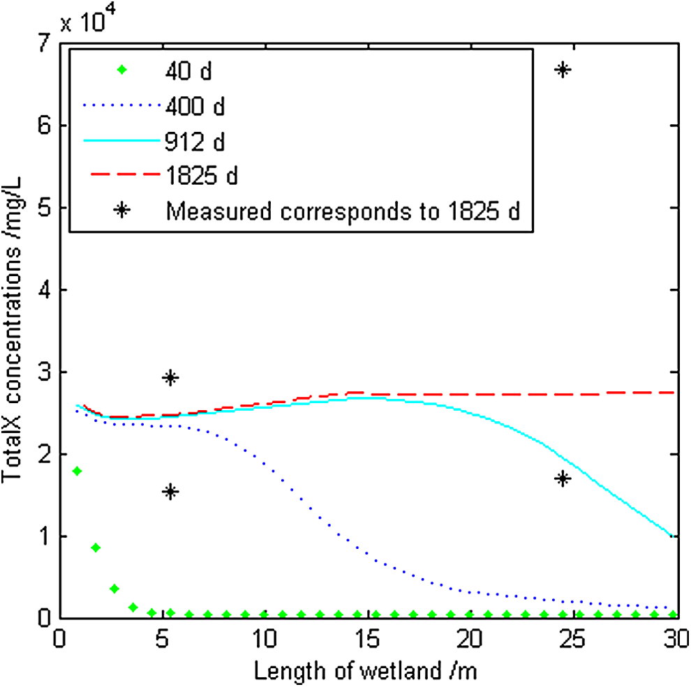
Measured results and predicted total particle concentration (Total X) profiles versus length of wetland for different operation times with the established model. Total particulate components (TotalX) = XS + XI + XH + XFB + XAMB; XS = slowly biodegradable particulate; XI = inert particulate; XH = heterotrophic bacteria; XFB = fermenting bacteria; XAMB = acetotrophic methanogenic bacteria. The measured data set came from the studies of Llorens et al. (2009).

Parameter evaluation was approximated by comparing the four plots of the measured data with the predicted concentrations of 1825 d. The key parameter R was determined as 0.0043. Nevertheless, the results showed that the proposed model can simulate the clogging processes by taking total particle concentrations within the interstitial space as indicators. This method of clogging simulation was workable.

Spatial and temporal distribution of total particle concentrations for this wetland were predicted using the parameter values determined in the model calibration and the conditions shown in Table 3 (Fig. 3). Figure 3 implies the maximum total particle concentration that occurred in the last part of the wetland after 5 years of operation. This implication agrees with the tendency of the data measured, in which the outlet zone values are higher than the inlet zone values. However, with the restricted operation time of 1 year, the total particle concentrations in the front part of the wetland are greater than those in the rear part.

FIG. 3.

Spatial–temporal distribution of the total particulate component concentrations. TotalX = XS + XI + XH + XFB + XAMB; XS = slowly biodegradable particulate; XI = inert particulate; XH = heterotrophic bacteria; XFB = fermenting bacteria; XAMB = acetotrophic methanogenic bacteria.

Profiles of particulate component concentrations versus time in the first computational unit are shown in Fig. 4 to clarify the clogging mechanism. The total concentration of particulate components in the first computational unit increased rapidly in the first 120 days and then increased gradually to a maximum value of about 25,000 mg/L. According to the former assumption, clogging occurs when the particulate matter concentration reached 32 kg (bacterial COD)/m³. Calculation using Equation (4) showed that the porosity of the first computational unit along the length of the wetland dropped to 0.4 × (1−25,000/32,000) = 0.088. This phenomenon weakened the conductivity capacity and increased probability of wetland clogging seriously.

FIG. 4.

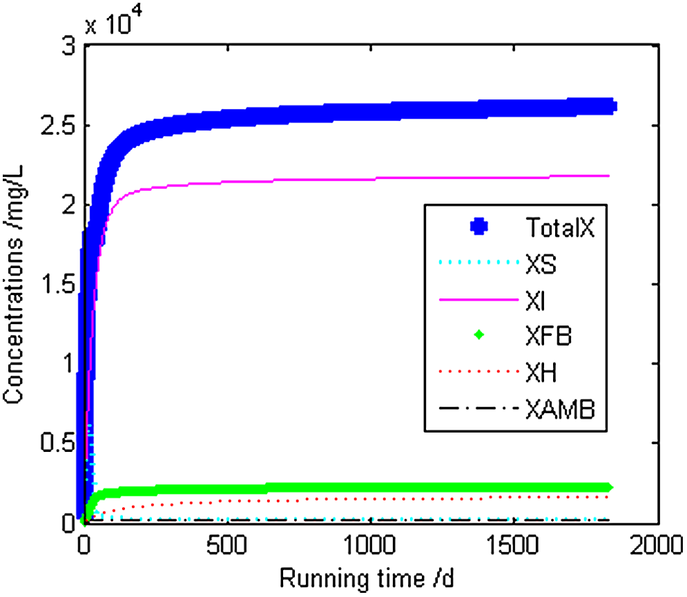
Profiles of total particulate component concentrations vs. time in the first computational unit. TotalX = XS + XI + XH + XFB + XAMB; XS = slowly biodegradable particulate; XI = inert particulate; XFB = fermenting bacteria; XH = heterotrophic bacteria; XAMB = acetotrophic methanogenic bacteria.

Figure 4 also shows that clogging at the front part of the wetland contributed to about 80% by the accumulation of X_I (nonbiodegradable particulate) and 20% by the active microorganism (X_FB, X_H, and X_AMB). Studies reported that 73% of wetland clogging was caused by organic deposits that originated from applied wastewater and above-ground plant litters (Nguyen, 2000). Moreover, the simulation of the model basically corresponded with the results reported.

Predicted total particle concentration (Total X) profiles versus time for the last substrate unit are shown in Fig. 5. The total concentration of particulate component in the last computational unit increased slowly in the first 750 days and increased quickly to a maximum value of about 27,500 mg/L. As calculated with Equation (4), the porosity of the last computational unit dropped to 0.4 × (1 − 27,500/32,000) = 0.056. This finding indicated that conductivity capacity and the probability of clogging in the rear part of the wetlands were more severe than those at the front part. Figure 5 also indicates that clogging occurred in the rear part of the wetland, which mostly results from nonbiodegradable particulates (X_I).

FIG. 5.

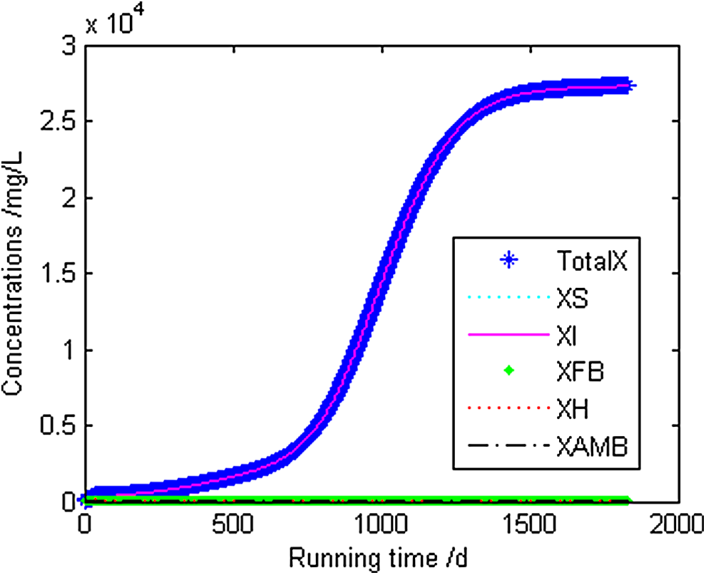
Profiles of total particulate component concentrations vs. time in the last computational unit. TotalX = XS + XI + XFB + XH + XAMB; XS = slowly biodegradable particulate; XI = inert particulate; XFB = fermenting bacteria; XH = heterotrophic bacteria; XAMB = acetotrophic methanogenic bacteria.

Conclusions

A mathematical model was developed by coupling one-dimensional mass transfer model with CWM1 model, which exhibits multicomponent biochemical reactions. Complex relations among porosity, hydraulic conductivity, and retention capability of particles were dodged dexterously in the new model by using total particle concentration within interstitial space as indicator of clogging. The particulate component release ratio was introduced as the key parameter for controlling the transmission of particles between computational units. Using the particulate component release ratio and porosity as constants could reduce the computational time and simplify the estimation for clogging. The proposed model is a simple method for prediction of HSSFCW clogging.

Mathematical stimulations showed that the proposed model could interpret the clogging mechanism of this HSSFCW. On one hand, the maximum concentration of particulate matter could occur in the front part of the wetland when running time was relatively short, such as 1 or 2 years. On the other hand, the maximum concentration of particulate matter could occur in the rear part of the wetland when running time was relatively long, such as longer than 5 years. Wetland clogging was mainly caused by the influent nonbiodegradable particulates and bacterial decay products within the interstitial space of the substrate.

Footnotes

Acknowledgment

This work was supported by the Shaanxi Province Science and Technology Development Program (Grant No. 2014K15-03-02).

Author Disclosure Statement

No competing financial interests exist.

References

Blazejewski

, and Murat-Blazejewska

(1997). Soil clogging phenomena in constructed wetlands with subsurface flow. Water Sci. Technol., 35, 183.

Boller

M.A.

, and Kavanaugh

M.C.

(1995). Particle characteristics and headloss increase in granular media filtration. Water Res. 29, 1139.

Cooper

P.F.

, Job

J.D.

, Green

, and Shutes

R.B.E.

(1996). Reed Beds and Constructed Wetlands for Wastewater Treatment. Swindon, United Kingdom: WRc Publications, p.184.

Giraldi

, Vitturi

M.D.M.

, and Iannelli

(2010). FITOVERT: A dynamic numerical model of subsurface vertical flow constructed wetlands. Environ. Model. Softw., 25, 633.

Griffin

, Wilson

, and Cooper

(2008). Changes in the use, operation and design of sub-surface flow constructed wetlands in a major UK water utility. Presented at the Proceedings of the 11th International Conference on Wetland Systems for Water Pollution Control, November, Vikram University and IWA, Indore, India, p. 419.

Hua

G.F.

, Zhu

, and Zhang

Y.H.

(2010). A conceptual approach based on suspended solids to estimate clogging time in constructed wetlands. J. Environ. Sci. Heal. Part A., 45, 1519.

Hyánková

, Kri_ska-Dunajský

, Rozko_sný

, and Sálek

(2006). The knowledge based on the research of the filtration properties of the filter media and on the determination of clogging causes. Presented at the Proceedings of the 10th International Conference on Wetland Systems for Water Pollution Control, September, Lisbon, Portugal, p. 1331.

Kadlec

R.H.

, and Wallace

S.D.

(2009). Treatment Wetlands, second ed. Boca Raton, FL: CRC Press, p. 744.

Knowles

P.R.

, and Davies

P.A.

(2011). A finite element approach to modelling the hydrological regime in horizontal subsurface flow constructed wetlands for wastewater treatment. In Vymazal

, Ed., Water and Nutrient Management in Natural and Constructed Wetlands. Dordrecht, Netherlands: Springer, p. 85.

10.

Langergraber

, Haberl

, Laber

, et al. (2004). Evaluation of substrate clogging processes in vertical flow constructed wetlands. Water Sci. Technol., 48, 25.

11.

Langergraber

, and Šimůnek

(2006). The Multi-Component Reactive Transport Module CW2D for Constructed Wetlands for the HYDRUS Software Package, Manual (Version 1.0). University of Natural Resources and Applied Life Sciences, Vienna, Austria, p. 13.

12.

Langergraber

, Rousseau

D.P.L.

, Garcia

, and Mena

(2009). CWM1: A general model to describe biokinetic processes in subsurface flow constructed wetlands. Water Sci. Technol., 59, 1687.

13.

Llorens

, Puigagut

, and Garcia

(2009). Distribution and biodegradability of sludge accumulated in a full-scale horizontal subsurface-flow constructed wetland. Desalination Water Treat. 4, 54.

14.

Nguyen

(2000). Organic matter composition, microbial biomass and microbial activity in gravel- bed constructed wetlands treating farm dairy wastewaters. Ecol. Eng., 16, 199.

15.

Nivala

, Knowles

, Dotro

, Garcıa

, and Wallace

(2012). Clogging in subsurface-flow treatment wetlands: Measurement, modeling and management. Water Res. 46, 1625.

16.

Pedescoll

, Uggetti

, Llorens

, Granés

, García

, and García

(2009). Practical method based on hydraulic conductivity used to assess clogging in subsurface flow constructed wetlands. Ecol. Eng., 35, 1216.

17.

Platzer

, and Mauch

(1997). Soil clogging in vertical flow reed beds: Mechanisms, parameters, consequences and solutions. Water Sci. Technol., 35, 175.

18.

USEPA. (1993). Subsurface Flower Constructed Wetlands for Wastewater Treatment. Washington, DC: USEPA 832-R-93–008. p. 4–1.

19.

Winter

K.J.

, and Goetz

(2003). The impact of sewage composition on the soil clogging phenomena of vertical flow constructed wetlands. Water Sci. Technol., 48, 9.

20.

Zhao

Y.Q.

, Sun

, and Allen

S.J.

(2004). Anti-sized reed bed system for animal wastewater treatment: A comparative study. Water Res. 38, 2907.