A Wind-Driven Gas Exchange Rate Model

Introduction

The dissolved oxygen is a major factor influencing the water quality of a water body. The gas exchange rate determines the speed that the dissolved oxygen transfers from the atmosphere to the water. In the wind-driven gas exchange systems turbulence is generated at the atmosphere–water interface, which is the force driving the surface renewal movement of the water parcels and determines the gas exchange rate (Komori et al., 1993; McGillis et al., 2004; Zappa et al., 2007; Duan et al., 2009a; Vachon et al., 2010). Empirical relationships have been established for the wind-driven gas exchange rate based on experiments in wind tunnels (Broecker et al., 1978; Jahne et al., 1979; Iwano et al., 2013) and experiments in oceans (Liss and Merlivat, 1986; Wanninkhof, 1992; Wanninkhof and McGillis, 1999; McNeil and D'Asaro, 2007). Another gas exchange rate formula was established using the revised global ocean ¹⁴C inventories (Wanninkhof and Feely, 2004). However, when these empirical formulae are compared big disagreements can be found although each of them adequately describes their data sets of gas exchange rate (Ro et al., 2007). The empirical formulae are normally limited in their applicability due to the specific experimental conditions under which they were developed. Further, the empirical formulae cannot explain the mechanisms of wind-driven gas exchange rate. A more generally applicable mechanistic model is needed. This study is to develop a mechanistic wind-driven gas exchange rate model by innovatively using the surface renewal mechanism and the two-film transfer mechanism together for the general application ranges. In the wind-driven gas exchange systems the gas goes through a viscous layer at the atmosphere–water interface, where the two-film transfer mechanism is predominant and then a turbulent layer where the surface renewal mechanism is predominant.

Materials and Methods

In the wind-driven gas exchange systems the shear force at the atmosphere–water interface exerted by winds establishes a turbulent boundary layer in the water phase and a second one in the atmosphere phase. The turbulent boundary layer in the water phase is much more significant as the stagnant liquid film in the water phase is predominant in the gas exchange process comparing with the stagnant gas film in the atmosphere phase. The turbulent boundary layer includes a viscous layer at the atmosphere–water interface and a turbulent layer in the space away from the atmosphere–water interface. In the wind-driven gas exchange systems the total gas exchange rate is considered in this study as the serial resistance result of that in the viscous layer and that in the turbulent layer: \documentclass{aastex}\usepackage{amsbsy}\usepackage{amsfonts}\usepackage{amssymb}\usepackage{bm}\usepackage{mathrsfs}\usepackage{pifont}\usepackage{stmaryrd}\usepackage{textcomp}\usepackage{portland, xspace}\usepackage{amsmath, amsxtra}\usepackage{upgreek}\pagestyle{empty}\DeclareMathSizes{10}{9}{7}{6}\begin{document} \begin{align*} { K_L } = { \frac { { K_ { Lv } } { K_ { L \tau } } } { { K_ { L \tau } } + { K_ { Lv } } } } , \tag { 1 } \end{align*} \end{document}

where K_L = total gas exchange rate, m/s; K_Lτ = gas exchange rate in the turbulent layer, m/s; K_Lv = gas exchange rate in the viscous layer, m/s.

The viscous layer is a stagnant liquid film where the viscosity resistance is predominant and the molecular diffusion is the major force driving the gas exchange rate. When the surface roughness is ignorable the gas exchange rate can be determined per the Two-film Theory (Richardson, 1989) and the viscous layer thickness (White, 2006) as \documentclass{aastex}\usepackage{amsbsy}\usepackage{amsfonts}\usepackage{amssymb}\usepackage{bm}\usepackage{mathrsfs}\usepackage{pifont}\usepackage{stmaryrd}\usepackage{textcomp}\usepackage{portland, xspace}\usepackage{amsmath, amsxtra}\usepackage{upgreek}\pagestyle{empty}\DeclareMathSizes{10}{9}{7}{6}\begin{document} \begin{align*} { K_ { Lv } } = \frac { D } { { { \delta _ { ve } } } } = { \frac { D { u_* } } { \Gamma \nu } } , \tag { 2 } \end{align*} \end{document}

where D = coefficient of diffusion, m²/s; δ_ve = effective thickness of viscous layer that equals to viscous layer thickness minus surface roughness, m; ν = kinematic viscosity, m²/s; u_* = shear velocity, m/s; Γ = the effective coefficient of viscous layer thickness. The viscous layer refers to the combination of the linear layer and the buffer layer in the turbulent boundary layer. For the water–bed interface, the effective coefficient of viscous layer thickness has a constant value of 35 for an atmospheric pressure of 1 atmosphere and an atmospheric temperature of 20°C (White, 2006); for the atmosphere–water interface, O'Connor (1983) employed a variable value of the effective coefficient of viscous layer thickness. In wind-driven system a surface roughness is established by friction at the atmosphere–water interface. The surface roughness pierces into the viscous layer and reduces the resistance of the viscous layer to the gas exchange. Thus, as shown in Equation (3) in Table 1, the effective viscous layer thickness \documentclass{aastex}\usepackage{amsbsy}\usepackage{amsfonts}\usepackage{amssymb}\usepackage{bm}\usepackage{mathrsfs}\usepackage{pifont}\usepackage{stmaryrd}\usepackage{textcomp}\usepackage{portland, xspace}\usepackage{amsmath, amsxtra}\usepackage{upgreek}\pagestyle{empty}\DeclareMathSizes{10}{9}{7}{6}\begin{document} $${ \delta _{ve}}$$ \end{document} equals to the viscous layer thickness \documentclass{aastex}\usepackage{amsbsy}\usepackage{amsfonts}\usepackage{amssymb}\usepackage{bm}\usepackage{mathrsfs}\usepackage{pifont}\usepackage{stmaryrd}\usepackage{textcomp}\usepackage{portland, xspace}\usepackage{amsmath, amsxtra}\usepackage{upgreek}\pagestyle{empty}\DeclareMathSizes{10}{9}{7}{6}\begin{document} $${ \delta _v}$$ \end{document} minus the surface roughness z, which is the actual distance where the transferring gas bears the viscosity resistance. The surface roughness reduces the distance of viscosity resistance. As the roughness thickness formula has three segments (Duan et al., 2009a), the effective viscous layer thickness has three formula segments as Equation (3) in Table 1 shows. In the first segment, the shear velocity is small and the atmosphere–water interface is aerodynamically smooth. The roughness coefficient at aerodynamically smooth interface, \documentclass{aastex}\usepackage{amsbsy}\usepackage{amsfonts}\usepackage{amssymb}\usepackage{bm}\usepackage{mathrsfs}\usepackage{pifont}\usepackage{stmaryrd}\usepackage{textcomp}\usepackage{portland, xspace}\usepackage{amsmath, amsxtra}\usepackage{upgreek}\pagestyle{empty}\DeclareMathSizes{10}{9}{7}{6}\begin{document} $${ \lambda _l}$$ \end{document} , is the reciprocal of a Reynolds number. The surface roughness is reversely proportional to the shear velocity. In the second segment, the atmosphere–water interface is aerodynamically rough. The shear velocity increases with the increase of the wind speed. The roughness coefficient at aerodynamically rough interface, \documentclass{aastex}\usepackage{amsbsy}\usepackage{amsfonts}\usepackage{amssymb}\usepackage{bm}\usepackage{mathrsfs}\usepackage{pifont}\usepackage{stmaryrd}\usepackage{textcomp}\usepackage{portland, xspace}\usepackage{amsmath, amsxtra}\usepackage{upgreek}\pagestyle{empty}\DeclareMathSizes{10}{9}{7}{6}\begin{document} $$\alpha$$ \end{document} , is the reciprocal of square of Froude number. The constant value 4 is used for \documentclass{aastex}\usepackage{amsbsy}\usepackage{amsfonts}\usepackage{amssymb}\usepackage{bm}\usepackage{mathrsfs}\usepackage{pifont}\usepackage{stmaryrd}\usepackage{textcomp}\usepackage{portland, xspace}\usepackage{amsmath, amsxtra}\usepackage{upgreek}\pagestyle{empty}\DeclareMathSizes{10}{9}{7}{6}\begin{document} $$\alpha$$ \end{document} and 6 is used for \documentclass{aastex}\usepackage{amsbsy}\usepackage{amsfonts}\usepackage{amssymb}\usepackage{bm}\usepackage{mathrsfs}\usepackage{pifont}\usepackage{stmaryrd}\usepackage{textcomp}\usepackage{portland, xspace}\usepackage{amsmath, amsxtra}\usepackage{upgreek}\pagestyle{empty}\DeclareMathSizes{10}{9}{7}{6}\begin{document} $${ \lambda _l}$$ \end{document} (O'Connor, 1983). The surface roughness is proportional to the square of the shear velocity. The surface roughness quickly invades the viscous layer thickness. In the third segment when the shear velocity caused by the wind speed is large enough, the surface roughness completely pierces through the whole viscous layer and thus the effective viscous layer thickness \documentclass{aastex}\usepackage{amsbsy}\usepackage{amsfonts}\usepackage{amssymb}\usepackage{bm}\usepackage{mathrsfs}\usepackage{pifont}\usepackage{stmaryrd}\usepackage{textcomp}\usepackage{portland, xspace}\usepackage{amsmath, amsxtra}\usepackage{upgreek}\pagestyle{empty}\DeclareMathSizes{10}{9}{7}{6}\begin{document} $${ \delta _{ve}}$$ \end{document} becomes zero (O'Connor, 1983). The shear velocity range for each segment can be obtained by the formulae in the column “Ranges of shear velocity” in Table 1.

Substitution of Equation (3) in Table 1 into Equation (2) yields the gas exchange rate controlled by molecular diffusion, K_Lv, as Equation (4) in Table 2.

The turbulent diffusion is the predominant force driving the gas exchange rate in the turbulent layer. The surface renewal rate is determined by the shear velocity and the turbulent boundary layer thickness as (Duan et al., 2009a) \documentclass{aastex}\usepackage{amsbsy}\usepackage{amsfonts}\usepackage{amssymb}\usepackage{bm}\usepackage{mathrsfs}\usepackage{pifont}\usepackage{stmaryrd}\usepackage{textcomp}\usepackage{portland, xspace}\usepackage{amsmath, amsxtra}\usepackage{upgreek}\pagestyle{empty}\DeclareMathSizes{10}{9}{7}{6}\begin{document} \begin{align*} r = { \frac { { u_* } } { 0.09 \delta } } , \tag { 3 } \end{align*} \end{document}

where r = surface renewal rate, s⁻¹; δ = turbulent boundary layer thickness, m. The ratio of the viscous layer thickness in the turbulent boundary layer and the turbulent boundary layer thickness is (Richardson, 1989) \documentclass{aastex}\usepackage{amsbsy}\usepackage{amsfonts}\usepackage{amssymb}\usepackage{bm}\usepackage{mathrsfs}\usepackage{pifont}\usepackage{stmaryrd}\usepackage{textcomp}\usepackage{portland, xspace}\usepackage{amsmath, amsxtra}\usepackage{upgreek}\pagestyle{empty}\DeclareMathSizes{10}{9}{7}{6}\begin{document} \begin{align*} \frac { { { \delta _v } } } { \delta } = 0.027 , \tag { 4 } \end{align*} \end{document}

where \documentclass{aastex}\usepackage{amsbsy}\usepackage{amsfonts}\usepackage{amssymb}\usepackage{bm}\usepackage{mathrsfs}\usepackage{pifont}\usepackage{stmaryrd}\usepackage{textcomp}\usepackage{portland, xspace}\usepackage{amsmath, amsxtra}\usepackage{upgreek}\pagestyle{empty}\DeclareMathSizes{10}{9}{7}{6}\begin{document} $${ \delta _v}$$ \end{document}  = the viscous layer thickness, m. Substitution of Equations (2) and (6) into Equation (5) yields since the surface roughness, z, is ignored ( \documentclass{aastex}\usepackage{amsbsy}\usepackage{amsfonts}\usepackage{amssymb}\usepackage{bm}\usepackage{mathrsfs}\usepackage{pifont}\usepackage{stmaryrd}\usepackage{textcomp}\usepackage{portland, xspace}\usepackage{amsmath, amsxtra}\usepackage{upgreek}\pagestyle{empty}\DeclareMathSizes{10}{9}{7}{6}\begin{document} $${ \delta _{ve}}$$ \end{document}  =  \documentclass{aastex}\usepackage{amsbsy}\usepackage{amsfonts}\usepackage{amssymb}\usepackage{bm}\usepackage{mathrsfs}\usepackage{pifont}\usepackage{stmaryrd}\usepackage{textcomp}\usepackage{portland, xspace}\usepackage{amsmath, amsxtra}\usepackage{upgreek}\pagestyle{empty}\DeclareMathSizes{10}{9}{7}{6}\begin{document} $${ \delta _v}$$ \end{document} ): \documentclass{aastex}\usepackage{amsbsy}\usepackage{amsfonts}\usepackage{amssymb}\usepackage{bm}\usepackage{mathrsfs}\usepackage{pifont}\usepackage{stmaryrd}\usepackage{textcomp}\usepackage{portland, xspace}\usepackage{amsmath, amsxtra}\usepackage{upgreek}\pagestyle{empty}\DeclareMathSizes{10}{9}{7}{6}\begin{document} \begin{align*} r = { \frac { 0.3 { u_* } ^2 } { \Gamma \nu } } . \tag { 5 } \end{align*} \end{document}

The surface renewal theory has been used for modeling gas exchange rate before (Duan et al., 2009a, 2009b). According to the surface renewal theory Equation (7) can yield as \documentclass{aastex}\usepackage{amsbsy}\usepackage{amsfonts}\usepackage{amssymb}\usepackage{bm}\usepackage{mathrsfs}\usepackage{pifont}\usepackage{stmaryrd}\usepackage{textcomp}\usepackage{portland, xspace}\usepackage{amsmath, amsxtra}\usepackage{upgreek}\pagestyle{empty}\DeclareMathSizes{10}{9}{7}{6}\begin{document} \begin{align*} { K_ { L \tau } } = \sqrt { Dr } = \sqrt { { \frac { 0.3D { u_* } ^2 } { \Gamma \nu } } } . \tag { 6 } \end{align*} \end{document}

Substitution of Equations (4) and (8) into Equation (1) yields Equation (9) in Table 3, which is the model and formula of the wind-driven gas exchange rate in terms of shear velocity developed in this study.

At the atmosphere–water interface, the shear velocity is determined by the skin-friction coefficient at atmosphere–water interface and the free flow velocity if only the streamflow is the driving force (White, 2006): \documentclass{aastex}\usepackage{amsbsy}\usepackage{amsfonts}\usepackage{amssymb}\usepackage{bm}\usepackage{mathrsfs}\usepackage{pifont}\usepackage{stmaryrd}\usepackage{textcomp}\usepackage{portland, xspace}\usepackage{amsmath, amsxtra}\usepackage{upgreek}\pagestyle{empty}\DeclareMathSizes{10}{9}{7}{6}\begin{document} \begin{align*} { u_* } = \sqrt { \frac { { { C_f } } } { 2 } } U , \tag { 7 } \end{align*} \end{document}

where u_* = shear velocity at atmosphere–water interface, m/s; U = flow velocity, m/s; and C_f = skin-friction coefficient at atmosphere–water interface. The relationship between the shear velocity in water phase and that in atmosphere phase is (O'Connor, 1983) \documentclass{aastex}\usepackage{amsbsy}\usepackage{amsfonts}\usepackage{amssymb}\usepackage{bm}\usepackage{mathrsfs}\usepackage{pifont}\usepackage{stmaryrd}\usepackage{textcomp}\usepackage{portland, xspace}\usepackage{amsmath, amsxtra}\usepackage{upgreek}\pagestyle{empty}\DeclareMathSizes{10}{9}{7}{6}\begin{document} \begin{align*} { u_ { *w } } = \sqrt { { \frac { { \rho _a } } { { \rho _w } } } } { u_ { *a } } , \tag { 8 } \end{align*} \end{document}

where u_*a = shear velocity at the atmosphere–water interface in atmosphere phase, m/s; u_*w = shear velocity at the atmosphere–water interface in water phase, m/s; ρ_a = density of atmosphere, kg/m³; and ρ_w = density of water, kg/m³. Substitution of Equation (10) into Equation (11) yields \documentclass{aastex}\usepackage{amsbsy}\usepackage{amsfonts}\usepackage{amssymb}\usepackage{bm}\usepackage{mathrsfs}\usepackage{pifont}\usepackage{stmaryrd}\usepackage{textcomp}\usepackage{portland, xspace}\usepackage{amsmath, amsxtra}\usepackage{upgreek}\pagestyle{empty}\DeclareMathSizes{10}{9}{7}{6}\begin{document} \begin{align*} { u_* } = { u_ { *w } } = \sqrt { { \frac { { \rho _a } } { { \rho _w } } } } { u_ { *a } } = \sqrt { { \frac { { \rho _a } } { { \rho _w } } } } \sqrt { \frac { { { C_f } } } { 2 } } W , \tag { 9 } \end{align*} \end{document}

where W = wind speed at 10 m above water surface, which is the flow velocity U in Equation (10), m/s. The model of the wind-driven gas exchange rate developed in this study is described as Equations (9) and (12).

Results and Discussion

The model of the wind-driven gas exchange rate developed in this study described as Equations (9) and (12) can be rewritten as a function of wind speed as Equation (13) in Table 4. The first and third segments of Equation (13) in Table 4 have similar terms as those of Liss–Merlivat empirical formula on wind-driven gas exchange rate (Liss and Merlivat, 1986) in Equation (14) in Table 5. The second segment of Equation (14) in Table 5 can be considered as a simplified approximate term of the second segment of Equation (13) in Table 4, which is for the transition zone when the surface roughness pierces through the viscous layer. Then the turbulence in the air phase and the turbulence in the water phase touch each other, which accelerates the gas exchange rate. Equation (13) in Table 4 is the general formula, whereas Equation (14) in Table 5 is a special case obtained with specific experimental data set. The empirical coefficients in the first and third segments of Liss–Merlivat empirical formula obtained from experiments can now be explained with the first and third segments of the mechanistic formulae in Equations (9), (12), and (13) in Table 4. The second segment of Liss–Merlivat empirical formula is a transition between the first and third segments and can now be considered a simplified approximate format of the second segment of the mechanistic formulae developed in this study, which represents the influence of the surface roughness' development to the effective viscous layer thickness. C_f can be directly calculated from z by the log law. But the manner of variable C_f yields iterative calculation in Table 4. To overcome this iterative problem, constant C_f of 4.0 × 10⁻³ is employed in this study to calculate gas exchange rate under the normal wind speed (O'Connor, 1983).

OPEN IN VIEWER

Table 4.

Wind-Driven Gas Exchange Rate in Terms of Wind Speed [Eq. (13)]

The comparison of the predictions of the wind-driven gas exchange rate model developed in this study [Eq. (13) in Table 4] and the Liss–Merlivat empirical formula [Eq. (14) in Table 5; Liss and Merlivat, 1986] is shown in Fig. 1. Each of these two curves has three segments corresponding to the three segments in their formulae. Segment 1 represents that when the wind speed is small the surface roughness is reversely proportional to the shear velocity. Segment 2 represents that when the wind speed increases the surface roughness is proportional to the square of the shear velocity. Segment 2 is a complex curve represented as in the mechanistic formula developed in this study [Eq. (13) in Table 4]. Whereas as an empirical formula the Liss–Merlivat formula [Eq. (14) in Table 5] uses a straight line to roughly describe Segment 2. Segment 3 represents that when the wind speed is large enough the surface roughness completely pierces through the whole viscous layer and thus the effective viscous layer thickness \documentclass{aastex}\usepackage{amsbsy}\usepackage{amsfonts}\usepackage{amssymb}\usepackage{bm}\usepackage{mathrsfs}\usepackage{pifont}\usepackage{stmaryrd}\usepackage{textcomp}\usepackage{portland, xspace}\usepackage{amsmath, amsxtra}\usepackage{upgreek}\pagestyle{empty}\DeclareMathSizes{10}{9}{7}{6}\begin{document} $${ \delta _{ve}}$$ \end{document} becomes zero as shown in Equation (3) in Table 1.

OPEN IN VIEWER

FIG. 1.

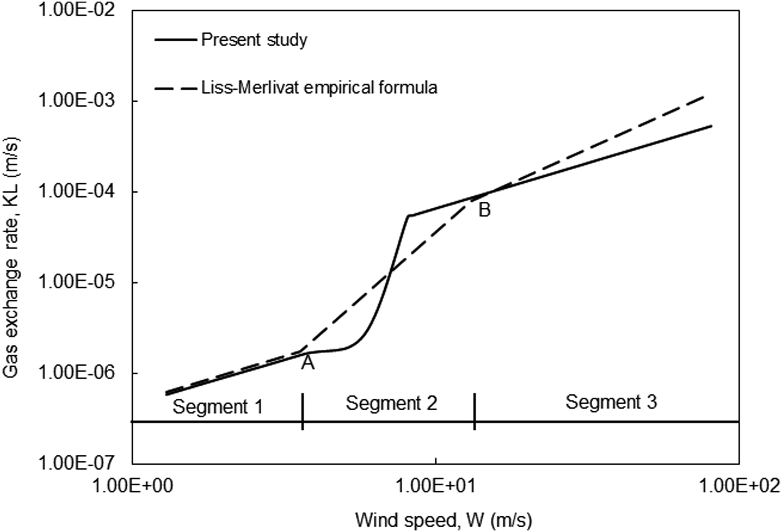
Comparison of the predictions of the wind-driven gas exchange rate model developed in this study [Eq. (13) in Table 4] and the Liss–Merlivat empirical formula [Eq. (14) in Table 5; Liss and Merlivat, 1986]. The three segments of Equation (14) in Table 5 are left to A (Segment 1), A to B (Segment 2), and B to right (Segment 3).

Experimental data sets are employed to compare with the predictions of the wind-driven gas exchange rate model developed in this study. MacIntyre et al. (1995) investigated the gas exchange rate in some lakes with different wind speeds and obtained the related experimental data set. Law and Khoo (2002) measured the gas exchange rate in a circular wind channel. Broecker et al. (1978) measured the gas exchange rate in a large wind tunnel. Jahne et al. (1979) did experiments on wind-driven gas exchange rate in a wind tunnel. As Fig. 2 shows, the predictions of the wind-driven gas exchange rate model developed in this study have reasonable agreements with the experimental data sets. The absolute values of difference magnitudes of the predictions of the wind-driven gas exchange rate model developed in this study and the experimental data range from 2.00 × 10⁻⁷ m/s to 3.55 × 10⁻⁵ m/s. The absolute values of difference percentages of the predictions of the wind-driven gas exchange rate model developed in this study and the experimental data range from 0.57% to 52.07%. The coefficient of determination in Table 6 indicated that the wind-driven gas exchange rate model developed in this study explained from 83% to 96% of the variability in the experimental data in both laboratory and field measurements. The predictions of the model developed in this study as Equations (9) and (12) agree well with the measured data.

OPEN IN VIEWER

FIG. 2.

Comparison of the predictions of the wind-driven gas exchange rate model developed in this study and the experimental data.

As Fig. 2 shows, the deviations between the experimental data and the predicted values become relatively large for the higher gas exchange rate values. The wind speed is large for those higher gas exchange rate values. When the wind speed becomes large, the wave breaking and bubble-mediated gas exchange may occur, which increases the total gas exchange rate and causes the deviations between the experimental data and the predicted values. Thus, the predictive model has a relatively better performance in the lower gas exchange rate than in the higher gas exchange rate. The applied conditions of this study are for wind speed less than about 30 m/s as shown in Fig. 1. The limitations of this study is that it will underestimate the gas exchange rate when wind is large enough and the wave breaking and bubble-mediated gas exchange may occur. As a possible improvement these facts need to be considered and included in the wind-driven gas exchange rate model in future.

Conclusions

A mechanistic model of wind-driven gas exchange rate is developed in this study based on the surface renewal mechanism and the two-film transfer mechanism. The total gas exchange rate is the serial resistance result of that in the viscous layer and that in the turbulent layer. The viscosity layer thickness minus the surface roughness is the actual distance where the transferring gas bears the viscosity resistance at the atmosphere–water interface in wind-driven system. The surface roughness reduces the distance of viscosity resistance. The predictions of the wind-driven gas exchange rate mechanistic model developed in this study have reasonable agreements with the experimental data sets from laboratory and field measurements. This mechanistic model can be applied for water bodies with wind as the predominant force driving the gas exchange rate of the low soluble gases, for example, dissolved oxygen and carbon dioxide.