Effect of Partially Submerged Vegetation Distribution Directions on Flood Flow Resistance

Abstract

The large-scale distribution of vegetation influences flood flow concentration. Natural and cultivated high plants impact the flood flow velocity field and volume distribution in a watershed. Many studies have examined flow resistance associated with plant density and stalk flexibility. Some researchers have explored the effect of vegetation distribution and suggest that the flow resistance changes with vegetation distribution. This assertion, however, was made without experimental verification. In our research, we built a hydraulic model with constant vegetation density and flexibility from beginning to end, which can simulate various distribution directions of partially submerged plant stems and reveal the flood flow resistance for different slope gradients. After more than 300 tests, we demonstrated that the change of partially submerged vegetation distribution direction leads to directional differences in flood flow resistance. We found that the flow resistance coefficient (f) increases linearly with increasing submergence depth (h), at an incremental rate α ( \documentclass{aastex}\usepackage{amsbsy}\usepackage{amsfonts}\usepackage{amssymb}\usepackage{bm}\usepackage{mathrsfs}\usepackage{pifont}\usepackage{stmaryrd}\usepackage{textcomp}\usepackage{portland, xspace}\usepackage{amsmath, amsxtra}\usepackage{upgreek}\pagestyle{empty}\DeclareMathSizes{10}{9}{7}{6}\begin{document} $${ \rm{ \alpha }} = df / dh$$ \end{document} ) that is influenced by the distribution directions of vegetation. In addition, we discovered that the relationship between the incremental rate (α) and the projection width of vegetation (K) on flow direction can be represented with a noteworthy power function: \documentclass{aastex}\usepackage{amsbsy}\usepackage{amsfonts}\usepackage{amssymb}\usepackage{bm}\usepackage{mathrsfs}\usepackage{pifont}\usepackage{stmaryrd}\usepackage{textcomp}\usepackage{portland, xspace}\usepackage{amsmath, amsxtra}\usepackage{upgreek}\pagestyle{empty}\DeclareMathSizes{10}{9}{7}{6}\begin{document} $$df / dh = 0.686{K^{0.304}}$$ \end{document} .

Introduction

Vegetation plays a major role in watersheds and river networks by affecting hydrological processes and influencing the flood flow velocity field and volume distribution under a variety of conditions, including different slopes and shallows.

Flood flow resistance varies due to a range of factors, including plant density, flexibility, cross-sectional area, quantity of branches, and leaf cover. In recent years, numerous researchers have focused on the influence of vegetation density on flow resistance (Nepf, 1999; Cheng, 2011; Neary et al., 2012). For example, researchers simulated flow resistance in an open channel resulting from vegetation of different densities and diameters (Cheng and Nguyen, 2011; Liu et al., 2018). It is well known that the flexibility and quantities of branches and leaves, submerged flexible herbaceous vegetation, and nonsubmerged woody vegetation also have certain effects on flow resistance (Järvelä, 2004, 2005). Moreover, the influence of the bending rigidity of submerged vegetation on flow resistance should not be neglected (Guo et al., 2011; Wu and Yang, 2014; Liu et al., 2018). Using round bars to simulate vegetation, researchers have studied the water flow resistance of plants under submerged and nonsubmerged conditions, and they found that their resistance is related to water depth, plant density, and other factors (Stone and Shen, 2002). Experts and scientists have studied the effects of nonsubmerged vegetation on water structure and kinetic energy characteristics using pineapple branches as experimental materials (Yagci et al., 2010). Based on experiments utilizing water discharge in a flume, a formula for calculating the plant resistance coefficient was proposed from force analysis and regression of experimental data (Wu et al., 1999). Based on a physical model, and considering the influence of different vegetation distribution patterns, Luhar and Nepf (2013) concluded that the total hydraulic resistance generated by vegetation primarily depends on the blocking factor, that is, the proportion of the vegetation blocking a channel section.

There have been some studies focusing on the influence of vegetation distribution on flow resistance. Research has shown that the distribution of vegetation in the lower depths of the test section was better than that in the middle and upper regions, and it has been demonstrated that the vegetation distribution pattern has an important influence on the hydraulic characteristics of the slope (Ding and Li, 2016). Researchers have found that an irregular distribution of vegetation significantly slows flow velocity (Zhang et al., 2012). Stephan and Gutknecht (2002) showed that the change of water flow velocity in the presence of vegetation in the slope flow depends primarily on the type, density, and configuration pattern of the vegetation. Flood flow resistance is influenced significantly by the distribution of the vegetation; there is a strong relationship between vegetation distribution density and Manning resistance. The greater the vegetation distribution density in the river channel, the greater the Manning resistance and the more obvious the effect on water flow resistance (Laounia et al., 2005). Through experiments, we now understand how vegetation impacts flow and transport and how flow feedbacks influence vegetation spatial structure. When the vegetation reaches a certain density, the turbulent stress cannot penetrate into the bed, and the vegetation can then promote sediment retention and stabilize the bed. If the vegetation density is too low, the flow and pressure near the bed will increase, the resuspension of sediment will increase, and the stability of the bed will decrease (Luhar et al., 2008). Researchers believe that vegetation distribution impacts the effects of flood flow resistance. By studying staggered and nonstaggered vegetation configurations (rectangular and triangular), it has been concluded that flow pattern has little to do with vegetation configuration, and the decrease in vegetation density will lead to a decrease in flow resistance (Chen et al., 2015). Vegetation friction may be related to some other factors, such as the arrangement of the vegetation; however, this assertion has not been investigated further (Tang et al., 2014). At present, an open channel flow with a single flow direction has been utilized as the main experimental method for flow resistance in partially submerged vegetation effect simulation. These kinds of studies focus on slope gradient, vegetation type and density, and resistance associated with rainfall (Liu et al., 2010; Guo et al., 2011; Okamoto et al., 2012; Arguelles et al., 2013; Wang et al., 2015; Duan et al., 2016; Zhang et al., 2018), without considering the characteristics of flow passing through partially submerged vegetation, in conditions such as wide flat shallow areas with low velocity, or multiple flow directions. As a result, current research is yet to address the flood flow resistance changes for different flow directions with various vegetation distributions.

The influence of vegetation distribution directions on flood flow resistance is still unknown, as are the influences of other factors including surface gradient and submergence, which require further analysis. It is inappropriate to use water boundary material and particle size as indices to describe flow resistance, since neither the spatial heterogeneity of the surface material nor the relevant resistance change are accounted for (Cooper et al., 2006). Therefore, this study simulates the influence of the vegetation distribution trend on water flow resistance as well as the influence of surface slope, submergence water depth, and other factors on flow resistance by controlling density, rod diameter, roughness, and other characteristics, as well as adjusting the slope and submergence depth for various distribution trends using hydraulics experiments. This research is necessary to accurately simulate the flood flow velocity field and volume distribution for vegetation-covered slopes, and it has practical value in wetland vegetation flood storage and drainage, farm irrigation, and other areas.

The flow resistance parameters used to represent the combined flow resistance effects include the Manning roughness coefficient (n), the Chezy factor (C), and the Darcy-Weisbach resistance coefficient (f). Currently, opinions differ as to the pros and cons of these three coefficients in flow resistance representation. It is feasible to use the f∼Re relationship to predict water resistance through multiple runoff tests on the grassland and shrubs of the semiarid mountain areas of Arizona. Since the Manning coefficient (n) is more suitable for turbulent flow regimes, the flow regime of surface slopes has not yet been defined. In this case, it is inaccurate to use the Manning coefficient (n) to express flow resistance. Since f can be applied to various flow regimes, it is more appropriate to use f to represent flow resistance (Abrahams et al., 1994). By analyzing the differences between momentum resistance and energy resistance, point resistance, the resistance coefficient of section resistance, and composite channel resistance, it has been shown that the Manning coefficient (n) and the Darcy-Weisbach resistance coefficient (f) are interchangeable and theoretically equivalent. However, in practical terms, for fully developed turbulence, the Manning coefficient (n) is often considered to correspond to a rough surface that approximates a constant (Yen, 2002). The Manning roughness coefficient was tested under various flow conditions and with different vegetation parameters (Noarayanan et al., 2012), and it was regarded as a proper tool for calculating and describing the resistance for shallow sheet flow. Combining the Darcy-Weisbach resistance formula of pipe flow and the Manning formula of open channel flow to create a Manning roughness coefficient based on flow and media characteristics, relevant experimental results demonstrate that in fully turbulent flow the Manning roughness coefficient is a constant value, which is independent of flow characteristics (Sedghi-Asl and Rahimi, 2011). Only the Darcy-Weisbach resistance coefficient (f) can be applied to both laminar and turbulent flow (Cristo et al., 2012). Overland flow through vegetation is mainly cross-regime flow between laminar and turbulent flow, which is difficult to compute using the Manning formula (Kadlec, 1990). Experiments have shown that the surface distribution of flow depth and rainfall intensity influences the surface resistance distribution represented by the Manning roughness coefficient. Currently, there is considerable disagreement as to the pros and cons of the three flow resistance representations (Fraga et al., 2013). However, research indicates that the Darcy-Weisbach resistance coefficient (f) is suitable for laminar and turbulent flow, and that the Manning roughness coefficient (n) and Chezy factor (C) apply only to turbulence. In an attempt to study the flow resistance change regularity in different directional distributions of partially submerged vegetation, our research considered the Darcy-Weisbach resistance factor (f) to be the best choice, due to its applicability in different flow regimes.

Materials and Methods

Our experiment was conducted in a flume (Fig. 1), which was 12 m in length and 0.4 m in width, and it had a flank that was 0.6 m high. The open channel sink was customized at Zhejiang University in China. The pump and electromagnetic flow meter model was LDG-MIK-DN100, and the flow range was 0–1,000 m³/h. The entrance of the flume was a level water tank. The flume body was divided into three parts: an equalizing section, a middle test section, and an end gate section. Along the test section, manometry tubes were installed for observation of the hydraulic head. Containing a self-circulating water supply system and a gradient-adjusting wheel, the flume was also fitted with an electromagnetic flowmeter, a flow control valve, and a resin board (0.4 × 3.0 m) at the flume bottom. The board had holes spaced 60 mm apart both laterally and lengthwise, with an aperture of 3 mm. Plastic rods were inserted into the holes to simulate surface vegetation. Different angles of flow direction and vegetation distribution direction were simulated for various vegetation densities and flume widths by locating the rods on the board in a variety of patterns (Fig. 2). We used four vegetation simulation angles—15°, 30°, 45°, and 90°—in our experiments.

FIG. 1.

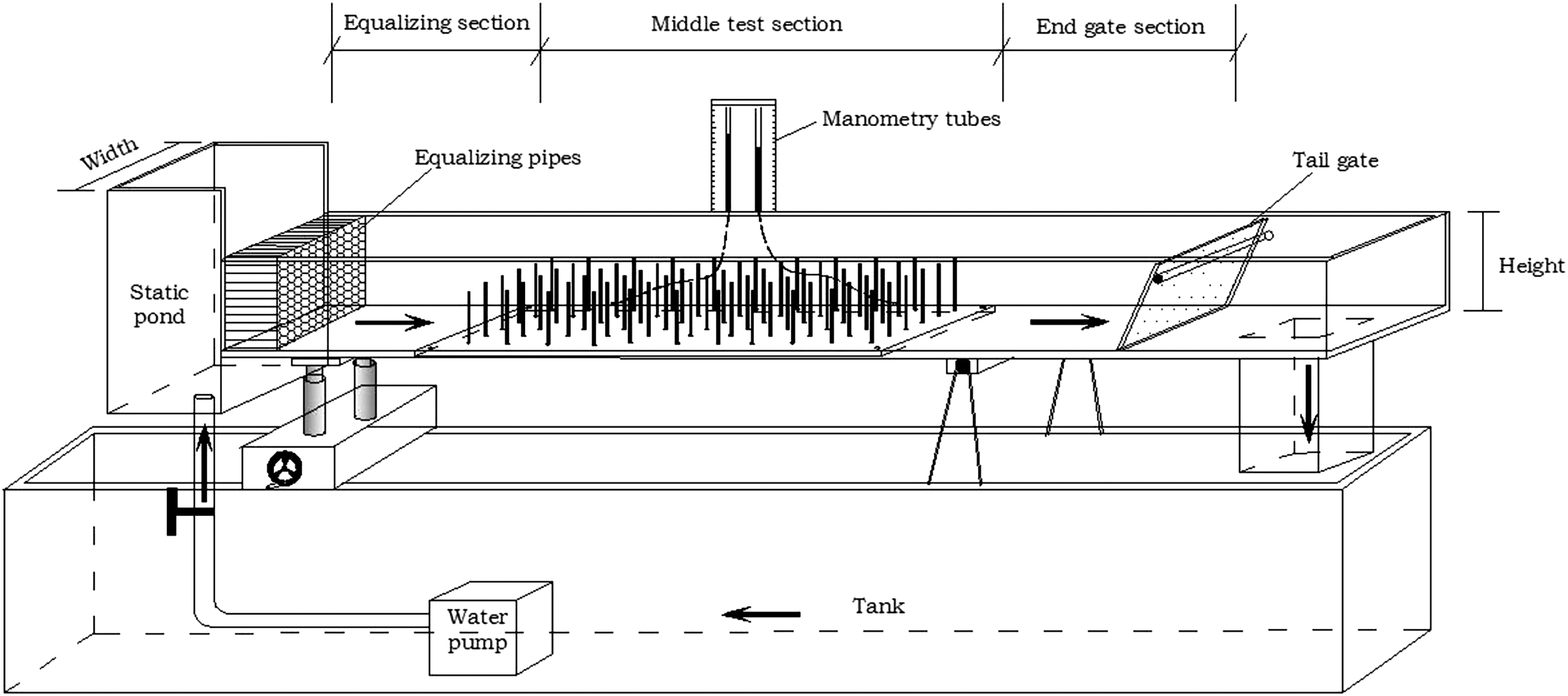
Diagram of the experimental flume, including the tank, water pump, static pond, equalizing pipes, tail gate, and manometry tubes. The flume is divided into three sections: the equalizing section, the middle test section, and the end gate section.

FIG. 2.

Schematic diagram of the vegetation distribution. \documentclass{aastex}\usepackage{amsbsy}\usepackage{amsfonts}\usepackage{amssymb}\usepackage{bm}\usepackage{mathrsfs}\usepackage{pifont}\usepackage{stmaryrd}\usepackage{textcomp}\usepackage{portland, xspace}\usepackage{amsmath, amsxtra}\usepackage{upgreek}\pagestyle{empty}\DeclareMathSizes{10}{9}{7}{6}\begin{document} $$\bar{u}$$ \end{document} is the flow direction and θ is the angle of the flow direction relative to the direction of overland strips within the a × b strip distribution.

We also adjusted the flume gradient and flow quantity to study the influence of gradient and submergence depth on flow resistance. In various tests having different distribution angles, the flume gradient was set to 0.0%, 0.5%, 1.0%, 1.5%, and 2.0%, and in every gradient we varied the flow rate 12–17 times from small to large. For example, when the rods were located at 90° in the lever flume, 16 sets of data for different flow rate conditions were observed and calculated (Table 1). The relative formulae are as follows:

Table 1.

Parameters for a Vegetation Distribution Directional Angle of 90° and a Flume Gradient of 0.0%

Experiment trails	Water level of manometry tubes, cm		Flow volume, m³/hQ	Submerged height, m		Flow velocity, m/s		Head loss, mh_f	Darcy-Weisbach friction factorf
Experiment trails	H₁	H₂	Flow volume, m³/hQ	h₁	h₂	V₁	V₂	Head loss, mh_f	Darcy-Weisbach friction factorf
1	60.75	60.52	1.46	0.01050	0.0082	0.096561	0.123645	0.001996	0.076809
2	61.24	61.02	2.51	0.01540	0.0132	0.113336	0.132225	0.001963	0.090813
3	61.50	61.28	3.15	0.01800	0.0158	0.121528	0.138449	0.001976	0.095198
4	61.88	61.69	4.05	0.02180	0.0199	0.129120	0.141448	0.001730	0.093260
5	62.35	62.12	5.28	0.02650	0.0242	0.138365	0.151515	0.002106	0.117833
6	62.54	62.32	6.04	0.02840	0.0262	0.147610	0.160005	0.002005	0.106415
7	62.78	62.51	6.77	0.03080	0.0281	0.152642	0.167309	0.002461	0.128967
8	62.98	62.75	7.51	0.03280	0.0305	0.158932	0.170917	0.002098	0.110161
9	63.25	63.00	8.38	0.03550	0.0330	0.163863	0.176277	0.002285	0.120702
10	63.49	63.20	9.17	0.03790	0.0350	0.168023	0.181944	0.002651	0.139511
11	64.09	63.79	11.56	0.04390	0.0409	0.182812	0.196222	0.002741	0.139500
12	64.92	64.63	14.84	0.05220	0.0493	0.197469	0.209085	0.002659	0.136127
13	66.12	65.72	19.89	0.06420	0.0602	0.215148	0.229444	0.003676	0.184422
14	66.91	66.49	23.53	0.07210	0.0679	0.226601	0.240618	0.003866	0.191946
15	68.42	67.93	31.06	0.08720	0.0823	0.247383	0.262111	0.004517	0.216521
16	69.85	69.32	38.72	0.10150	0.0962	0.264938	0.279534	0.004895	0.228312

\documentclass{aastex}\usepackage{amsbsy}\usepackage{amsfonts}\usepackage{amssymb}\usepackage{bm}\usepackage{mathrsfs}\usepackage{pifont}\usepackage{stmaryrd}\usepackage{textcomp}\usepackage{portland, xspace}\usepackage{amsmath, amsxtra}\usepackage{upgreek}\pagestyle{empty}\DeclareMathSizes{10}{9}{7}{6}\begin{document} \begin{align*} {h_1} = {H_1} - {Z_1}; \ {h_2} = {H_2} - {Z_2} \tag{1} \end{align*} \end{document}

\documentclass{aastex}\usepackage{amsbsy}\usepackage{amsfonts}\usepackage{amssymb}\usepackage{bm}\usepackage{mathrsfs}\usepackage{pifont}\usepackage{stmaryrd}\usepackage{textcomp}\usepackage{portland, xspace}\usepackage{amsmath, amsxtra}\usepackage{upgreek}\pagestyle{empty}\DeclareMathSizes{10}{9}{7}{6}\begin{document} \begin{align*} { h_f } = \left( { { H_1 } - { H_2 } } \right) + \left( { { \frac { V_1^2 } { 2g } } - { \frac { V_2^2 } { 2g } } } \right) \tag { 2 } \end{align*} \end{document}

\documentclass{aastex}\usepackage{amsbsy}\usepackage{amsfonts}\usepackage{amssymb}\usepackage{bm}\usepackage{mathrsfs}\usepackage{pifont}\usepackage{stmaryrd}\usepackage{textcomp}\usepackage{portland, xspace}\usepackage{amsmath, amsxtra}\usepackage{upgreek}\pagestyle{empty}\DeclareMathSizes{10}{9}{7}{6}\begin{document} \begin{align*} f = { h_f } \frac { { 4 \bar R } } { l } { \frac { 2g } { { { \bar V } ^2 } } } \tag { 3 } \end{align*} \end{document}

\documentclass{aastex}\usepackage{amsbsy}\usepackage{amsfonts}\usepackage{amssymb}\usepackage{bm}\usepackage{mathrsfs}\usepackage{pifont}\usepackage{stmaryrd}\usepackage{textcomp}\usepackage{portland, xspace}\usepackage{amsmath, amsxtra}\usepackage{upgreek}\pagestyle{empty}\DeclareMathSizes{10}{9}{7}{6}\begin{document} \begin{align*} Re = \frac { { VR } } { \nu } \tag { 4 } \end{align*} \end{document}

In these formulae, H₁ and H₂, with units of cm, are the manometry tube readings for the measured cross-sections 1 and 2, respectively; the measurement unit of the electromagnetic flowmeter is m³/s; h₁, h₂, with units of m, are the submergence depths of cross-sections 1 and 2, respectively, and are equal to the difference between the manometry tube reading and the section location height. When the flume gradient is 0.0%, the location heights of 1 and 2 (Z₁ and Z₂) are both 59.7 cm; \documentclass{aastex}\usepackage{amsbsy}\usepackage{amsfonts}\usepackage{amssymb}\usepackage{bm}\usepackage{mathrsfs}\usepackage{pifont}\usepackage{stmaryrd}\usepackage{textcomp}\usepackage{portland, xspace}\usepackage{amsmath, amsxtra}\usepackage{upgreek}\pagestyle{empty}\DeclareMathSizes{10}{9}{7}{6}\begin{document} $$\bar R$$ \end{document} , with units of m, represents the average hydraulic radius; \documentclass{aastex}\usepackage{amsbsy}\usepackage{amsfonts}\usepackage{amssymb}\usepackage{bm}\usepackage{mathrsfs}\usepackage{pifont}\usepackage{stmaryrd}\usepackage{textcomp}\usepackage{portland, xspace}\usepackage{amsmath, amsxtra}\usepackage{upgreek}\pagestyle{empty}\DeclareMathSizes{10}{9}{7}{6}\begin{document} $$\bar V$$ \end{document} , with units of m/s, is the average flow velocity; h_f is the head loss from cross-section 1 to cross-section 2 due to friction; g is the gravitational acceleration; l is the length from cross-section 1 to cross-section 2 (i.e., 1.5 m in this experiment); f is the Darcy-Weisbach resistance factor; Re is Reynolds number; and \documentclass{aastex}\usepackage{amsbsy}\usepackage{amsfonts}\usepackage{amssymb}\usepackage{bm}\usepackage{mathrsfs}\usepackage{pifont}\usepackage{stmaryrd}\usepackage{textcomp}\usepackage{portland, xspace}\usepackage{amsmath, amsxtra}\usepackage{upgreek}\pagestyle{empty}\DeclareMathSizes{10}{9}{7}{6}\begin{document} $${ \rm{ \nu }}$$ \end{document} is the kinematic viscosity coefficient.

Under controlled vegetation density and plant morphology, we conducted 321 tests for different vegetation distribution directions, slope gradients, and submergence depths, which are listed in Table 2.

Table 2.

Test Trials with Different Sets of Vegetation Distribution Directions and Slope Gradients

Vegetation distribution direction	Flume slope					Total trails
Vegetation distribution direction	0.0%	0.5%	1.0%	1.5%	2.0%	Total trails
15°	17	16	16	17	16	82
30°	17	17	17	17	17	85
45°	15	16	17	17	17	82
90°	16	14	17	13	12	72

Results

According to the experimental data from four different angles (θ) of vegetation distribution direction, we plotted a dot diagram (Fig. 3) to introduce the relation between flow depth (h) and resistance coefficient (f) with various slope gradients (i). This figure, however, shows no obvious effect of gradient on f.

FIG. 3.

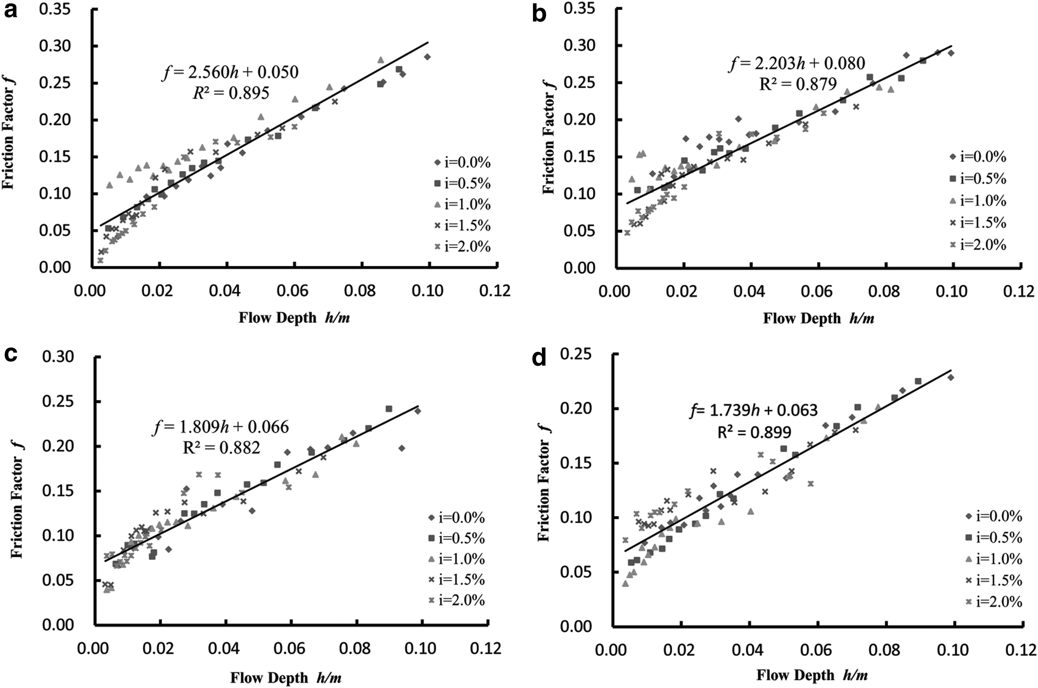
Diagram of the relationship between flow depth (h) and the Darcy-Weisbach friction factor (f). The four diagrams represent the relationship between the hydraulic changes of (h) and (f) for different slopes of four different vegetation distribution trend angles (θ). (a) θ = 15°, (b) θ = 30°, (c) θ = 45°, and (d) θ = 90°.

The centralized distribution of five gradients with the same angle (θ) of vegetation distribution direction are illustrated in Fig. 3, in which there is remarkable linear regression relationship between flow depth (h) and resistance coefficient (f), shown as follows: \documentclass{aastex}\usepackage{amsbsy}\usepackage{amsfonts}\usepackage{amssymb}\usepackage{bm}\usepackage{mathrsfs}\usepackage{pifont}\usepackage{stmaryrd}\usepackage{textcomp}\usepackage{portland, xspace}\usepackage{amsmath, amsxtra}\usepackage{upgreek}\pagestyle{empty}\DeclareMathSizes{10}{9}{7}{6}\begin{document} \begin{align*} { \rm{When}} \ \theta = 15^ \circ , \ {f_{15}} = 2.560h + 0.050 \ { \rm{ and}} \ {R^2} = 0.895 \tag{5} \end{align*} \end{document} \documentclass{aastex}\usepackage{amsbsy}\usepackage{amsfonts}\usepackage{amssymb}\usepackage{bm}\usepackage{mathrsfs}\usepackage{pifont}\usepackage{stmaryrd}\usepackage{textcomp}\usepackage{portland, xspace}\usepackage{amsmath, amsxtra}\usepackage{upgreek}\pagestyle{empty}\DeclareMathSizes{10}{9}{7}{6}\begin{document} \begin{align*} { \rm{When}} \ \theta = 30^ \circ , \ {f_{30}} = 2.203h + 0.080 \ { \rm{ and}} \ {R^2} = 0.879 \tag{6} \end{align*} \end{document}

\documentclass{aastex}\usepackage{amsbsy}\usepackage{amsfonts}\usepackage{amssymb}\usepackage{bm}\usepackage{mathrsfs}\usepackage{pifont}\usepackage{stmaryrd}\usepackage{textcomp}\usepackage{portland, xspace}\usepackage{amsmath, amsxtra}\usepackage{upgreek}\pagestyle{empty}\DeclareMathSizes{10}{9}{7}{6}\begin{document} \begin{align*} { \rm{When}} \ \theta = 45^ \circ , \ {f_{45}} = 1.809h + 0.066 \ { \rm{ and}} \ {R^2} = 0.882 \tag{7} \end{align*} \end{document}

\documentclass{aastex}\usepackage{amsbsy}\usepackage{amsfonts}\usepackage{amssymb}\usepackage{bm}\usepackage{mathrsfs}\usepackage{pifont}\usepackage{stmaryrd}\usepackage{textcomp}\usepackage{portland, xspace}\usepackage{amsmath, amsxtra}\usepackage{upgreek}\pagestyle{empty}\DeclareMathSizes{10}{9}{7}{6}\begin{document} \begin{align*} { \rm{When}} \ \theta = 90^ \circ , \ {f_{90}} = 1.739h \; + \;0.063 \ { \rm{ and}} \ {R^2} = 0.899 \tag{8} \end{align*} \end{document}

The regression equations show that the resistance coefficient (f) is linearly proportional to flow depth (h) with a high correlation regardless of the vegetation distribution direction angle (θ). The fundamental form is shown as follows: \documentclass{aastex}\usepackage{amsbsy}\usepackage{amsfonts}\usepackage{amssymb}\usepackage{bm}\usepackage{mathrsfs}\usepackage{pifont}\usepackage{stmaryrd}\usepackage{textcomp}\usepackage{portland, xspace}\usepackage{amsmath, amsxtra}\usepackage{upgreek}\pagestyle{empty}\DeclareMathSizes{10}{9}{7}{6}\begin{document} \begin{align*} f = \alpha h + \beta . \tag{9} \end{align*} \end{document}

In this formula, α is the change rate of resistance coefficient (f) with flow depth (h) ( \documentclass{aastex}\usepackage{amsbsy}\usepackage{amsfonts}\usepackage{amssymb}\usepackage{bm}\usepackage{mathrsfs}\usepackage{pifont}\usepackage{stmaryrd}\usepackage{textcomp}\usepackage{portland, xspace}\usepackage{amsmath, amsxtra}\usepackage{upgreek}\pagestyle{empty}\DeclareMathSizes{10}{9}{7}{6}\begin{document} $${ \rm{ \alpha }} = df / dh$$ \end{document} ), and β is a constant.

As can be seen from Fig. 3, the resistance coefficient f increases with increasing vegetation submergence depth h, indicating a positive proportional relationship, which is consistent with the conclusions of previous researchers, although these investigators did not consider the vegetation distribution pattern (Roche et al., 2007; Kim et al., 2012). Our experiments showed that the rate of increase or decrease of the resistance coefficient f (i.e., the slope of the linear fitting equation) changes as the angle between the vegetation column and the water flow direction changes. That is to say, at the same submergence depth, the resistance coefficients of different relocations are different, indicating that water flows to different regions of vegetation for different resistance effects. Therefore, our experiments verified that a change in the distribution direction of partially submerged vegetation results in a change in the resistance direction. As an impact factor of the change rate of the resistance coefficient with submergence depth, α (α = df/dh) can be expressed by the following formula: \documentclass{aastex}\usepackage{amsbsy}\usepackage{amsfonts}\usepackage{amssymb}\usepackage{bm}\usepackage{mathrsfs}\usepackage{pifont}\usepackage{stmaryrd}\usepackage{textcomp}\usepackage{portland, xspace}\usepackage{amsmath, amsxtra}\usepackage{upgreek}\pagestyle{empty}\DeclareMathSizes{10}{9}{7}{6}\begin{document} \begin{align*} \alpha = f \left( \theta \right) \tag{10} \end{align*} \end{document}

For the analysis of flow turbulence caused by different vegetation distribution directions, a relationship between flow depth and Reynolds number needs to be established. Since the slope had no significant effect on flow resistance induced by different vegetation distribution directions, the effect of the slope factor can be ignored. Therefore, the analysis of the effect of θ change on flow turbulence was carried out under the constant slope i = 1.0%. Based on the data from 67 experimental trials for 4 θ groups—15°, 30°, 45°, and 90°—an h∼Re relationship graph was plotted (Fig. 4). In addition, the diagram of water depth h and head loss h_f for different vegetation trends was drawn based on the experimental data (Fig. 5).

FIG. 4.

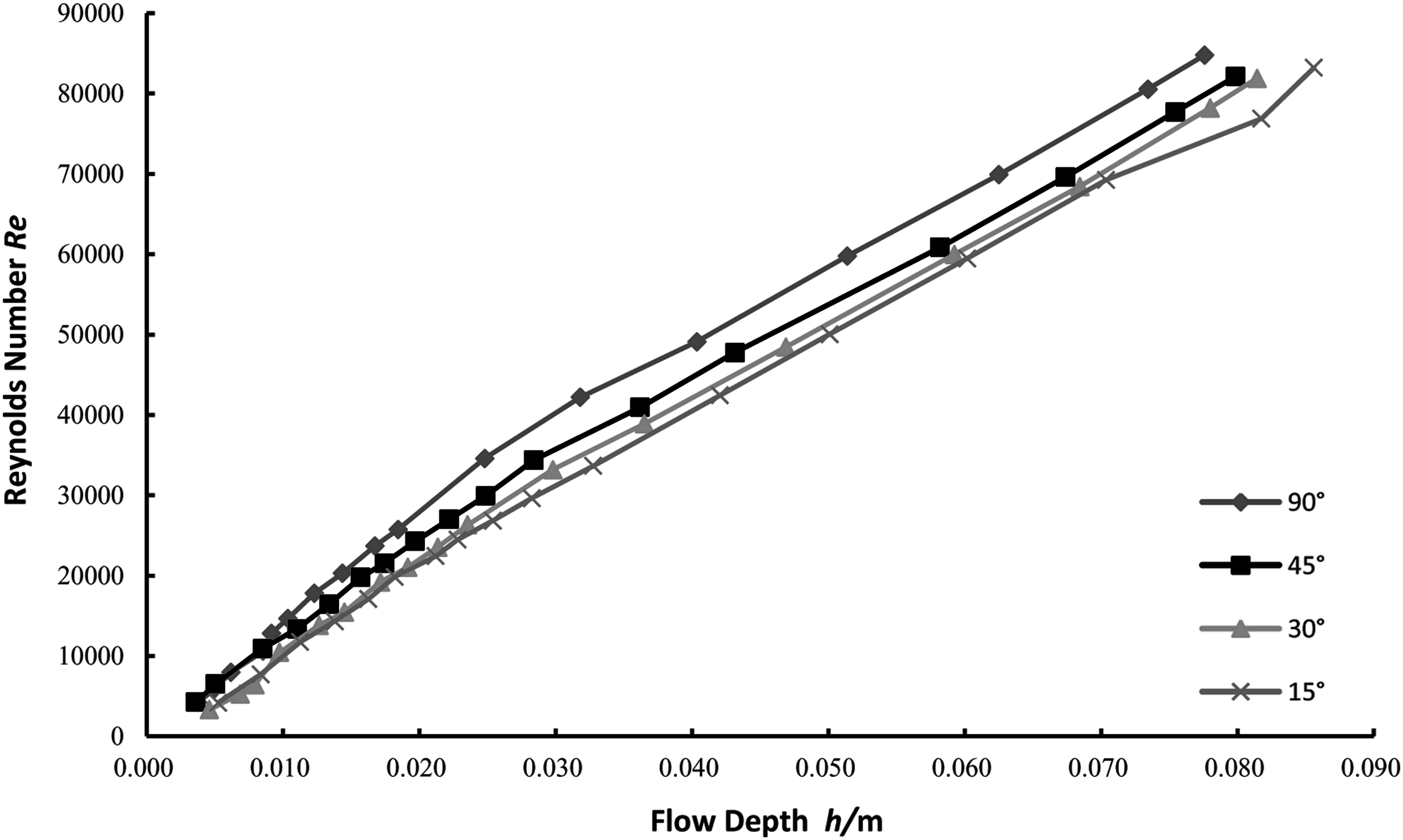
Diagram of the relationship between flow depth (h) and Reynolds number (Re). The four relationship curves in the figure represent the change of Re with h for the partially submerged conditions of four different vegetation distribution trend angles.

FIG. 5.

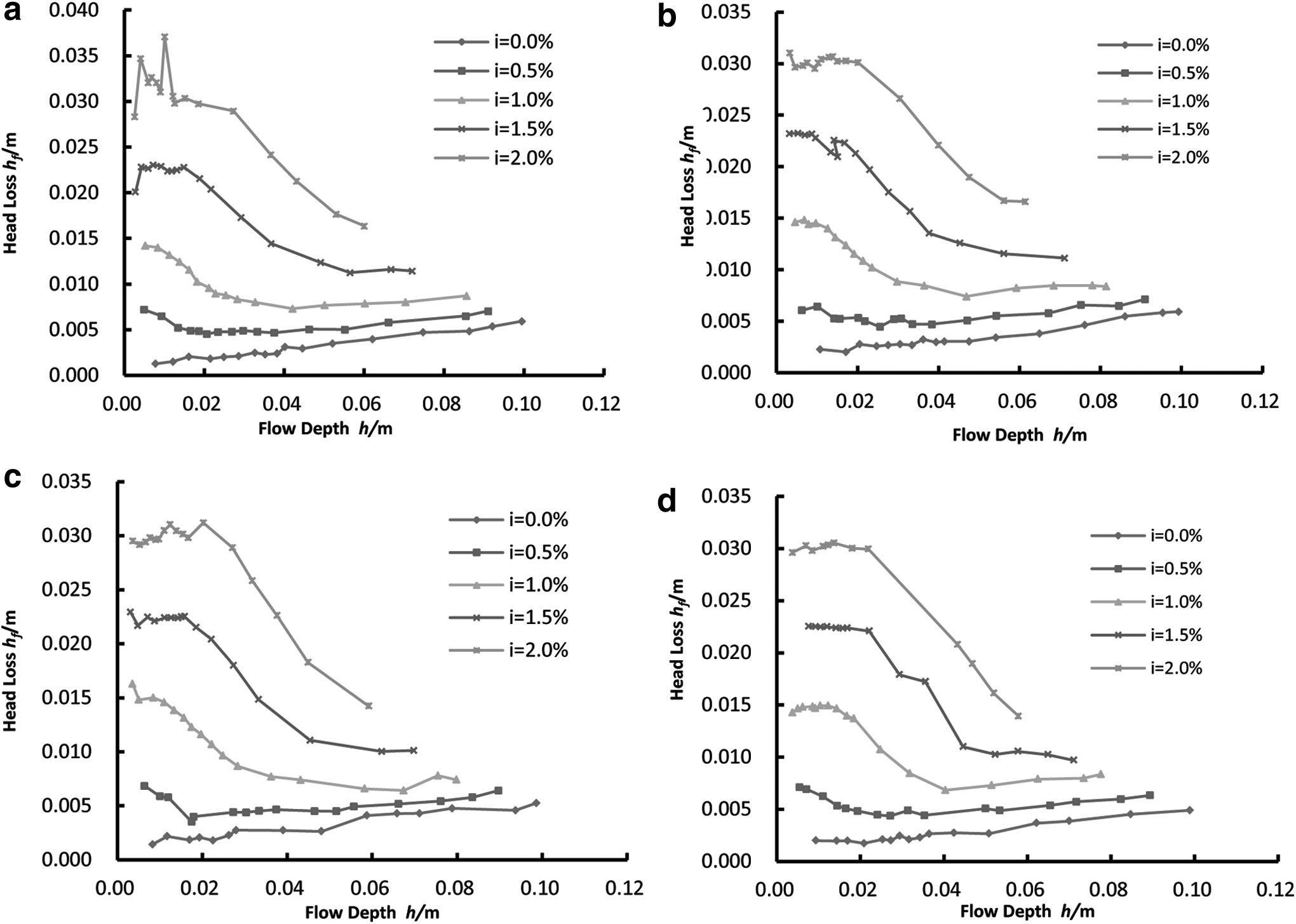
Diagram of the relationship between flow depth (h) and head loss (h_f). The four diagrams represent the relationship between the hydraulic changes of h and h_f for different slopes of four different vegetation distribution trend angles (θ). (a) θ = 15°, (b) θ = 30°, (c) θ = 45°, and (d) θ = 90°.

It can be seen from Fig. 4 that the angle between the vegetation row and the water flow direction angle (θ) influences the water flow state. At the same water depth, the larger the θ, the larger the Reynolds number. That is, when the angle between the vegetation row and the water flow direction is larger, the water flow is in a highly turbulent state when it flows through the vegetation. The smaller the angle between the vegetation row and the water flow direction, the weaker the turbulence state when the water flows through the vegetation. In addition, the difference of Re values corresponding to different θ is not constant. The less the submerged depth, the smaller the Re value. As the water depth increases, the Re value varies more and more. Figure 5 illustrates the data for partially submerged vegetation in all distributions, in which the water head loss increases as the slope becomes steeper for the same submergence condition. Meanwhile, the water head loss of flow through partially submerged vegetation is related to submergence, despite the angles between flow direction and vegetation distribution direction. When the gradient is nearly 0.0%, head loss increases with submergence. As the slope increases, head loss of flow through partially submerged vegetation will initially decrease, then reach a minimum value, and eventually slowly increase with increasing water depth.

Discussion

Further analysis of the resistance relationship revealed that when the vegetation distribution density is equal to that of the water depth, the resistance coefficient satisfies the following relationship: f_15° > f_30° > f_45° > f_90°. The resistance coefficient represents the resistance of the solid boundary to the water flow. If the submerged depth h is the same, the area of the solid boundary surface in contact with the water flow in the experiment is the same and the type of material is the same. In fact, in our experiment, we varied the angle (θ) of the vegetation distribution in the flow direction, thus changing the projected area of plants in the plane of vertical flow. Therefore, we can conclude that the variation of θ changes the vegetation projection width (K) on a plane that is vertical relative to the flow direction. K represents the flow cross-sectional area occupied by plant stems at a certain θ. Our data indicate that K varies with the change of θ, and can be represented by the following formula: \documentclass{aastex}\usepackage{amsbsy}\usepackage{amsfonts}\usepackage{amssymb}\usepackage{bm}\usepackage{mathrsfs}\usepackage{pifont}\usepackage{stmaryrd}\usepackage{textcomp}\usepackage{portland, xspace}\usepackage{amsmath, amsxtra}\usepackage{upgreek}\pagestyle{empty}\DeclareMathSizes{10}{9}{7}{6}\begin{document} \begin{align*} K = \frac { B } { { M \sin \theta } } d \tag { 11 } \end{align*} \end{document}

In this formula, K is the projection width of the plant stem; B is the flume width; M is the spacing between the plants; d is the plant stem width; and θ represents the angle of the flow direction and the vegetation distribution direction. In this experiment, d, M, and B were set as 3, 60, and 400 mm, respectively; θ had four values: 15°, 30°, 45°, and 90°; and K varied with θ (Table 3). The regression analysis of K and α is shown in Fig. 6.

FIG. 6.

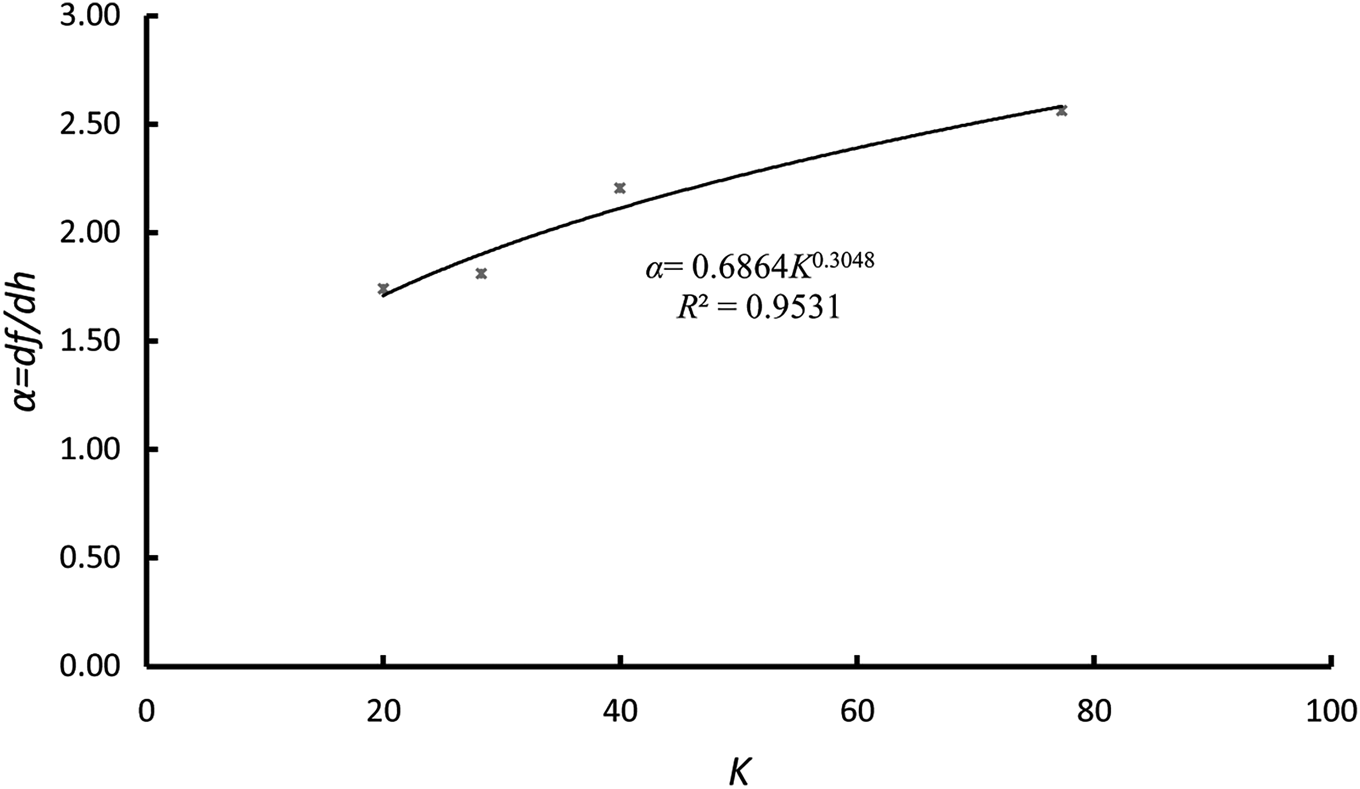
Diagram of the relationship between projection width K and the Darcy-Weisbach friction factor (f) change rate α in the partially submerged state. The abscissa is K, and the ordinate is α.

Table 3.

Parameters for Different Flow Directions and Partially Submerged Vegetation Row Angles

Angle, θ	Number of trails	Regression equations \documentclass{aastex}\usepackage{amsbsy}\usepackage{amsfonts}\usepackage{amssymb}\usepackage{bm}\usepackage{mathrsfs}\usepackage{pifont}\usepackage{stmaryrd}\usepackage{textcomp}\usepackage{portland, xspace}\usepackage{amsmath, amsxtra}\usepackage{upgreek}\pagestyle{empty}\DeclareMathSizes{10}{9}{7}{6}\begin{document} $$\textbf{\textit{f}} = \alpha h + \beta$$ \end{document}		Plant stems projector width, K/mm
Angle, θ	Number of trails	\documentclass{aastex}\usepackage{amsbsy}\usepackage{amsfonts}\usepackage{amssymb}\usepackage{bm}\usepackage{mathrsfs}\usepackage{pifont}\usepackage{stmaryrd}\usepackage{textcomp}\usepackage{portland, xspace}\usepackage{amsmath, amsxtra}\usepackage{upgreek}\pagestyle{empty}\DeclareMathSizes{10}{9}{7}{6}\begin{document} $$\alpha$$ \end{document}	β	Plant stems projector width, K/mm
15°	82	2.560	0.050	20.00
30°	85	2.203	0.080	28.29
45°	82	1.809	0.066	40.00
90°	72	1.739	0.063	77.28

Figure 6 illustrates the noteworthy power function between the change rate (α) of resistance coefficient (f) due to flow depth (h) and the width of the plant stem on a plane that is vertical to the flow direction (K), considering the resistance coefficient as a flow resistance representation of partially submerged vegetation. Thus, for the same flow and vegetation condition, the change of θ leads to resistance coefficient (f) variation, meaning that the flow resistance of partially submerged vegetation varies with flow direction and can be represented by the formula: \documentclass{aastex}\usepackage{amsbsy}\usepackage{amsfonts}\usepackage{amssymb}\usepackage{bm}\usepackage{mathrsfs}\usepackage{pifont}\usepackage{stmaryrd}\usepackage{textcomp}\usepackage{portland, xspace}\usepackage{amsmath, amsxtra}\usepackage{upgreek}\pagestyle{empty}\DeclareMathSizes{10}{9}{7}{6}\begin{document} \begin{align*} { \frac { df } { dh } } = 0.686 { K^ { 0.304 } } \tag { 12 } \end{align*} \end{document}

For the relationship between water depth and flow regime, the dimensionless parameter Reynolds number can be thought of in terms of the ratios of inertia force to viscous force acting on the water flow (Zheng et al., 2012). It can be said that the variation of θ changes the mechanical characteristics of the flow field. A large angle between the flow direction and vegetation distribution direction increases the ratio of the inertia force and viscous force in the flow field. At the same flow depth, the inertia force of water flow with a larger θ is greater than the inertia force of water flow with a smaller θ. The water flow with a larger θ tends to maintain the inertia movement. For the flow field with a smaller θ, the ratio of inertia force to viscous force decreases, and the viscous force is greater than that of the water flow with a larger θ. In this case, the water requires more energy to offset the viscous force effect, and energy consumption increases correspondingly. Therefore, at the same flow depth, the water flow with a smaller θ has a relatively large Darcy-Weisbach resistance coefficient. There is a demarcation point for head loss with changing water depth. At first, head loss (h_f) decreases with increasing water depth. Once the water depth has exceeded the demarcation point, the head loss (h_f) begins to slowly increase with increasing water depth. In addition, this demarcation point is not affected by the slope or vegetation distribution. It can be concluded that for partially submerged vegetation, the water flow is initially dominated by inertia forces, and the energy loss of water (represented by head loss) decreases rapidly with increasing submergence depth. When the flow rate increases slowly, the water layer becomes thicker, the gravitational potential energy of the water flow increases, and the water body energy loss increases slowly with water depth.

Conclusions

Variations in vegetation distribution direction influence the flood flow velocity and volume distribution by changing flow resistance. Although the vegetation distribution effect on flood flow resistance has previously been investigated, it still requires experimental verification. Our research simulated earth surface vegetation distribution directions by building a hydraulic model of an open channel, and investigated the effect of various vegetation distribution directions on flood flow resistance. Our findings can be summarized as follows.

(1)

For the same vegetation distribution trend angle, the relationship between the submerged water depth h and the resistance coefficient f at different slopes is constant, indicating that the slope change has no significant effect on the resistance coefficient f.

(2)

The resistance coefficient f is linearly proportional to the vegetation submerged depth h and has the basic form \documentclass{aastex}\usepackage{amsbsy}\usepackage{amsfonts}\usepackage{amssymb}\usepackage{bm}\usepackage{mathrsfs}\usepackage{pifont}\usepackage{stmaryrd}\usepackage{textcomp}\usepackage{portland, xspace}\usepackage{amsmath, amsxtra}\usepackage{upgreek}\pagestyle{empty}\DeclareMathSizes{10}{9}{7}{6}\begin{document} $$f = \alpha h + \beta$$ \end{document} . It can be concluded from the fitted linear equation that the change in the angle θ between the vegetation distribution trend and the water flow direction affects the rate of change \documentclass{aastex}\usepackage{amsbsy}\usepackage{amsfonts}\usepackage{amssymb}\usepackage{bm}\usepackage{mathrsfs}\usepackage{pifont}\usepackage{stmaryrd}\usepackage{textcomp}\usepackage{portland, xspace}\usepackage{amsmath, amsxtra}\usepackage{upgreek}\pagestyle{empty}\DeclareMathSizes{10}{9}{7}{6}\begin{document} $$\alpha$$ \end{document} of the resistance coefficient f. That is, the smaller the value of θ, the larger the rate of change \documentclass{aastex}\usepackage{amsbsy}\usepackage{amsfonts}\usepackage{amssymb}\usepackage{bm}\usepackage{mathrsfs}\usepackage{pifont}\usepackage{stmaryrd}\usepackage{textcomp}\usepackage{portland, xspace}\usepackage{amsmath, amsxtra}\usepackage{upgreek}\pagestyle{empty}\DeclareMathSizes{10}{9}{7}{6}\begin{document} $$\alpha$$ \end{document} . However, the larger the value of θ, the smaller the rate of change \documentclass{aastex}\usepackage{amsbsy}\usepackage{amsfonts}\usepackage{amssymb}\usepackage{bm}\usepackage{mathrsfs}\usepackage{pifont}\usepackage{stmaryrd}\usepackage{textcomp}\usepackage{portland, xspace}\usepackage{amsmath, amsxtra}\usepackage{upgreek}\pagestyle{empty}\DeclareMathSizes{10}{9}{7}{6}\begin{document} $$\alpha$$ \end{document} .

(3)

The change of the angle θ between the vegetation distribution trend and the water flow direction affects the projection width K of the vegetation perpendicular to the flow direction plane. Our experiments revealed that the rate of change \documentclass{aastex}\usepackage{amsbsy}\usepackage{amsfonts}\usepackage{amssymb}\usepackage{bm}\usepackage{mathrsfs}\usepackage{pifont}\usepackage{stmaryrd}\usepackage{textcomp}\usepackage{portland, xspace}\usepackage{amsmath, amsxtra}\usepackage{upgreek}\pagestyle{empty}\DeclareMathSizes{10}{9}{7}{6}\begin{document} $$\alpha$$ \end{document} of the resistance coefficient f with the vegetation at submerged depth h and the vegetation projection width K satisfy a certain functional relationship. That is to say, varying vegetation distribution trends cause the projection width K to change, which alters the change rate \documentclass{aastex}\usepackage{amsbsy}\usepackage{amsfonts}\usepackage{amssymb}\usepackage{bm}\usepackage{mathrsfs}\usepackage{pifont}\usepackage{stmaryrd}\usepackage{textcomp}\usepackage{portland, xspace}\usepackage{amsmath, amsxtra}\usepackage{upgreek}\pagestyle{empty}\DeclareMathSizes{10}{9}{7}{6}\begin{document} $$\alpha$$ \end{document} , finally leading to the differential change of the resistance coefficient f.

(4)

Our experiments prove that the vegetation distribution trend has an anisotropic effect on the turbulence degree of the water flow in different flow directions. At the same water depth, when the vegetation distribution trend angle θ is larger, the larger the corresponding Reynolds number and the higher the water flow turbulence degree. When the water depth is shallow, the difference in turbulence between different flow directions is small. As the water depth increases, the difference in turbulence between different flow directions increases.

(5)

There is a demarcation point in the process of energy loss change. Before the demarcation point of water depth, the head loss decreases with increasing water depth; after the demarcation point, it increases slowly as the water depth increases. This indicates that the inertia force is dominant at the beginning of the water flow. After the demarcation point, the water layer is thickened, and gravitational potential energy drives the water flow.

Footnotes

Acknowledgments

We would like to thank the National Natural Science Foundation of China (Grant No. 41471025), the Natural Science Foundation of Shandong Province (Grant No. ZR2014DM004), and the Major Research and Development Program of Shandong Province (Grant Nos. 2016GSF117027 and 2016GSF117036) for supporting this project.

Author Disclosure Statement

No competing financial interests exist.

References

Abrahams

A.D.

, Parsons

A.J.

, and Wainwright

(1994). Resistance to overland flow on semiarid grassland and shrubland hillslopes, Walnut Gulch, Southern Arizona. J. Hydrol. 156, 431.

Arguelles

A.C.

, Jung

, and Pak

(2013). Evaluation of overland flow model for a hillslope using laboratory flume data. Water Sci. Technol. 68, 1188.

Chen

, Liu

X.N.

, and Wang

X.K.

(2015). Effects of roughness elements distribution on overland flow resistance. J. Mt. Sci. Engl. 12, 1145.

Cheng

N.S.

(2011). Representative roughness height of submerged vegetation. Water Resour. Res. 47, 1.

Cheng

N.S.

, and Nguyen

H.T.

(2011). Hydraulic radius for evaluating resistance induced by simulated emergent vegetation in open-channel flows. J. Hydraul. Eng. 137, 995.

Cooper

J.R.

, Tait

S.J.

, and Horoshenkov

K.V.

(2006). Determining hydraulic resistance in gravel-bed rivers from the dynamics of their water surfaces. Earth Surf. Proc. Land. 31, 1839.

Cristo

D.C.

, Michele

, and Andrea

(2012). Green's function of the linearized saint-venant equations in laminar and turbulent flows. Acta Geophys. 60, 173.

Ding

W.F.

, and Li

(2016). Effects of grass coverage and distribution patterns on erosion and overland flow hydraulic characteristics. Environ. Earth Sci. 75, 1.

Duan

L.X.

, Huang

M.B.

, and Zhang

L.D.

(2016). Differences in hydrological responses for different vegetation types on a steep slope on the Loess Plateau, China. J. Hydrol. 537, 356.

10.

Fraga

, Cea

, and Puertas

(2013). Experimental study of the water depth and rainfall intensity effects on the bed roughness coefficient used in distributed urban drainage models. J. Hydrol. 505, 266.

11.

Guo

J.Y.

, Sun

J.L.

, and Chang

X.T.

(2011). Correlation Analysis of NINO3.4 SST and inland lake level variations monitored with satellite altimetry: Case studies of Lakes Hongze, Khanka, La-ang, Ulungur, Issyk-kul and Baikal. Terr. Atmos. Ocean. Sci. 22, 203.

12.

Järvelä

(2004). Determination of flow resistance caused by non-submerged woody vegetation. Int. J. River Basin Manag. 2, 61.

13.

Järvelä

(2005). Effect of submerged flexible vegetation on flow structure and resistance. J. Hydrol. 307, 233.

14.

Kadlec

R.H.

(1990). Overland flow in wetlands: Vegetation resistance. J. Hydraul. Eng. 116, 691.

15.

Kim

, Ivanov

V.Y.

, and Katopodes

N.D.

(2012). Hydraulic resistance to overland flow on surfaces with partially submerged vegetation. Water Resour. Res. 48, 10540.

16.

Laounia

, Yan

Z.M.

, and Xia

J.H.

(2005). Study of the flow through non-submerged vegetation. J. Hydrodyn. 17, 498.

17.

Liu

, Xu

, and Zhou

(2018). Relation between crack propagation and internal damage in sandstone during shear failure. J. Geophys. Eng. 15, 2104.

18.

Liu

, Yasufuku

, and Omine

(2018). Self-watering system for arid area: A method to combat desertification. Soils Found. 58, 838.

19.

Liu

X.R.

, Shen

Y.J.

, and Guo

(2010). Modeling demand/supply of water resources in the arid region of northwestern China during the late 1980s to 2010. J Geogr. Sci. 25, 573.

20.

Luhar

, and Nepf

H.M.

(2013). From the blade scale to the reach scale: A characterization of aquatic vegetative drag. Adv. Water Resour., 51, 305.

21.

Luhar

, Rominger

, and Nepf

(2008). Interaction between flow, transport and vegetation spatial structure. Environ. Fluid Mech. 8, 423.

22.

Neary

V. S.

, Constantinescu

S.G.

, and Bennett

S.J.

(2012). Effects of vegetation on turbulence, sediment transport, and stream morphology. J. Hydraul. Eng. 138, 765.

23.

Nepf

H.M.

(1999). Drag, turbulence, and diffusion in flow through emergent vegetation. Water Resour. Res. 35, 1985.

24.

Noarayanan

, Murali

, and Sundar

(2012). Manning's “n” co-efficient for flexible emergent vegetation in tandem configuration. J. Hydro Environ. Res. 6, 51.

25.

Okamoto

T.A.

, Nezu

, and Ikeda

(2012). Vertical mass and momentum transport in open-channel flows with submerged vegetations. J. Hydro Environ. Res. 6, 287.

26.

Roche

, Daıän

J.F.

, and Lawrence

D.S.L.

(2007). Hydraulic modeling of runoff over a rough surfaceunder partial inundation. Water Resour. Res. 43, 8410.

27.

Sedghi-Asl

, and Rahimi

(2011). Adoption of Manning's equation to 1D non-Darcy flow problems. J. Hydraul. Res. 49, 814.

28.

Stephan

, and Gutknecht

(2002). Hydraulic resistance of submerged flexible vegetation. J. Hydrol. 269, 27.

29.

Stone

B.M.

, and Shen

H.T.

(2002). Hydraulic resistance of flow in channels with cylindrical roughness. J. Hydraul. Eng. 128, 500.

30.

Tang

H.W.

, Tian

Z.J.

, Yan

, and Yuan

S.Y.

(2014). Determining drag coefficients and their application in modelling of turbulent flow with submerged vegetation. Adv. Water Resour. 69, 134.

31.

Wang

, Zhang

, and Qiu

Y.B.

(2015). Snow effects on alpine vegetation in the Qinghai-Tibetan Plateau. Int. J. Digit. Earth, 8, 56.

32.

F.C.

, Shen

H.W.

, and Chou

Y.J.

(1999). Variation of roughness coefficients for unsubmerged and submerged vegetation. J. Hydraul. Eng. 125, 934.

33.

L.H.

, and Yang

X.L.

(2014). Influence of bending rigidity of submerged vegetation on local flow resistance. J. Hydrodyn. 26, 242.

34.

Yagci

, Tschiesche

, and Kabdasli

M.S.

(2010). The role of different forms of natural riparian vegetation on turbulence and kinetic energy characteristics. Adv. Water Resour. 33, 601.

35.

Yen

B.C.

(2002). Open channel flow resistance. J. Hydraul. Eng. 128, 20.

36.

Zhang

, Liu

, and Wang

(2012). Effects of patterned Artemisia capillaries on overland flow velocity under simulated rainfall. Hydrol. Process. 26, 3779.

37.

Zhang

S.T.

, Liu

Y.C.

, and Zhang

J.Z.

(2018). Study of the impact of vegetation direction and slope on drag coefficient. IJST. T. Civ. Eng. 42, 381.

38.

Zheng

Z.C.

, He

S.Q.

, and Wu

F.Q.

(2012). Relationship between soil surface roughness and hydraulic roughness coefficient on sloping farmland. Water Sci. Eng. 5, 191.