Dispersion of Pollutants in a River According to Its Geometry and Tributaries: A Case Study for River Paraiba do Sul

Abstract

This article aims to demonstrate how the dispersion of pollution is affected when the main flow of river changes due to river geometry also with inflows coming from tributaries. The river chosen is Paraiba do Sul because it flows through two important states in Brazil, Rio de Janeiro and Sao Paulo, and supplies water for several purposes, such as agriculture, drinking, energy, dissolution of domestic sewage, fishing, and so on. Through a single two-dimensional numerical simulation (Computational Fluid Mechanics—CFD) by commercial software COMSOL Multiphysics, it was possible to demonstrate how geometry of a river and tributaries' inflow rates changes the dispersion of pollutants along its course.

Introduction

The study of flow and transport of chemical products into fluids is of fundamental importance in several areas of engineering, including Environmental Engineering. Among fluids focused on in Environmental studies, water and possible ways to feed it efficiently and within usable quality standard are of essential importance for the environment and population. To benefit populations, it is globally accepted that drinkable water is a scarce but available resource, which justifies the search for ways to feed it in an efficient manner and to be able to reach a wide range of places/people (Lenzen et al., 2013). Ultimately, drinkable water is the major source for human health and survival.

Localized in the Southeast of Brazil, Paraiba do Sul River is composed of the inflows of two rivers, Paraibuna and Paraitinga, both born in Bocaina Sierra, in the cities of Cunha and Areias. The Paraiba do Sul River has a sinuous profile stream that goes from the eastern to the western parts of the country flowing parallel to and between the Mantiqueira sierra and Atlantic Ocean. After passing through part of State of Sao Paulo, Paraiba do Sul River heads to State of Rio de Janeiro flowing through a region called Vale do Paraiba, situated in State of Rio de Janeiro. Finally, Paraiba do Sul River trajectory ends up in the Atlantic Ocean after it has flowed for ∼1,150 km.

Due to the high number of inhabitants and industries in the region near the course of the river, which has been populated for decades, the necessity for clean water has become an important theme to be explored (Rosa, 2012). According to the same author, water from this river is used by the population and companies, to dilute sewage, irrigate crops, generate hydroelectric energy, and, on minor scale, for fishing, agriculture, recreation, and sailing. To have an idea of the magnitude of water consumption, the transposition of the river to generate hydro energy consumes approximately two-thirds of the total flow of water in State of Sao Paulo. In addition, it consumes 100% of one of its tributaries called Pirai River.

There are several simulations produced worldwide that study numerically the dispersion of pollutants in rivers, streams, and seas; most of them highlight how harmful the pollutants are for the society's health.

Among the simulations, Leo and Seo (2010) is an example that shows a numerical model, which replicates situations where the disposal of pollutants happens due to accident. In addition, they demonstrate the reliability of their model stating that it can also be used for other similar studies. Similar to Leo and Seo (2009) work, when they studied a portion of the River Han in Korea, this article uses the finite element method to simulate dispersion of pollutants.

In addition Seo, et al. (2016), using software RAM, presented the results of a two-dimensional (2D) simulation of River Sum. In their study, they monitored six points along the river, from which a few data such as volumetric flow, velocity of stream, and other information are collected. Similar to this article, Seo et al. (2016) also measured the concentration of pollutants within few time intervals.

Water is known as an essential element for human survival, especially pure water, which is a scarce substance as no more than 1% of the total volume is available for consumption. Therefore, the quality of water, mainly of rivers and their springs, is of extreme importance to preserve species and human lives.

In this sense, Halaj et al. (2014) simulate numerically under one-dimensional and 2D the River Ondave (422 m length) aiming to find alternatives to obtain a better quality of water. With their simulation, they brought a few proposals to enhance the quality of water.

In addition to the references previously described, there are several other authors like Petrescu and Sumbasacu (2010), Tsanis and Boyle (2001), Belcaid et al. (2012), and Andrei (2011) who study pollutant dispersion in rivers aiming to obtain enough knowledge and improve the quality of water. Therefore, this article aims to demonstrate how the dispersion of pollution is affected when the main flow of river changes due to river geometry, as well as inflows coming from tributaries. In addition, this work contributes to enhance the knowledge of dispersion of pollutants in rivers using numerical simulation, particularly by finite element methods.

Methodology

Model equation

Here is a numerical study of a differential partial equation that models the flow phenomena in two directions. The equation is known as Navier–Stokes equation (Arpaci, 1966; Bejan, 1996): $\frac{\partial u}{\partial x} + \frac{\partial v}{\partial y} = 0$ (1) $ρ (\frac{\partial u}{\partial t} + u \frac{\partial u}{\partial x} + v \frac{\partial u}{\partial y}) = - \frac{\partial p}{\partial x} + μ (\frac{\partial^{2} u}{\partial x^{2}} + \frac{\partial^{2} u}{\partial y^{2}}) + X$ (2)

ρ (\frac{\partial v}{\partial t} + u \frac{\partial v}{\partial x} + v \frac{\partial v}{\partial y}) = - \frac{\partial p}{\partial y} + μ (\frac{\partial^{2} v}{\partial x^{2}} + \frac{\partial^{2} v}{\partial y^{2}}) + Y

(3)

Equation (1) is known as an equation of continuity equation, Equations (2) and (3) are known as the momentum equations in the directions x and y, ρ is the density (kg/m³), μ is dynamic viscosity (kg/[m·s]), u and v are the components of velocity (m/s) in the directions x and y, p is the pressure (N/m²), and finally X and Y are the forces of field in directions x and y, respectively.

Beyond Equations (1)–(3) the equation of conservation of concentration is used as follows: $\frac{\partial C_{A}}{\partial t} + u \frac{\partial C_{A}}{\partial x} + v \frac{\partial C_{A}}{\partial y} = D_{A B} (\frac{\partial^{2} C_{A}}{\partial x^{2}} + \frac{\partial^{2} C_{A}}{\partial y^{2}}) + N_{A}$ (4)

for C_A as the concentration (of a pollutant, e.g.), N_A is flow molar, and $D_{A B}$ is the binary diffusion coefficient (which represents the capacity of chemical specie A to diffuse in chemical specie B in m²/s). It is important to reinforce that a chemical specie is conserved not its concentration.

To create a 2D model for numerical simulation, Google Earth was utilized as a dimensional reference (Figs. 1 and 2) and AutoCAD as a tool to produce the 2D drawing of the profile of Paraiba do Sul River. With the model finished, it was transferred to a Computational Fluid Dynamics (CFD) model in the COMSOL Multiphysics software. This software solved the equations necessary for the study of flow and the dispersion of chemicals.

FIG. 1.

Overview of Sao Paulo and Rio de Janeiro provinces with localization of Paraiba do Sul River.

FIG. 2.

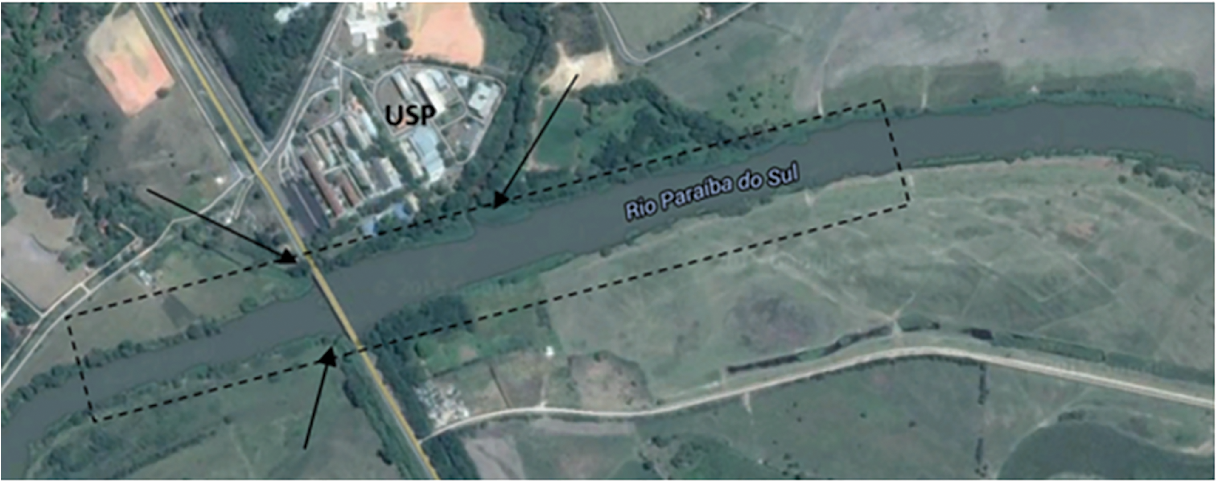
A closer look at Paraiba do Sul River showing a few tributaries.

This study focused on 6 km of the river's length, starting at Ep (Entrance Pollution) and ending at point S (Fig. 3, left). The river has tributary inflows labeled from 1 to 4 along the river trajectory. To measure the influence of the inflows in the water concentration of the river mainstream, six measurement points were determined (A, B, C, D, E, and F), as seen in Fig. 4. The distribution of points for measurement aimed to know the change on the River mainstream water concentration before the tributary inflow and just after it. Point A, for example, is localized before the tributary 1, while point B just after it. Point C is just before the tributary 2 and 3; point D is at the transition of point 2 and 3, which means at the end of point 2 and beginning point 3. Already the point E is localized just after the tributary 3 because it can reveal the influence of both points 2 and 3 in the water concentration—pollutants—in the river mainstream. The measurement point F shows the amount of flow added in the mainstream just after final tributary number 4. In addition it shows the influence of all tributaries in the river mainstream water concentration. For this simulation pure water was selected because it represents partially the river—mainly because the water cleanliness was not measured for this study—in contrast, pure water can clearly reveal the influence of other variables in the river mainstream pollutant level. It is important to make clear that the chemical condition of the river was not measured for this simulation. The points 2, 3, and 4 (Fig. 3, left) are in region shown in Fig. 2.

FIG. 3.

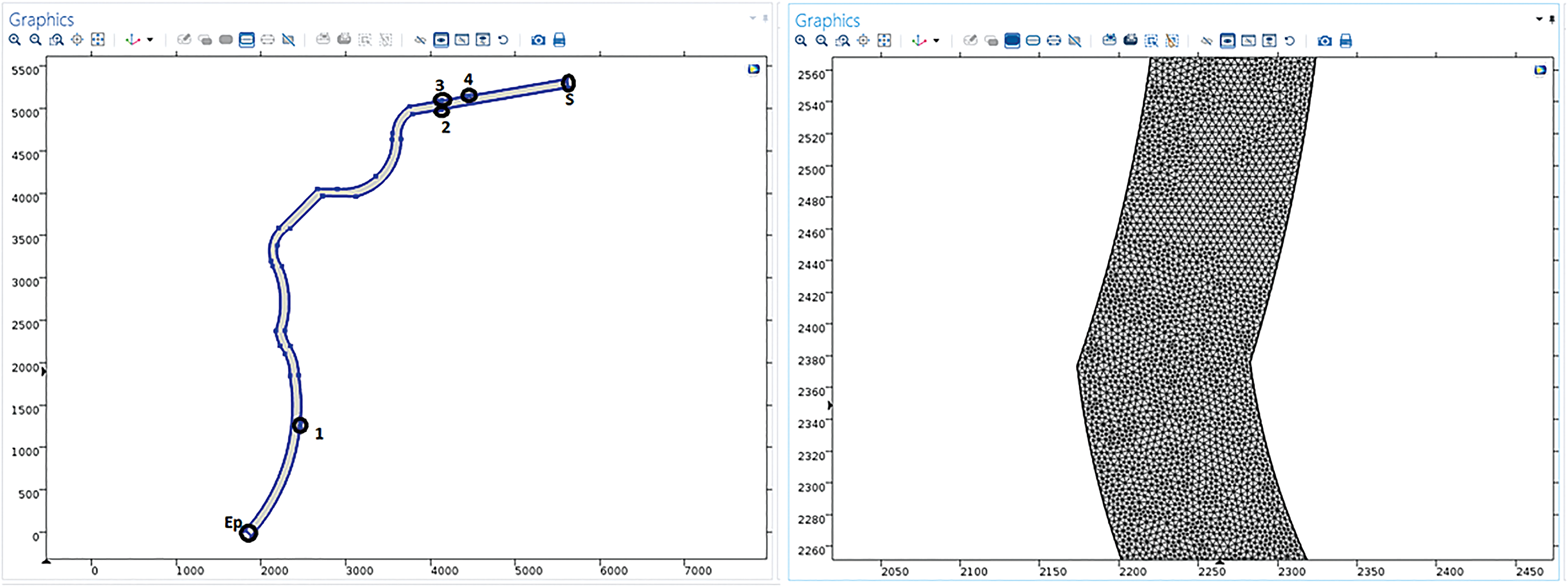
(Left) Domain imported from AutoCAD to COMSOL with tributaries labeled, (right) region of Paraiba do Sul River meshed 5 m (as larger element) in the domain.

FIG. 4.

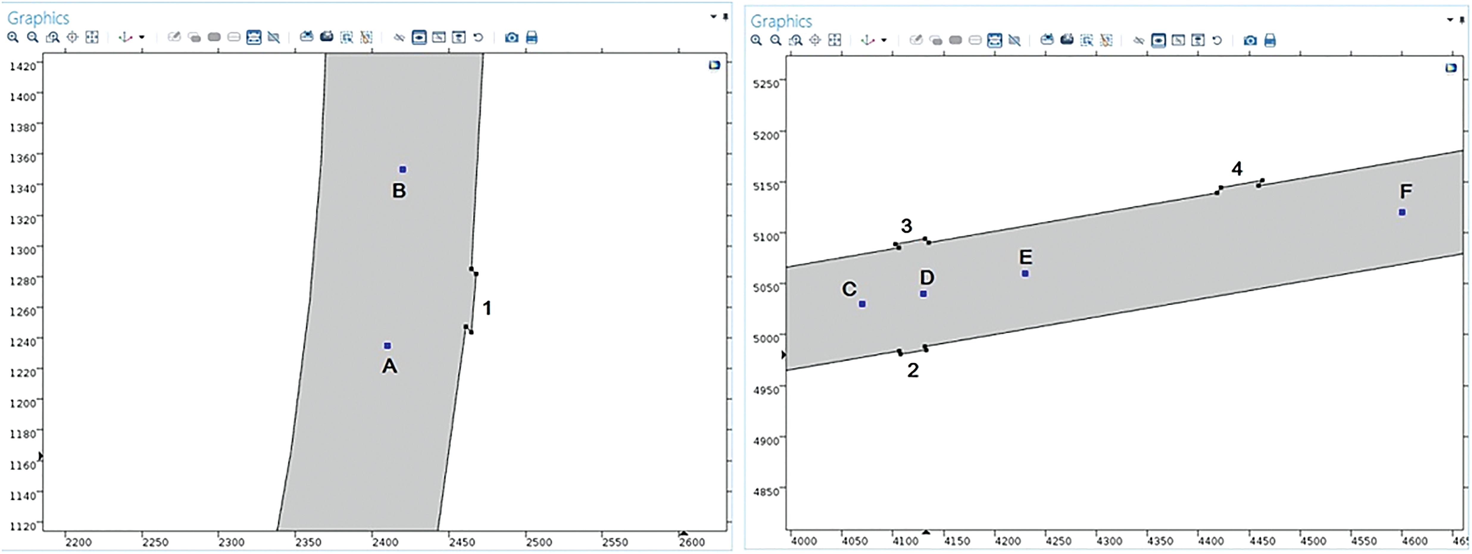
Points for measurement of velocity of water flow.

Numerical Application

Study of dispersion and absorption of nutrients

To have the velocities in the main stream of the river, a dry season was considered because the velocity of Paraiba do Sul River is slower at that time. The velocity for the main stream at Ep was chosen as 0.7 m/s, approximate values for the region between Pindamonhangaba city and Queluz city based on Marengo and Alves (2005). The velocity of affluenties at points 2, 3, and 4 was fixed at 0.12 m/s, while the velocity at affluent 1 (V1) had four variations 0.3, 0.6, 0.7, and 0.9 m/s. The tributaries 2, 3, and 4 are three narrow streams with normally clean water (Rosseti, 2009), and affluent 1 is the well-known Ribeirão Taboão that passes inside Lorena City.

For simulation purposes, COMSOL software module Transport of Diluted Species was utilized. An input required by COMSOL is a binary coefficient of diffusion for chemical specie studied, in m²/s. This value represents how easy it is for a solute to move throughout a solvent. Among the values found in the literature, the value for ammoniacal nitrogen was picked for this study. This substance indicates the presence of domestic sanitary sewage in water. An important characteristic of this chemical is that it is absorbed by aquatic plants, which helps in the process of depollution of rivers (Von Sperling, 1996). For this simulation, the value chosen as the binary coefficient for diffusion was 1.96 × 10⁻⁹ (m²/s) (Cremasco, 2002).

In addition, to define velocity and diffusion coefficients, it is necessary to determine a few parameters as follows: sources of pollution, the initial concentration of ammoniacal nitrogen, and the concentration of nitrogen already present in the main stream of river. The tributary 1 is chosen as having the highest concentration of sanitary sewage because this river flows through a populated city called Lorena—Sao Paulo. This city effuses a considerable amount of domestic sewage through several points along its entire route (Oliveira et al., 2018).

In regard to the initial concentration of ammoniacal nitrogen at tributary 1 the study by Oliveira et al. (2018) was referenced, and it classifies the sewage as medium pollution level with 25 mg/L (1.389 mol/m³) according to the same author, also as per Eddy (1991). For the value of concentration of ammoniacal nitrogen already present in the river it was considered 0.0277 mol/m³ [Companhia Ambiental do Estado de Sao Paulo (CETESB), 2018]. It is important to reinforce that the concentration in Ep is fixed in 0.0277 mol/m³ (boundary condition).

In addition, to approach a real problem, the entry of this pollutant into the tributary will not be constant; it is assumed as having a decrease over a period of time, thus the input concentration of the ammoniacal nitrogen is governed by the following equation [Eq. (5)]: $C_{e} = 1, 389 e^{- t}$ (5)

in which C_e is the concentration in mol/m³ of entry in affluent 1 and t is the time in s.

In terms of absorption of pollution by aquatic plants—called macrophyte—it was selected in the software and distributed along the river; this is because the absorption happens along the whole course of the river, also covering 20% of the area of river. It was considered that macrophyte absorbs 0.0002 kg of ammoniacal nitrogen per m² per day (Boschilia, 2014). As a consequence, the total absorption considered for the whole domain of the river was 2.153 × 10⁻⁷ mol/[m³·s].

Simulations were made for a total of 8,000 s, for intervals of 1 s each. The concentrations at points A, B, C, D, and E were recorded for times of 0, 100, 1,000, 2,000, 3,000, 4,000, 5,000, 6,000, 7,000, and 8,000 s. With those data collected, six graphs were generated and they show the variations of concentration (C) in mol/m³ with time. To see how the velocity of the tributaries influences the water concentration (at the measurement points), the graphs from Figs. 5–10 are used. These graphs show the water concentration for each variation of velocity for tributary 1 (V1) when it transfers pollutants to the river.

FIG. 5.

Graph of the variation of C (concentration) at point A over time t for each value of V1.

Analyzing the graph in Fig. 5, it is noticed that at point A the concentration decreases until t = 2,000 s and becomes constant due to the absorption of ammoniacal nitrogen. Immediately thereafter, between 2,000 and 3,000 s, the region enters in permanent regime where there is equilibrium between ammoniacal nitrogen and river water, mainly because the water of river is capable of absorbing the quantity of ammoniacal nitrogen coming from the entrance Ep that reaches the point A. Note that point A is before affluent 1.

In terms of concentration of ammoniacal nitrogen at Point B (Fig. 6), for all velocities, there is a proportional relationship between the increase in time and the lowering of the quantity of ammoniacal nitrogen disposed into the river as described in the Equation (6). Therefore, as the time increases the affluent 1 stops as a polluter and disposes water with lower and lower concentrations of pollutants into river. Beyond that, the river is wider than the tributary and it helps to disperse pollutants, which means no more increase of concentration at this point is verified.

FIG. 6.

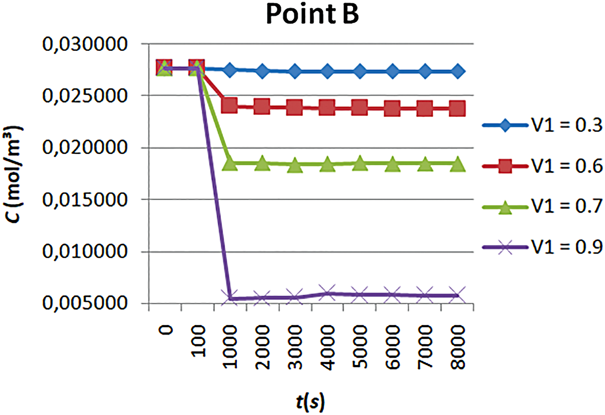
Graph of the variation of C (concentration) at point B over time t for each value of V1.

In addition, it is confirmed that the permanent regime is reached after 1,000 s for all velocities. Furthermore, it is observed that there is a difference in behavior between points C, D, E, and F (Figs. 7–10), localized closer to the end of the trajectory, compared with points A and B. In other words, the concentration of ammoniacal nitrogen decreases slowly, as a consequence of the absorption occurring along the river. From t = 4,000 s on, there is an influence of the entrance in the main stream (Ep) and tributary 1 for all velocities.

FIG. 7.

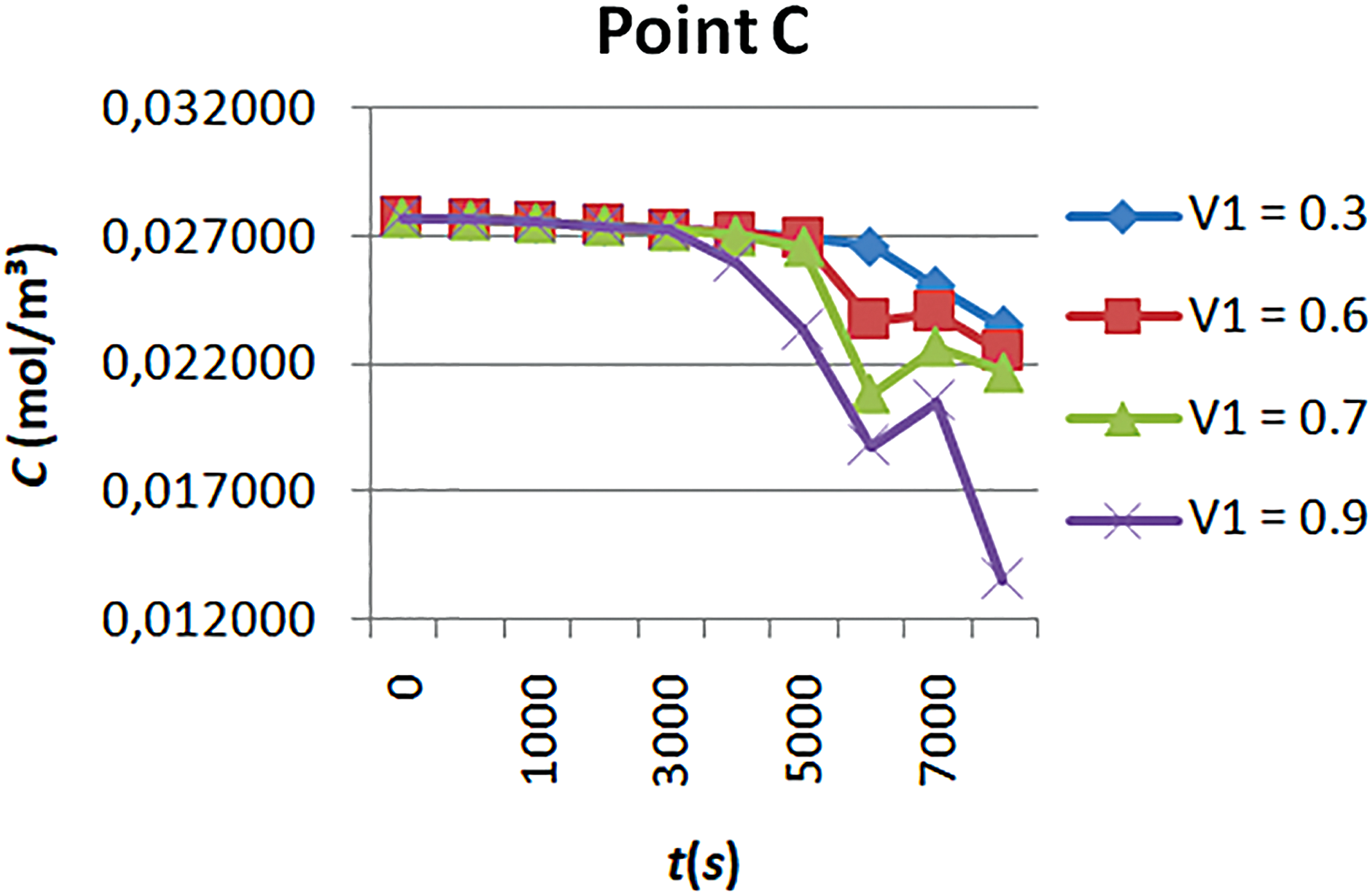
Graph of the variation of C (concentration) at point C over time t for each value of V1.

FIG. 8.

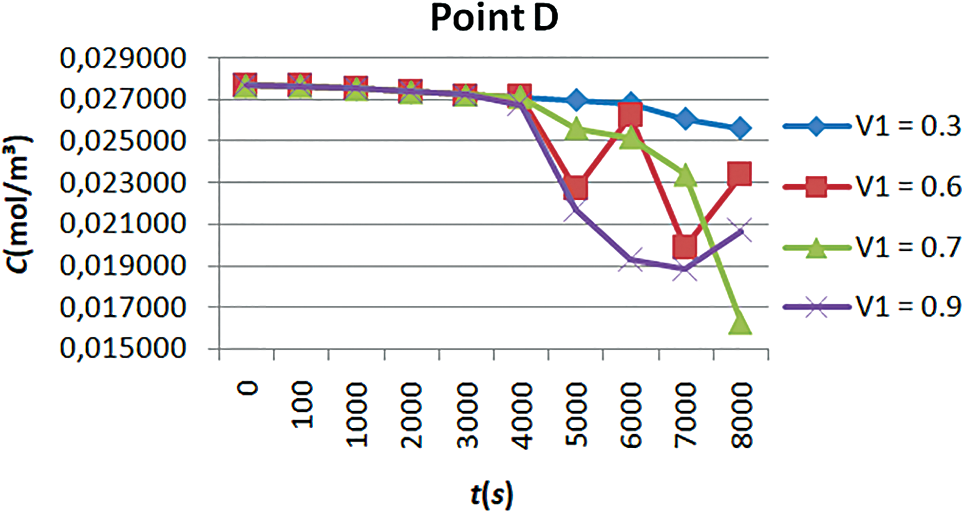
Graph of the variation of C (concentration) at point D over time t for each value of V1.

FIG. 9.

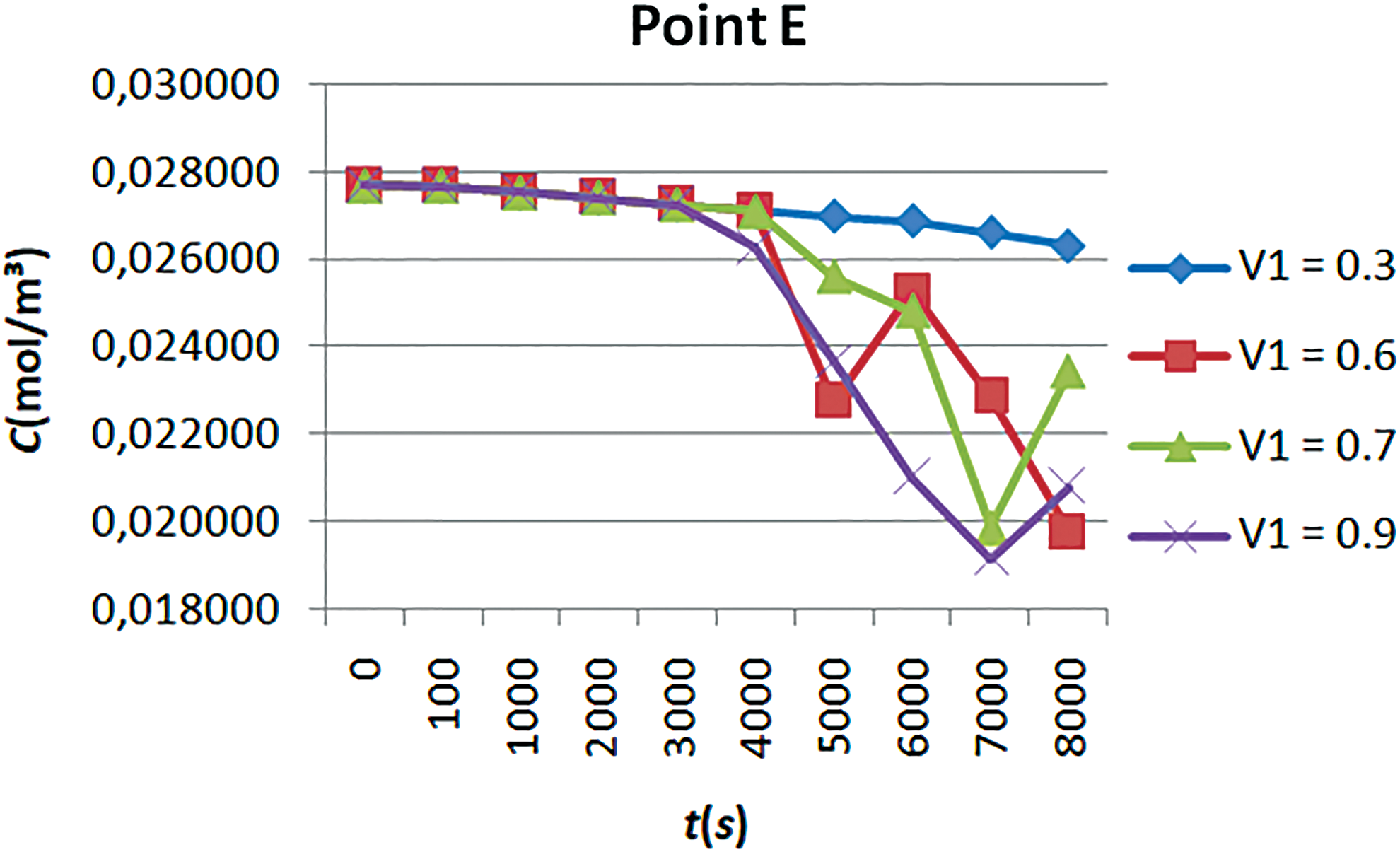
Graph of the variation of C (concentration) at point E over time t for each value of V1.

FIG. 10.

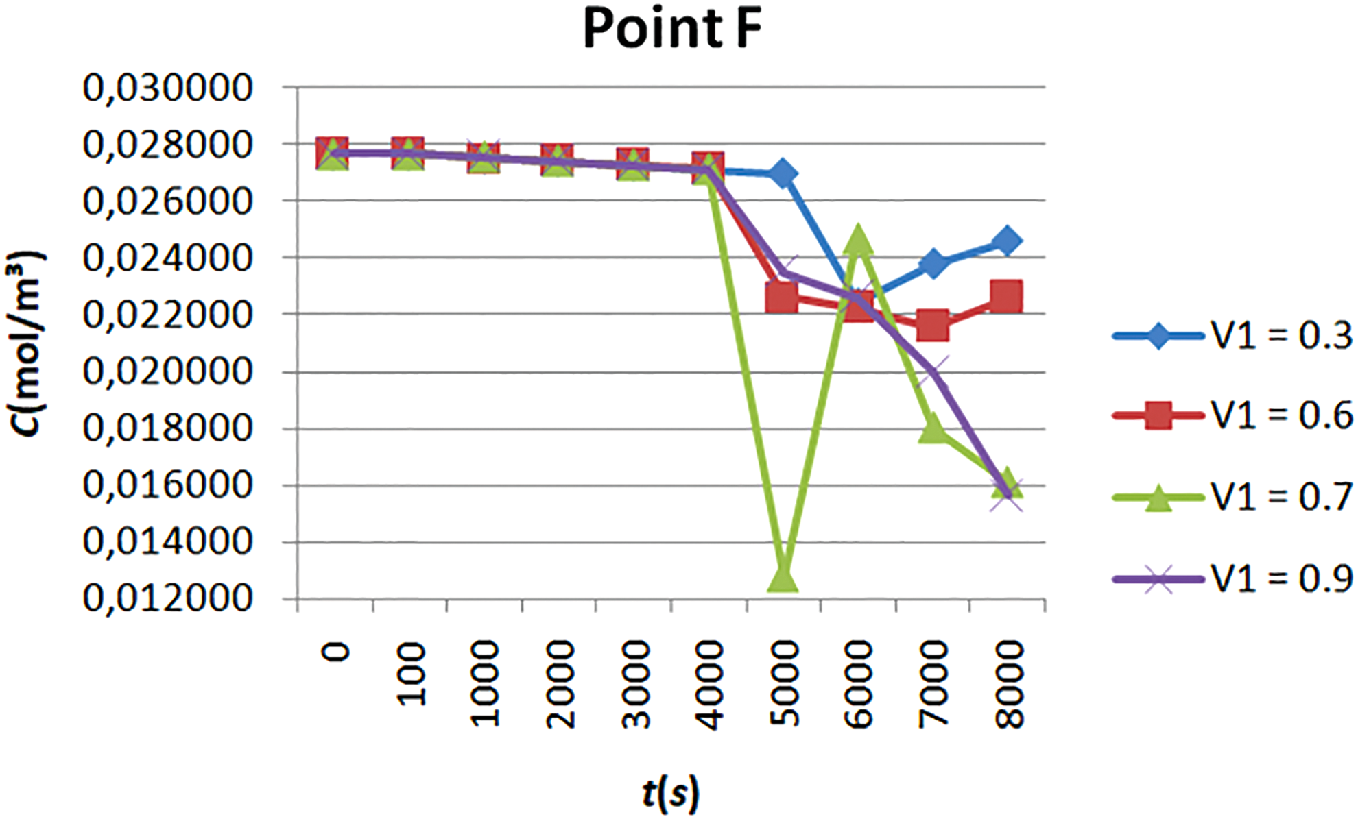
Graph of the variation of C (concentration) at point F over time t for each value of V1.

Figure 7 shows a decrease of the concentration of pollutants at point C and how the velocity of the disposal of the pollutants influences concentration; that is, a higher velocity of disposal from affluent 1 brings a lower concentration of ammoniacal nitrogen to the river. It is important to mention that because point C is before the tributary 2, 3, and 4, there is no influence of these affluents at point C.

At points D, E, and F, the concentrations in tributaries 2, 3, and 4 are zero (0 mol/m³), which means that only clean water is disposed into river. Figures 7–10 demonstrate a decrease in the concentration of ammoniacal nitrogen; however, it is not possible to claim that at these points there is a permanent regime established.

Conclusion

With the results obtained for the absorption and dispersion of pollutants, it is observed that the absorption by plants actually occurs, however, in a small scale. In addition, the change in velocity of tributary 1 varies the result of the ammoniacal nitrogen concentration at points B and C along the course of the river; as a matter of fact, higher velocities have higher influences on the output. In regard to the concentration of ammoniacal nitrogen, because of the disposal of tributary 1, the ammoniacal nitrogen rapidly diminishes with time along the course of the river. The large size of the river helps to assimilate chemical pollution. Nevertheless, the river has more than one unique tributary that disposes sewage into the river, which compromises the quality of the water. The next step is to combine several rates of absorption, concentrate pollutants, and dispose other chemical species along the river, striving to obtain results which are as close as possible to the reality.

Footnotes

Author Disclosure Statement

No competing financial interests exist.

Acknowledgment

The authors acknowledge Judy Horn, who revised the wording of this paper.

Funding Information

This paper was supported by FAPESP - São Paulo Research Foundation (Proc. 2014/06679-8) and CNPq - National Council for Scientific and Technological (Proc. 400898/2016-0).

References

Andrei

L.C.

(2011). Numerical simulation of pollutants dispersion processes in Danube River. Ecoterra, 28, 5.

Arpaci

V.S.

(1966). Conduction Heat Transfer. Reading, MA: Addison-Wesley Publishing Company.

Bejan

(1996). Heat Transfer. New York: John Wiley & Sons, Inc.

Belcaid

, Le Palec

, Draoui

, and Bournot, Ph. (2012). Simulation of pollutants dispersion in the Bay of Tangier (Morocco). FDMP, 8, 241.

Boschilia

O.M.

(2014). Uptake rates of ammonia nitrogen, nitrate and NTK in the constructed wetland pond by Salvinia herzogii De La Sota. [in Portuguese] Trabalho de Conclusao de Curso (Engenharia Ambiental). Londrina: Universidade Tecnologica do Parana.

Companhia Ambiental do Estado de Sao Paulo (CETESB). (2018). Aguas Superficiais: Doces, Salinas e Salobras [in Portuguese]. Sao Paulo: São Paulo State Environmental Company.

Cremasco

M.A.

(2002) Fundamentals of Mass Transfer [in Portuguese]. Campinas: Editora da Unicamp.

Eddy

(1991). Wastewater Engineering: Treatment, Disposal, and Reuse. New York: McGraw-Hill.

Halaj

, Veliskova

, Sokac

, Bárek

, and Jakub Fuska. (2014). Modeling of contaminant dipersion in streams—1D versus 2D model use comparison: Case study on the Ondava river. J. Int. Sci. Publ. Ecol. Saf. 8, 393.

10.

Leo

M.E.

, and Seo

I.W.

(2010). 2D finite element pollutant transport model for accidental mass release in rivers. KSCE J. Civil Eng. 14, 77.

11.

Lenzen

, Moran

, Bhaduri

, Kanemoto

, Bekchanov

, Geschke

, and Foran

(2013). International trade of scarce water. Ecol. Econ. 94, 78.

12.

Marengo

J.A.

, and Alves

L.M.

(2005). Hydrological Tendencies in the Paraiba do Sul River Basin [in Portuguese]. Rev. Bras. Meteorol. 20, 215.

13.

Oliveira

G.S.

, Martins

J.A.

, and Romão

E C.

(2018). Pollution dispersion analysis in Ribeirao Taboao of Lorena city by numerical simulation using software COMSOL. [in Portuguese]. Trabalho, Lorena: Universidade de Sao Paulo.

14.

Petrescu

, and Sumbasacu

(2010). Comparison between numerical simulation and measurements of the pollutant dispersion in a river. Case study. U.P.B. Sci. Bull. Ser. D 72, 157–164.

15.

Rosa

D.M.

(2012). The evolution of water quality in the Paraiba do Sul River [in Portuguese]. São Paulo: Universidade de São Paulo.

16.

Rosseti

R.P.

(2009). Evolution of the organic load of domestic sewage in the river Paraiba do Sul, in São Paulo State boundary, from 1998 to 2007). [in Portuguese]. Dissertação de Mestrado. Sao Paulo: Universidade de São Paulo.

17.

Seo

I.W.

, Kima

J.S.

, and Junga

S.J.

(2016). Numerical simulation of two-dimensional pollutant mixing in rivers using RAMS. Procedia Eng. 154, 544.

18.

Tsanis

I.K.

, and Boyle

(2001). A 2D hydrodynamic/pollutant transport GIS model. Adv. Eng. Softw. 32, 353.

19.

Von Sperling

(1996). Principles of biological treatment of wastewater. [in Portuguese]. Belo Horizonte: Universidade Federal de Minas Gerais.

Dispersion of Pollutants in a River According to Its Geometry and Tributaries: A Case Study for River Paraiba do Sul—State of Sao Paulo,Brazil