Electrohydrodynamic Flow and Its Impact on Particle Trajectories Inside Wet Electrostatic Precipitator: Experimental and Numerical Analysis

Abstract

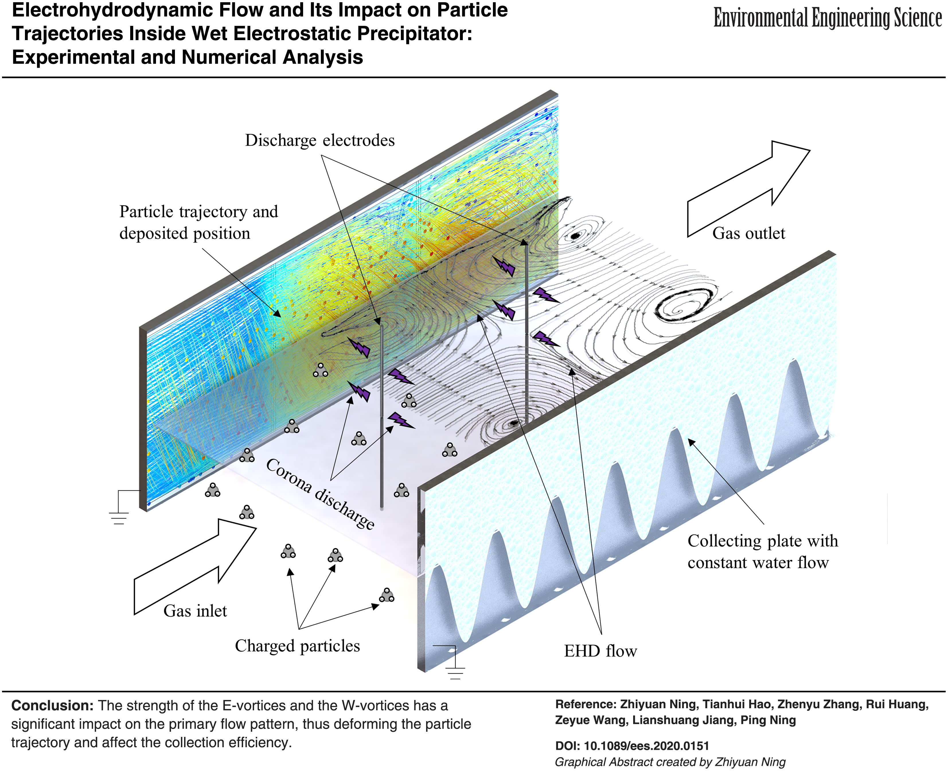
To analyze the flow pattern inside a typical wire-plate wet electrostatic precipitator (WESP) and its impact on particle trajectories, particle image velocimetry, and the finite element method were applied to visualize inner flow pattern. The flow pattern was primarily influenced by inner water flow along with the collector plates and the electrohydrodynamic (EHD) flow. Particle trajectories under various flow patterns were also studied. The results suggest that the EHD flow has a significant influence on the primary flow by creating vortex structures inside the WESP chamber. The water flow causes the inner flow pattern to become more complicated by generating vertical vortices. The particle trajectories were deformed with the inner flow patterns. Therefore, the collection efficiency can be severely hindered under various conditions. In this article, 16 different configurations were studied. The flow patterns of all configurations were given in two-dimensional images. Flow properties, that is, turbulent kinetic energy, turbulent dissipation rate, pressure, velocity magnitude and shear rate, and collection efficiency of each configuration are given in tabled data.

Introduction

Wet electrostatic precipitators (WESPs) are generally used as flue gas scrubbers to achieve ultra-low particulate matter emissions. The main difference between WESPs and ordinary electrostatic precipitators (ESPs) is the collecting plate cleaning process. WESPs remove deposited particles using a constant flow of liquid on the collecting plates, whereas ordinary ESPs shake particles off the collecting plates using a hammer. Therefore, WESPs do not exhibit emission spikes that are caused by the hammer cleaning strategy. However, the drawbacks of the cleaning strategy of WESPs is that the particle trajectories are less predictable, and the process produces waste sludge. Thus, further improvements are required to increase the collection efficiency to meet stricter emission standards. The first step toward this goal is to visualize the inner flow patterns, particle trajectories, and particle deposition patterns.

The power input of ESPs is correlated with collection efficiency. However, a higher power input generates a stronger electrohydrodynamic (EHD) flow caused by the corona discharge during operation. Recently, many researchers and industrial practitioners have proven that the generated EHD flow hinders the inner flow pattern and collection efficiency significantly (Ning et al., 2016a). This behavior is even more complicated for WESPs, which have more complicated inner flow patterns than ordinary ESP. Thus, a better understanding of particle movement under such complex conditions is required to improve WESP performance further.

To visualize the inner flow structure of WESPs, techniques such as laser Doppler velocimetry (Ims and Andreassen, 2002) and particle image velocimetry (PIV) (Kallio and Stock, 1990) are widely used. Podliński et al. (2011) thoroughly investigated the EHD flow inside various types of ordinary ESPs. Mizeraczyk (Chang et al., 2005) used two-dimensional (2D) and three-dimensional (3D) PIV to view the inner flow structure under the influence of the EHD flow. Their results indicated that the EHD flow influences the primary flow by creating vortex structures, causing the particle trajectories to become unpredictable and influencing the collection efficiency dramatically (Podliński et al., 2009).

However, experimental methods are usually limited by the restricted observation angles and conditions of ESPs, and the analysis of the inner flow patterns is difficult. Thus, numerical analysis has been widely used to complement flow visualization methods. Many numerical methods, such as the method of characteristics (Al-Hamouz, 2002), boundary element method (Zhao and Adamiak, 2008), computational structural mechanics (Elmoursi and Castle, 1987), discrete cell modeling (Levin and Hoburg, 1990), and finite difference method (Anagnostopoulos and Bergeles, 2002), have been developed. Soldati (2000) and Skodras et al., (2006) analyzed particle trajectories in multielectrode ESPs using a direct numerical simulation Lagrangian-driven method. The influence of the EHD flow on the dust collection efficiency was also compared. According to their result, the EHD flow significantly influences the collection efficiency and particle trajectories. Although different numerical analysis methods have been widely reported, each numerical method has its shortcomings for predicting flow structures due to the many assumptions and simplifications. Thus, experiments are still required, and a combination of flow visualization and simulations can be used to study the flow in WESPs.

During this work, a novel equipment was developed to observe the inner flow of WESP, and PIV method was applied to obtain actual flow distribution. The numerical analysis method was applied to obtain 3D flow structure, particle trajectory and deposited position on the collecting plates. Through those results, the deformation effect of EHD flow and water flow on the primary flow of WESP was revealed. The property of each configuration and related collection efficiency of different high-voltage (HV) electrode diameters were also given.

Materials and Methods

In this article, a cross-section of the inner flow structure of a WESP was investigated using the PIV method. The numeric analysis was used to investigate the 3D structures of the inner flow, electrostatic potential distribution, and particle collection efficiency.

PIV experimental setup

The quality of PIV images can be affected by many factors, especially the size of the observation area required for the cross-correlation algorithm (the fundamental PIV algorithm) (Wang et al., 2016). To obtain high-quality PIV results, a laboratory-scale transparent WESP was designed for flow pattern observation. The exploded view diagram and each component are shown in Fig. 1. The assembled WESP unit is shown in Fig. 2.

FIG. 1.

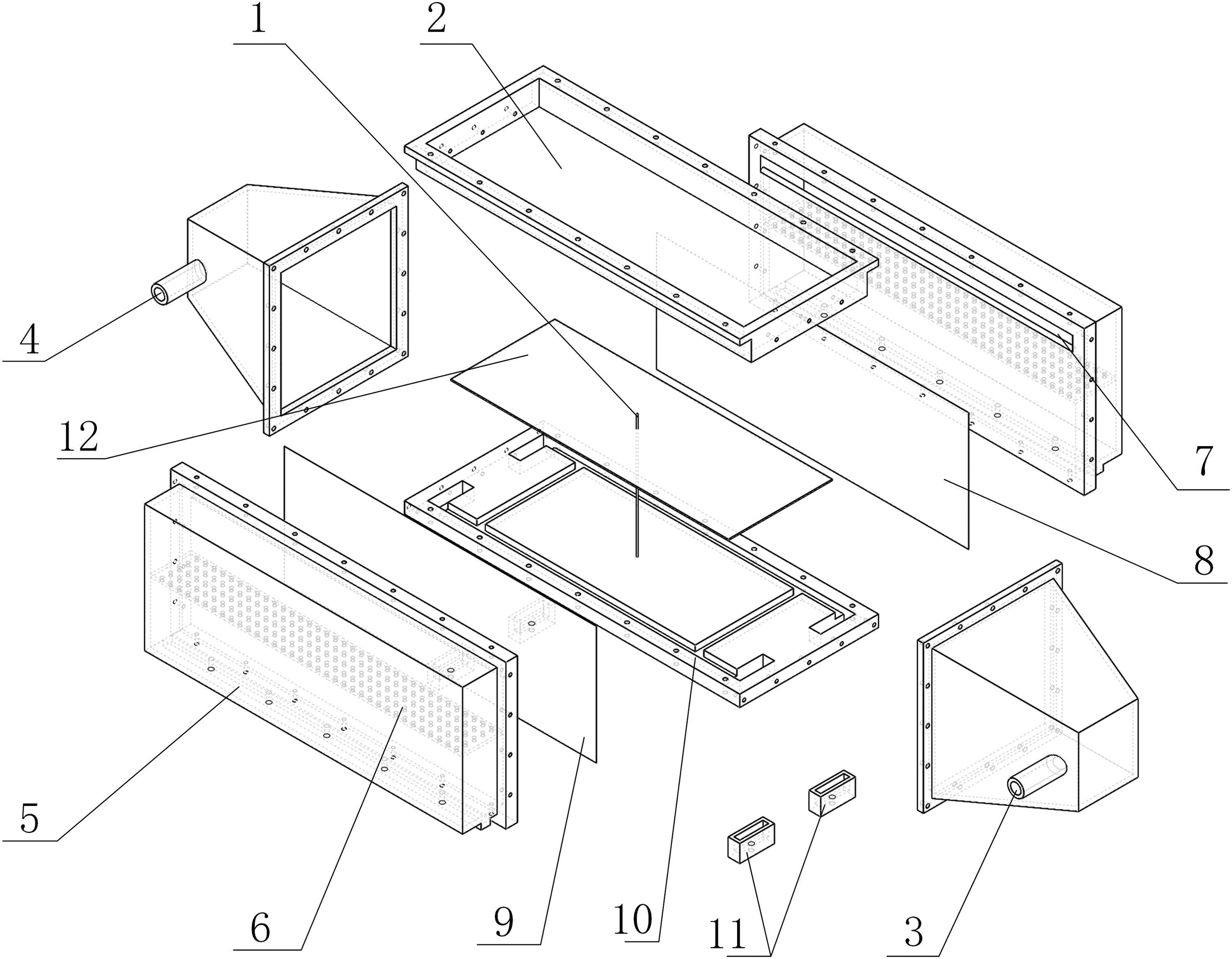
Exploded view of the laboratory-scale WESP designed for the PIV experiments. (1, HV electrode; 2, observation window/upper cover; 3, gas inlet; 4, gas outlet; 5, water inlet holes; 6, water tank; 7, pouring gate; 8 and 9, carbon fiber cloth; 10, drainage way/lower cover; 11, water outlet; 12, matte black mat). HV, high voltage; PIV, particle image velocimetry; WESP, wet electrostatic precipitator.

FIG. 2.

Schematic diagram of PIV experimental setup. (1, laser power supply; 2, synchronizer; 3, laser source; 4, optical lenses; 5, Fan; 6, Computer; 7, CCD camera; 8, WESP; 9, water pump; 10, water sink; 11, gas generator; and 12, HV DC power supply).

The outer wall of the WESP was made from acrylic. After assembling the unit, the upper and lower covers and two side water tanks formed a 200 × 200 × 600 mm³ wind tunnel. Flue gas was introduced to the tunnel through the flue gas inlet (3). After reaching the pouring gate (7), water formed a thin, uniformly distributed liquid film on the carbon fiber cloths (8 and 9), which also served as grounded collecting plates. The conductivity of carbon fiber is $0.3 \times 1 0^{6} S ∕ m$ . The EHD flow was being created by the corona discharge by a central electrode (1) connected to a HV source. The EHD flow traveled from the HV electrodes to the collecting plates (8 and 9). Thus, the directions of liquid film flow, flue gas flow, and EHD flow were perpendicular, and maximum interactions of the flows were achieved using this configuration, creating the best conditions for observing the inner flow pattern. Finally, using a matte-black mat as the background (12), high-quality PIV images were captured through the observation window (2).

During this experiment, a negative high-voltage DC power supply (peak output 60 kV/5 mA) was connected to the HV electrodes with two diameters (0.09 and 0.15 mm). Moxibustion smoke was used as tracer particles in this experiment due to its similar particle distribution and specific resistivity to coal power plant ashes (Shen et al., 2014); it also has excellent visibility to PIV camera. The number distribution of the tracer particle diameters can be seen in Fig. 3, which was measured using an electrical low-pressure impactor. The velocity of the inlet flue gas was set to 0.1 m/s, and the water flow rate was set to 0.2 m/s. The intensity of the EHD flow was adjusted by applying different voltages.

FIG. 3.

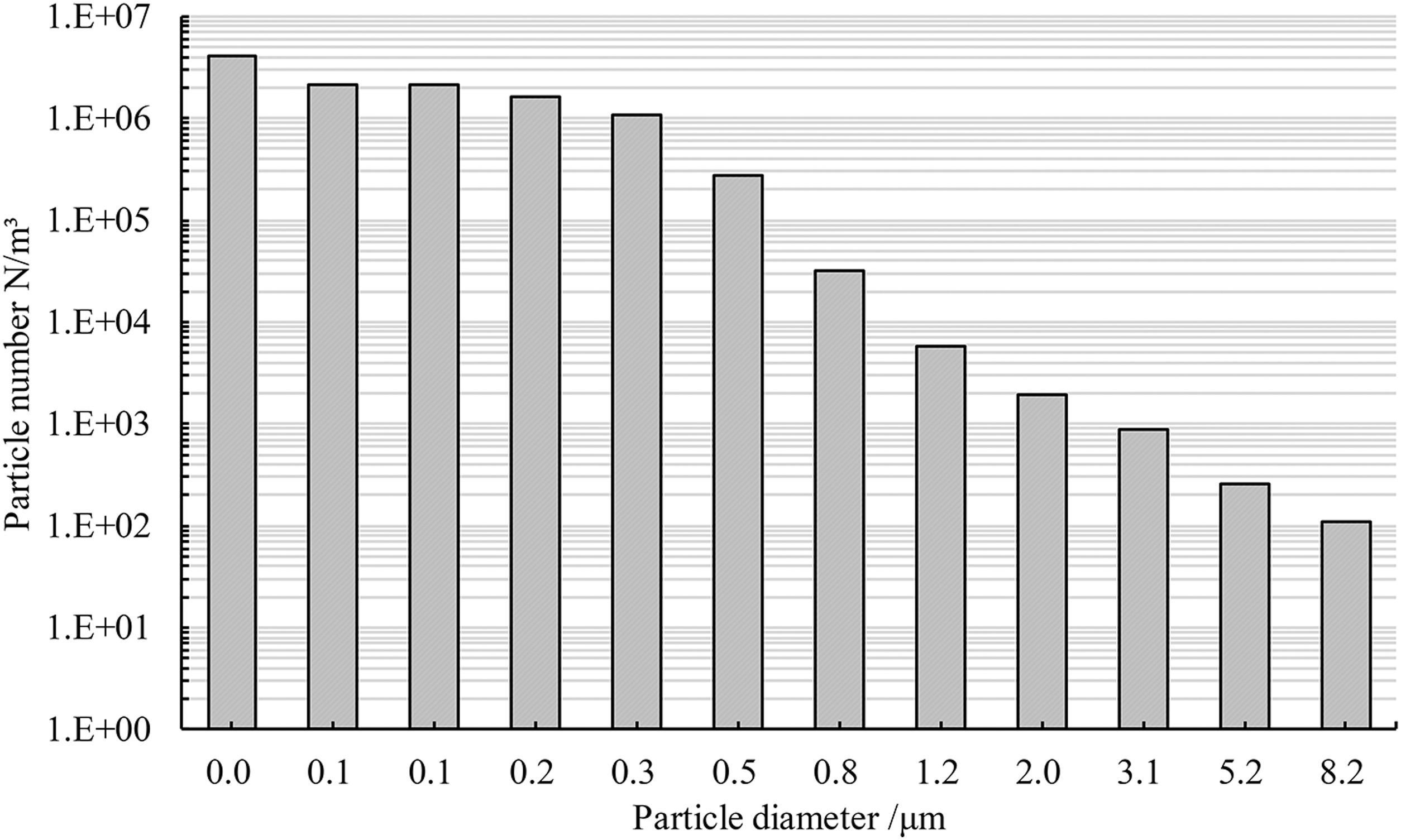
Number distribution of each particle diameter of chosen tracer particles.

Using a set of optical lenses, a second harmonic Nd:YAG laser source was transformed into a flat laser sheet, illuminating the observation section, which was located at the symmetric section of the WESP duct and perpendicular to the collecting plates and HV electrode. A laser-synchronized high-speed camera (7) captured 200 images with a 2,048 × 2,048 px² resolution for each experiment. The images acquired were processed by the two-image cross-correlation algorithm (Shi et al., 2015), yielding the flow structures. Time-averaged flow streamlines were calculated and are shown in Fig. 6.

FIG. 6.

Streamlines of the flow in the WESP for different electrodes and applied voltages.

Numerical analysis

To gain further insight into the flow patterns and compensate for the observation angle limitations of the PIV method, numerical analysis was applied. A 3D model with the same dimensions as the WESP used in the experiments but with shorter length due to PIV observation limitation was simulated. All the physical fields (gravity, gas flow, electric, and water flow) were coupled. Charged tracer particles were also released inside. Thus, this model could be used to determine the electric field and potential, particle charge, flow patterns, particle trajectories, and particle accumulation on the collecting plates.

This model was based on a typical line-plate WESP configuration: two grounded collecting plates were 0.2 m apart and located at each side of the WESP chamber (Y-Z plane). To simulate the water flow, these collecting plates moved with a prescribed downward (negative Z-axis direction) velocity of 0.2 m/s as additional boundary conditions, which could be turned on or off. Once HV wire electrodes (0.09- and 0.15-mm diameter, respectively) were located inside the center of the WESP chamber (the coordinates on the Y-axis were 0.15 m), primary gas flow was imposed into the WESP along the Y-axis direction as uniform laminar flow at various speeds. The parameters for these simulations are summarized in Table 1.

Table 1.

Major Parameters for Computational Fluid Dynamics Calculation Inside Wet Electrostatic Precipitator and Their Value

Parameters	d_g	l	t	M	ρ	k
Value	0.2 m	0.3 m	25°C	1.98 × 10⁻⁵ kg/(m·s)	0.746 kg/m³	2.4 × 10⁻⁴ m²/V
Description	Distance of ground plates	Length of WESP chamber	Flue gas temperature	Air viscosity	Air density	Ion mobility

WESP, wet electrostatic precipitator.

As shown in Fig. 4b, the completed mesh of flow chamber for calculation consists of 26,660 domain elements, 7,492 boundary elements, and 512 edge elements (10 boundary layers with 1.2 stretching factor). Several test simulation results suggested that when the boundary layer was greater than 7, no significant differences can be witnessed inside the boundary layer with increasing boundary layer number.

FIG. 4.

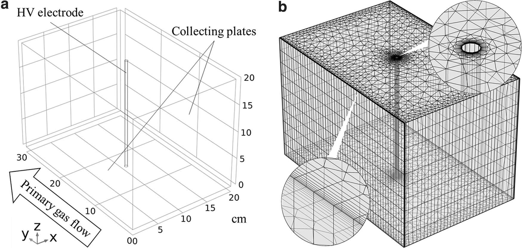
Three-dimensional model geometry and electrode configuration of WESP (a) configuration schematic (b) completed mesh of flow chamber for calculation.

The constitutive equations and related explanations for each physical field used for calculation are described in the following sections.

Electrostatic field constitutive equations

The relation between electric field E and potential V is defined by following the equation: $E = - \nabla V .$ (1)

The relation between the electric displacement vector D and electric field E is described as: $\begin{matrix} D = ε_{0} ε_{r} E \end{matrix} .$ (2)

Combining Eqs. (1) and (2), Gauss's law can be written as in the following form: $\begin{matrix} \nabla \cdot D = ρ_{v}, \end{matrix}$ (3) $\begin{matrix} \nabla \cdot ε_{0} ε_{r} E = ρ_{v} . \end{matrix}$ (4)

The boundary conditions for the ground electrodes were as follows: $\begin{matrix} n \cdot D = 0, \end{matrix}$ (5)

where∇ is the Hamiltonian operator, ρ_v is charge density, ɛ₀ is vacuum permittivity, ɛ_r is relative permittivity, n is the normal vector to the collecting plates. The boundary conditions for the above equations are:

charge conservation: the entire inner space of cabinet.

zero charge: all six sides of cabinet.

negative electric potential: the surface of the HV electrodes at 10 to 40 kV, respectively.

Particle charge equations

There are two particle charging mechanisms in an electrostatic field, depending on the particle size: diffusion charge and field charge. To simplify the calculation process during the simulations, only the field charge effect was considered, as the diffusion charge was negligible (Mizuno, 2000), the related particle charge equations are as follows (Wardman et al., 2014): $\begin{matrix} q (t) = q_{\infty} \frac{\frac{t}{τ}}{1 + \frac{t}{τ}}, \end{matrix}$ (6) $\begin{matrix} q_{\infty} = π ε_{0} \frac{3 ε_{s}}{ε_{s} + 2} d_{p}^{2} E, \end{matrix}$ (7)

\begin{matrix} τ = 4 \frac{ε_{0} E}{J}, \end{matrix}

(8)

where q_∞ is the saturated charge capacity of a particle, t is the time of charge, τ is field charge constant, d_p is the equivalent diameter of the particle, and J is the energy density.

Turbulent flow equations

The Reynolds-averaged Navier–Stokes (Wilcox and Ayyub, 2003) equations were used during the simulation to calculate the turbulent flow field. The gas was treated as a compressible Newtonian fluid, governed by the following equations:

Momentum conservation equation $\begin{matrix} ρ (u \cdot \nabla) u = \nabla \cdot [- p I + (μ + μ_{T}) (\nabla \cdot u) I - \frac{2}{3} ρ κ I] + F_{m f}, \end{matrix}$ (9)

Mass conservation equation $\begin{matrix} \nabla \cdot (ρ u) = 0, \end{matrix}$ (10)

Energy conservation equation $\begin{matrix} ρ (u \cdot \nabla) κ = \nabla \cdot [(μ + \frac{μ_{T}}{σ_{κ}}) \nabla κ] + P_{κ} - ρ ε, \end{matrix}$ (11)

Dissipation ratio $\begin{matrix} (u \cdot \nabla) κ = ρ (u \cdot \nabla) κ = \nabla \cdot [(μ + \frac{μ_{T}}{σ_{κ}}) \nabla κ] + C_{e 1} \frac{ε}{κ} P_{k} - C_{e 2} ρ \frac{ε^{2}}{k}, \end{matrix}$ (12)

\begin{matrix} ε = e p, \end{matrix}

(13)

\begin{matrix} μ_{T} = ρ C_{μ} \frac{k^{2}}{ε}, \end{matrix}

(14)

where u is the velocity field, p is the pressure, ρ is the density, I is the unitary matrix, F_mf is the main stream field vector, κ is the turbulent kinetic energy, ɛ is the vortex dissipation ratio, P_κ is the net output of dissipation of turbulent kinetic energy, μ is the viscosity coefficient of laminar flow, μ_T is viscosity coefficient of turbulent flow, and C and σ are correlation constants. The boundary condition for above equations are:

inlet: laminar uniform flow at various velocities (u_y = 0–0.2 m/s, u_x = u_z = 0 m/s)

outlet: pressure = 0 Pa

wall boundary condition (two side walls): set as moving wall (u_z = −0.2 m/s, u_x = u_y = 0 m/s). Top and bottom walls were set as stationary wall.

Momentum transfer to dispersed phase

An evenly dispersed particle in the flow field can experience several forces simultaneously, for example, drag, gravitational, Basset, and lift forces. Among these, the particle trajectories were mainly influenced by the drag force due to the turbulent flow inside the WESP.

The momentum transfer from the turbulent flow field to the particles in each grid node was calculated as follows: (Van Wachem et al., 2001; Enwald et al., 1996) $\begin{matrix} ρ_{a} ϕ_{a} [\frac{\partial}{\partial t} (u_{a}) + u_{a} \nabla \cdot (u_{a})] & = - ϕ_{a} \nabla p + \nabla \cdot (ϕ_{a} τ_{a}) \\ + ϕ_{a} ρ_{a} g + F_{m \cdot a} + ϕ_{a} F_{a}, \end{matrix}$ (16)

\begin{matrix} F_{d r a g, a} = - Ḟ_{d r a g, b} = β u_{s l i p}, \end{matrix}

(17)

\begin{matrix} u_{s l i p} = u_{b} - u_{a}, \end{matrix}

(18)

where g is the gravitational acceleration vector, Φ is particle diameter, F_drag is the drag force, U_slip is relative sliding velocity, F_m is the momentum transfer between phases, F denotes other volume forces, and subscripts a and b refer to the two phases (the particles and gas flow). the boundary condition for above equations are:

wall condition for all surfaces, except inlet and outlet: particle freeze when contact.

Particle charge number: obtained by Eqs. (6)–(8)

Drag force: stokes law, velocity dynamic viscosity, and density were all from the turbulent flow result.

Electric force: from electrostatics result.

Coupling methods

The calculation contains three steps: first, by using the plasma module to acquire electric potential and electric field results. Second, the data obtained from the first step were used as an initial value on the turbulence flow module to acquire flow distribution result. Finally, the velocity map $\nabla u^{T}$ (acquired by step 2) was used as an initial value on the particle tracing module to acquire particle migration result. Due to particle number are far less than the real ESP, and only fine particle was considered (particle number and size must be large enough to create visible influence on primary flow), the influence of particle motion on airflow can be neglected. Thus, this simulation was a one-way coupling.

The simulation was first calculated as the steady turbulence flow due to the flow inside WESP is time irrelevant when the primary flow and flow cabinet was fixed. Thus, the $\frac{\partial}{\partial t}$ from k-ɛ equation was neglected during turbulence flow calculation (step 2). However, the momentum transfer from the fluid to the particle is time dependent due to the particle position constantly changing. Thus, the momentum transfer equation (step 3) needs considering $\frac{\partial}{\partial t}$ to acquire particle position at various time.

Results and Discussion

PIV results

Electrical characteristics of WESP

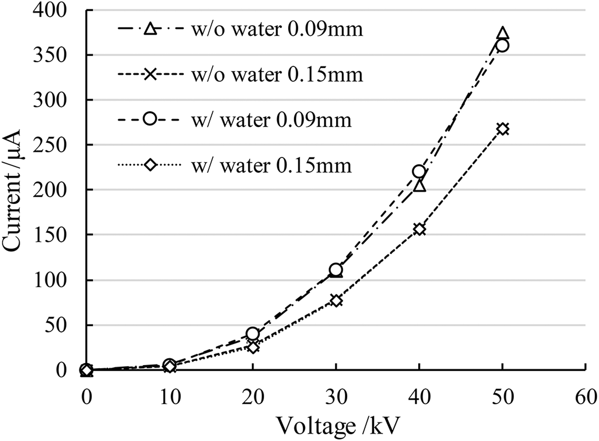
The electrical characteristics of the laboratory-scale WESP under various configurations were measured first. HV electrodes with two different diameters were installed. The ambient temperature was 20°C, and the relative humidity was 95% under conditions with water flow (hereafter refers as w/water) and 40% without water flow (hereafter refers as w/o water). The I-V curves for each configuration are shown in Fig. 5

FIG. 5.

Electrical characteristics of WESP under various configurations.

Water flow inside the WESP had little effect on the overall electrical characteristics. The difference between the I-V curves primarily depended on the diameter of the electrodes, that is, the discharge intensity increased only with increased electrode curvature, with or without water flow. All the configurations generated corona discharges at around 5 kV. The corona discharge current of the 0.09 mm electrode increased more rapidly compared with the 0.15 mm electrode. The stronger discharge current also indicates that stronger EHD flow was generated.

Flow patterns

Figure 6 is the flow pattern result shown as 2D plane images, the location of this plane was in the middle of the WESP cabinet, as shown in Fig. 2 (the green plane indicates the illuminated area of the cabinet by laser sheet and the observation area). The camera was positioned at the top of the WESP cabinet; thus, Fig. 6 shows a top view of the general flow pattern.

As shown in Fig. 6, the flow fields in all configurations were symmetric overall. This was due to the centrally located HV electrodes discharging to both collecting plates with equal intensity, and thus, identical EHD flow was generated to both collecting plates.

For the 10 kV condition, particles were not significantly dispersed by the corona discharge because there was almost no EHD flow created at this low voltage. Thus, for the 0.15 mm electrode w/o water (line 1, column 1), particles were only driven by electric field force, showing unidirectional motion toward the collecting plates. Therefore, the primary flow remained laminar and slightly bent toward the collecting plate after passing the HV electrode. However, w/water (line 2, column 1), another drag force was created due to the vortices generated by water movement (hereafter referred to as W-vortices, which can be seen clearly in Fig. 9), dragging particles toward the collecting plates.

FIG. 9.

Streamline of inner flow of WESP under various applied voltages and primary flow speed (side view).

The phenomenon can also be observed for the 0.09 mm electrode configuration (line 3, column 1). However, due to the increased electrode curvature, the discharge strength also increased, and the EHD flow developed and formed vortices (hereafter refers as E-vortices) before the HV electrode. These vortices compressed the primary flow, leading pressure changes along the wind tunnel. In response to the vacuum generated downstream by the vortices, a backflow also formed near the outlet. Similarly, under the w/water configuration (line 4, column 1), the diameters of the vortices decreased compared with the previous configuration. This occurred because the flow pattern was diverted by the W-vortices, creating a 3D flow instead of the 2D flow that formed in the previous configuration.

A similar phenomenon occurred for the 0.15 mm configuration with a potential of 20 kV. Two obvious symmetrical E-vortices and two back-flow-induced vortices were generated simultaneously in the w/o water configuration (line 1, column 2). However, the vortices dispersed as soon as water flow began (line2, column 2). This suggests that E-vortices and W-vortices had equal strengths. For the 0.09 mm electrode configuration (line 4, column 2), the strengths of the E-vortices exceeded those of the W-vortices, resulting in the compression of the vortices, but not their dispersal. The same phenomenon occurred with 30 and 40 kV potentials (columns 3 and 4). Under these conditions, the W-vortices were no longer the main factor influencing the shape of the flow field because stronger E-vortices were created by the rapidly increased discharge.

Due to PIV limitations, only a cross-section of the air tunnel could be observed, and only a 2D flow field could be obtained. Thus, the influence of water flow on the entire flow field could only be estimated by the shapes of the vortices, which is not an accurate method. To overcome this limitation, 3D numerical analysis was used (Yamamoto and Velkoff, 2006).

Numerical analysis

Electric field distributions and their impact on particle charge efficiency

Based on the geometry and conditions discussed in the Numerical Analysis section. The electric field and electric potential were first calculated. It can be seen from Fig. 7 that the isopotential lines were uniformly distributed along the HV electrodes. The isopotential lines formed circles near the HV electrodes and ellipses near the collecting plates.

FIG. 7.

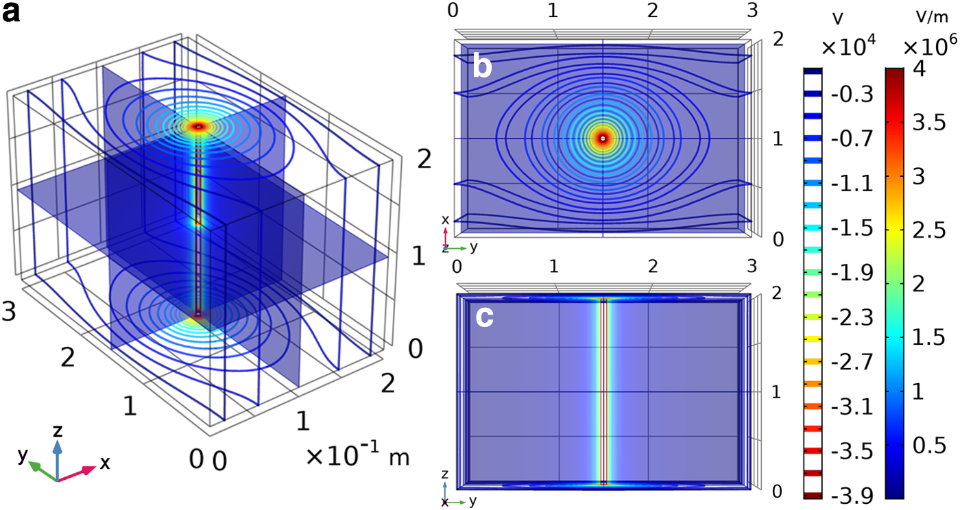
Schematic diagram of electric field distribution (multislice plot, right legend) and electric potential distribution (contour plot, left legend) for an applied voltage of 40 kV (a) isometric view (b) top view (c) side view.

As shown in the multislice plot in Fig. 7, the area with a high electric field intensity (where corona discharge occurs) vanishes rapidly with the distance to the HV electrodes. In this region, particles have the maximum charge efficiency, and the Coulomb force was the strongest. However, the electric field intensity, particle charge efficiency, and particle trajectory decreased rapidly in the other regions.

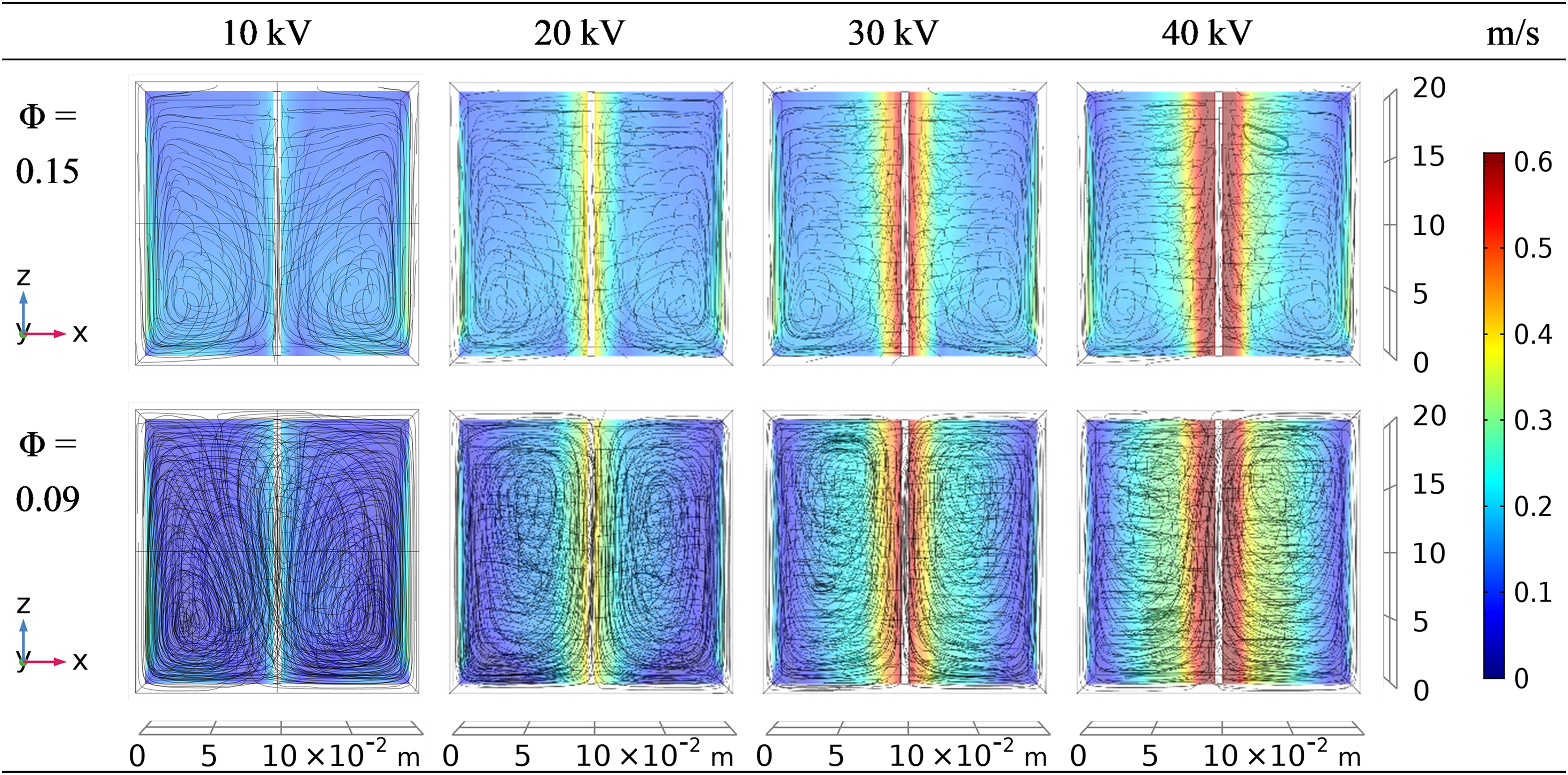
Figure 8 shows the velocity fields and streamlines for different voltages under the w/and w/o water conditions. The simulation results agreed with the PIV results. The 3D numerical model allows the flow field to be analyzed in any direction.

FIG. 8.

Velocity field and streamlines for applied voltages of 20 kV (left two columns) and 40 kV (right two columns) with various primary flow speeds.

Flow field and streamlines

The flow structures under the w/o water condition were similar to the PIV results. Form Fig. 8, the diameter of the electrode can make a significant impact on generated E-vortices. When only 10 kV voltage applied (first column), the primary flow has been distorted as a different variation. When 0.15 mm HV electrode was installed, generated E-vortices only created distortion slightly at the downstream of the electrode. However, when 0.09 mm electrode was installed, generated E-vortices has already occupied the entire flow chamber. but the strengths of E-vortices were weak at this power input. Under w/water configuration (column 1, line 4), the E-vortices has soon been overcome, and the W-vortices has dominated the entire chamber.

As the input voltage increased to 20 kV, the E-vortices has expanded and created a certain level of low pressure and backflow area located downstream of the electrode for 0.15 mm configuration (column 2, line 1 and 2). Furthermore, it was noteworthy that for the 0.09 mm w/water configuration (column 2, line 4), despite the distortion of W-vortices persists, the shape of E-vortices were partially recognizable, meaning that the deformation amplitude of both vortices to primary flow was similar at this point. This phenomenon can be interpreted as both forces having the same strengths and contributing equally to the general flow field deformation.

Along with increasing input voltage, the E-vortices continue producing more significant low pressure and backflow regain at the back of the electrode for 0.15 mm configuration (line 1, column 3 and 4). However, the near unaffected upstream flow pattern suggesting that the strength of E-vortices created by the thicker electrode was unmatched than the thinner electrode.

For 30 kV and above, the flow pattern of 0.09 mm electrode configuration under w/o water condition (line 3, column 3 and 4) has clearly shown a 3D pattern, meaning that the strength of E-vortices is already high enough to create enough shear forces between different layers in the X-Y plane, causing momentum transfer to occur along Z-axis, giving the general flow pattern a 3D appearance. It should be noticed that due to the roughness and imperfection of the electrode installed in the actuate ESP, this momentum transfer along the Z-axis will occur at a much lower applied voltage.

In high-input voltages and w/water conditions (line 4, column 3 and 4), E-vortices regained domination of entire flow pattern, generating four vortex structures. Those vortices will create a vacuum region. Particles trapped inside will cost a much longer time doing continuous spiral movement instead of being driven to the collecting plates rapidly, despite the significant charge efficiency and driving forces under those operating conditions, greatly hindering the collection efficiency. Thus, those vortex structures must be prevented or minimized. Based on the simulation result, the increasing voltage does not always result in better collection efficiency, especially for fine particles. A proper diameter of the electrode with a lower applied voltage can prevent the generation of vortex structures, resulting in higher collection efficiency.

In summary, higher input voltage increases the particle charge efficiency and provides larger Coulomb forces, but results in severe EHD flow, leading to a chaotic flow distribution and lower collection efficiency. To minimize the influence of the vortex structures on the collection efficiency, the primary flow velocity, applied voltage, and water flow speed needs to be carefully balanced. For example, larger particles will be less affected by the flow pattern due to the higher charge ratio, and thus, a higher applied voltage and water flow speed can be used. However, fine particles, especially with diameters less than 1 μm can be easily influenced by the inner flow pattern. Thus, a properly applied voltage and water flow speed are critical to increasing collection efficiency.

Figure 9 shows the streamlines of the side view (X-Z plane) for various voltages and primary flow velocity. This is an ideal angle to intuitively observe the impact of water flow on the general flow field because the water flow direction (pointing along Z-axis) and EHD flow direction (pointing along X-axis) are perpendiculars. We can see the W-vortices were dominant in the entire section when a low voltage was applied (fewer E-vortices generated). However, when a higher voltage was applied, along with the gradual appearance of E-vortices, streamlines became cluttered. As the EHD flow increases, the strength of the W-vortices was gradually overwhelmed, creating mixed vortices.

Overall, the influence of the water flow on the general flow field was greater than the EHD flow. From Fig. 9, the vertical vortices persisted regardless of the EHD flow. When the primary flow velocity increased, the decrease in amplitude of the W-vortices was smaller compared with the E-vortices.

In conclusion, the water flow inside WESP creates a 3D internal flow structure, and the particle trajectories will be more complicated than those in a typical ESP.

Particle trajectories

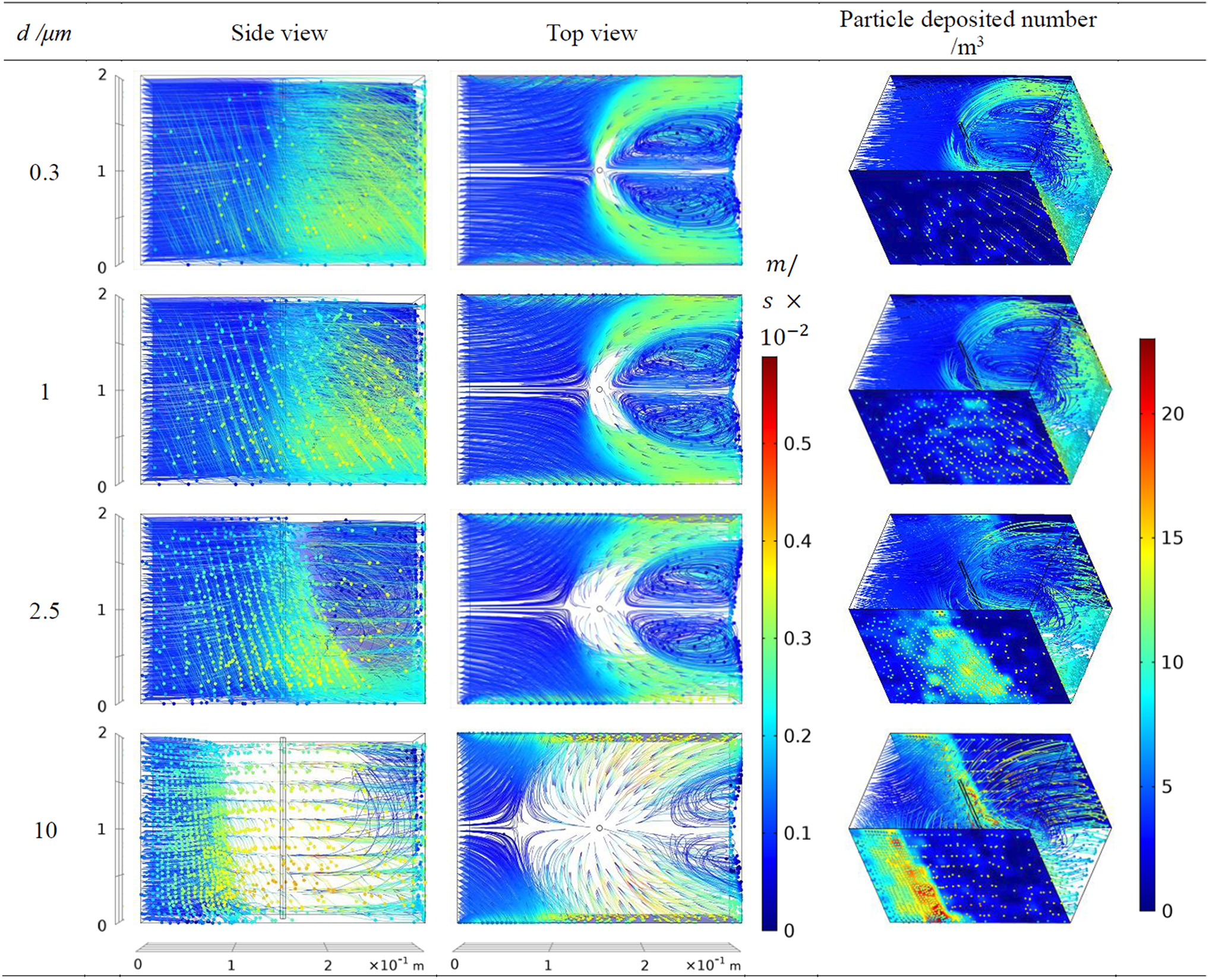
To investigate the particle trajectories, 4,000 tracing particles with four diameters (0.3, 1, 2.5, 10 μm) were released into the WESP chamber, and their trajectories were determined. The particles were evenly distributed and released simultaneously at the inlet, which guaranteed that all particles had the same momentum when entering the chamber. To maximize the influence of all the factors on the particle trajectories, the voltage was set to 40 kV with 0.15 mm diameter HV electrode, and the primary flow rate was set to 0.1 m/s. The particles deposited upon contact with the collecting plates (zero bounce rate).

Figure 10 shows the particle trajectory from the side and top views, and the particle deposition locations for the different diameters are also shown. The accumulation of particles was calculated with the following equation:

FIG. 10.

Particle trajectories for various particle diameters and deposited positions.

\begin{matrix} R_{A c c u m u l a t i o n} = \sum_{p = 1}^{N_{p a r i c l e s}} \frac{q_{m}}{A_{f a c e}} [k g ∕ m^{2} s] \end{matrix}

(19)

where q_m is the mass flow rate of particles and A_face is the grid area of collecting plates.

Furthermore, as shown in the particle charge Eq. (5), the particle charge is proportional to the diameter, indicating that 10 μm particles will withstand the strongest Coulomb forces (several orders of magnitude stronger than other particles). The 10 μm particles were almost completely deposited on the collecting plates even before reaching the first electrode. With water flow, the particles located at the bottom of the WESP tended to move farther forward than the particles at the top. This occurred because the W-vortices carried some of the particles back to the center of the wind tunnel before they reached the collecting plates. Thus, the bottom particles traveled farther inside the WESP than the top ones.

As the particle diameters decreased, the quantity of charged particles decreased sharply, because the influence of the Coulomb force on the particle trajectory also decreased. This allowed particles to withstand greater drag forces, and the particle trajectories more closely followed the flow field as the diameters decreased. As shown in Fig. 10, the trajectory of the 0.3 μm particles nearly overlapped the streamlines shown in Fig. 8. This can explain the low collection efficiency of many ordinary ESPs for particles smaller than 1 μm. Smaller particles not only experience weaker Coulomb forces, but also become trapped in the vortex zone, making it difficult for them to reach the collection plates. Furthermore, as shown in Fig. 10, particles have higher velocities when they are near the collecting plates. The electric field force was also weaker in this region. The combination of these phenomena reduced the overall particle residence times and lowered the collection efficiency. Figure 10 also indicates that the deposition area moved further downstream and eventually blurred as the particle diameter decreased, indicating that most particles left the WESP chamber before they could impact the collecting plates.

Effect of water flow on dust collection efficiency

The effects of water flow on the collection efficiency at a flow velocity of 0.1 m/s and voltage in 30 kV with 0.09 mm diameter HV electrode were calculated and are compared in Table 2, where d is the particle diameter, N_d is the number of captured particles, N_e is the number of escaped particles, and η is the collection efficiency.

Table 2.

Collection Efficiency of Particles of Different Diameters with a Primary Flow Speed of 0.1 m/s

d/μm	N_d		N_e		η%
d/μm	w/o water	w/water	w/o water	w/water	w/o water	w/water
10	2,550	2,557	1,450	1,443	63.8	63.9
2.5	1,645	1,824	2,355	2,176	41.1	45.6
1	1,060	1,106	2,940	2,894	26.5	27.7
0.3	509	528	3,491	3,472	12.7	13.2

The collection efficiency was significantly influenced by the water flow. Generally, the collection efficiencies under the w/water condition were higher than those obtained under the w/o water condition. The difference was as large as 10% for 2.5 μm particles. However, the difference decreased as the particle size decreased because the number of escaped particles was sufficiently large, and the water flow had little influence on the collection efficiency. As mentioned previously, particles in this size range followed the streamlines to the outlet despite the chaotic flow structure because they had limited charges.

Other flow property results and collection efficiency results are shown in Table 3. Each shown number represents the volume average of the entire calculation area of each flow property under various configurations. Last 4 columns show related collection efficiency of each size of particles.

Table 3.

Flow Property Results and Collection Efficiency Results Under All Simulated Configurations

Configuration			Flow property					Collection efficiency
Electrode diameter	Voltage	Wall speed	Turbulent kinetic energy	Shear rate	Turbulent dissipation rate	Pressure	Velocity magnitude	0.3 μm	1 μm	2.5 μm	10 μm
(mm)	(kV)	(m/s)	(m²/s²)	(1/s)	(m²/s³)	(Pa)	(m/s)	(η%)	(η%)	(η%)	(η%)
0.15	10	0	7.71⁻⁴	2.28	1.62⁻³	2.66⁻⁴	4.94⁻²	59.9	61.8	64.6	73.2
	10	1	2.19⁻³	5.04	7.22⁻³	2.38⁻⁴	7.98⁻²	66.5	71.3	72.2	74.1
	20	0	5.99⁻⁴	2.28	1.71⁻³	4.66⁻³	1.05⁻¹	19	33.3	48.5	65.6
	20	1	1.81⁻³	4.75	6.65⁻³	5.81⁻³	1.24⁻¹	20.9	39	51.3	66.5
	30	0	6.56⁻⁴	2.57	2.01⁻³	6.75⁻³	1.43⁻¹	10.5	23.8	40.9	64.6
	30	1	1.81⁻³	4.85	6.75⁻³	8.08⁻³	1.62⁻¹	10.5	24.7	45.6	64.6
	40	0	8.36⁻⁴	2.66	2.47⁻³	8.86⁻³	1.91⁻¹	5.6	17.1	36.1	63.7
	40	1	1.91⁻³	4.94	7.22⁻³	1.05⁻²	2.01⁻¹	7.3	18.1	40.9	63.7
0.09	10	0	1.14⁻³	3.52	3.33⁻³	4.85⁻⁴	7.79⁻²	58	60.8	64.6	71.3
	10	1	2.28⁻³	5.8	8.86⁻³	9.95⁻⁴	9.51⁻²	61.8	70.3	72.2	73.2
	20	0	1.05⁻³	3.23	3.61⁻³	8.08⁻³	1.24⁻¹	18.1	33.3	47.5	64.6
	20	1	2.01⁻³	5.61	8.17⁻³	9.52⁻³	1.33⁻¹	19	41.8	49.4	65.6
	30	0	1.05⁻³	3.52	3.99⁻³	1.05⁻²	1.62⁻¹	12.7	26.5	41.1	63.8
	30	1	2.09⁻³	5.7	8.86⁻³	1.24⁻²	1.71⁻¹	13.2	27.7	45.6	63.9
	40	0	1.24⁻³	3.71	4.56⁻³	1.33⁻²	2.01⁻¹	8.6	20	37.1	61.8
	40	1	2.19⁻³	5.8	8.86⁻³	1.52⁻²	2.09⁻¹	9.5	20	41.8	61.8

In actual WESPs, fine particles easily agglomerate with water vapor, forming larger diameter particles. Therefore, the WESP would be more efficient at capturing fine particles in practical operations. Also, during actual industrial operations, there are more factors that can affect the collection efficiency that were not considered in the simulations, which require further studies.

Conclusion

The flow field in a laboratory-size WESP was analyzed using PIV and finite element multiphysical field coupling methods. The main purpose of this study was to visualize the flow field inside WESP, which has been rarely reported and is usually difficult to acquire. The trajectories of charged particles under the influence of an electric field and flow field were evaluated. The result suggests that the flow field in the WESP becomes rather complicated in the presence of water flow along with the collecting plates and EHD flow, and the inner flow pattern affects the collection efficiency.

The PIV results indicate that, under certain conditions (0.15 mm HV electrode, 20 kV applied voltage, 0.1 m/s primary flow, and 0.2 m/s water flow), the strength of the EHD flow forms vertical vortices. According to the simulation, E-vortices and W-vortices with equal strengths were formed under the 20 kV with 0.15 mm diameter HV electrode configuration, which agreed with the PIV result. The three major parameters (applied voltage, water flow speed, and primary flow velocity) must be chosen properly. Otherwise, a chaotic inner flow pattern and poor collection efficiency will result. Furthermore, the collection efficiency was highly dependent on particle diameter, and particles with 2.5 μm diameters were most affected by the inner flow pattern.

There are other ways to extend this work to further enhance the applicability of this model, such as adding more complex physics, which includes matter transfer and temperature transfer between liquid and gas phases, various HV electrodes, and shape of the collecting plates. Furthermore, 3D PIV results are favorable when comparing and adjusting simulation results.

Flow field visualization and particle trajectory analysis not only indicated the particle motion trends but also identified the main factors that hinder the collection efficiency. Further improvements to the collection efficiency by flow field modifications can be made (Ning et al., 2016b) only if the flow field characteristics are fully understood. Thus, flow field visualization is critical for future WESP design and optimization.

Footnotes

Acknowledgment

The authors thank LetPub for its linguistic assistance during the preparation of this article.

Author Disclosure Statement

No competing financial interests exist.

Funding Information

This study was funded by the Yunnan Provincial Science and Technology Department's Science and Technology program (2018FD013) and National Demonstration Center for Experimental Chemistry and Chemical Engineering Education (Yunnan University).

References

Al-Hamouz

Z.M.

(2002). A combined algorithm based on finite elements and a modified method of characteristics for the analysis of the corona in wire-duct electrostatic precipitators. IEEE Trans. Ind. Appl. 38, 43.

Anagnostopoulos

, and Bergeles

(2002). Corona discharge simulation in wire-duct electrostatic precipitator. J. Electrostat. 54, 129.

Chang

J.S.

, Dekowski

, Podlinski

, Brocilo

, Urashima

, and Mizeraczyk

(2005). Electrohydrodynamic gas flow regime map in a wire-plate electrostatic precipitator under positive coronas. In: CEIDP’05. 2005 Annual Report Conference on Electrical Insulation and Dielectric Phenomena. IEEE, Nashville, TN,, 2005, 461.

Elmoursi

A.A.

, and Castle

G.S.P.

(1987). Modeling of corona characteristics in a wire-duct precipitator using the charge simulation technique. IEEE Trans. Ind. Appl. IA-23, 95.

Enwald

, Peirano

, and Almstedt

A.-E.

(1996). Eulerian two-phase flow theory applied to fluidization. Int. J. Multiphase Flow. 22, 21.

Ims

R.A.

, and Andreassen

H.P.

(2002). On the modelling of the electro-hydrodynamic flow field in electrostatic precipitators. Flow Turbul. Combust. 68, 63.

Kallio

G.A.

, and Stock

D.E.

(1990). Flow visualization inside a wire-plate electrostatic precipitator. IEEE Trans. Ind. Appl. 26, 503.

Levin

P.L.

, and Hoburg

J.F.

(1990). Donor cell-finite element descriptions of wire-duct precipitator fields, charges, and efficiencies. IEEE Trans. Ind. Appl. 26, 662.

Mizuno

(2000). Electrostatic precipitation. IEEE Trans. Dielectr. Electr. Insul. 7, 615.

10.

Ning

, Cheng

, Shen

, Li

, and Yan

(2016a). Electrode configurations inside an electrostatic precipitator and their impact on collection efficiency and flow pattern. Eur. Phys. J. D. 70, 126.

11.

Ning

, Podlinski

, Shen

, Li

, Wang

, Han

, and Yan

(2016b). Electrode geometry optimization in wire-plate electrostatic precipitator and its impact on collection efficiency. J. Electrostatics. 80, 76.

12.

Podliński

, Niewulis

, and Mizeraczyk

(2009). Electrohydrodynamic flow and particle collection efficiency of a spike-plate type electrostatic precipitator. J. Electrostatics. 67, 99.

13.

Podliński

, Niewulis

, Shapoval

, and Mizeraczyk

(2011). Electrohydrodynamic secondary flow and particle collection efficiency in a one-sided spike-plate type electrostatic precipitator. IEEE Trans. Dielectr. Electr. Insul. 18, 1401.

14.

Shen

, Zheng

, Ning

, Wang

, Han

, and Yan

(2014). PM 10 and PM 2.5 Emission control by electrostatic precipitator (ESP) for coal-fired power plants IV: Investigations on electrostatic precipitation by means of 2D PIV technique. Sci. Technol. Rev. 32, 43.

15.

Shi

, Wei

, and Pang

(2015). A modified cross-correlation algorithm for PIV image processing of particle-fluid two-phase flow. Flow Meas. Instrum. 45, 105.

16.

Skodras

, Kaldis

S.P.

, Sofialidis

, Faltsi

, Grammelis

, and Sakellaropoulos

G.P.

(2006). Particulate removal via electrostatic precipitators—CFD simulation. Fuel Process. Technol. 87, 623.

17.

Soldati

(2000). On the effects of electrohydrodynamic flows and turbulence on aerosol transport and collection in wire-plate electrostatic precipitators. J. Aerosol Sci. 31, 293.

18.

Van Wachem

B.G.M.

, Van der Schaaf

, Schouten

J.C.

, Krishna

, and Van den Bleek

C.M.

(2001). Experimental validation of Lagrangian-Eulerian simulations of fluidized beds. Powder Technol. 116, 155.

19.

Wang

, Xie

, Xu

, Li

, and Zhou

(2016). Experimental study on EHD flow transition in a small scale wire-plate ESP. Meas. Sci. Rev. 16, 134.

20.

Wardman

, Wilson

, Hardie

, and Bodger

(2014). Influence of volcanic ash contamination on the flashover voltage of HVAC outdoor suspension insulators. IEEE Trans. Dielectr. Electr. Insul. 21, 1189.

21.

Wilcox

R.C.

, and Ayyub

B.M.

(2003). Uncertainty modeling of data and uncertainty propagation for risk studies. In: 4th International Symposium on Uncertainty Modeling and Analysis, ISUMA 2003, IEEE, College Park, MD, 184.

22.

Yamamoto

, and Velkoff

H.R.

(2006). Electrohydrodynamics in an electrostatic precipitator. J. Fluid Mech. 108, 1.

23.

Zhao

, and Adamiak

(2008). Numerical simulation of the electrohydrodynamic flow in a single wire-plate electrostatic precipitator. IEEE Trans. Ind. Appl. 44, 683.