
Abstract
We apply Cattaneo's relaxation approach to the one-dimensional coupled Boussinesq groundwater flow and advection-diffusion-reaction equations, commonly used in engineering applications to simulate contaminant transport in the subsurface. The diffusion-type governing equations are reformulated as a hyperbolic system, augmented by an equation that can be interpreted as a momentum balance. The hyperbolization enables an efficient unified computation of the primary variable and its gradients, for example piezometric head and unit discharge in the Boussinesq equation. An augmented Roe scheme is used to solve the hyperbolic system. The hyperbolized system of equations is studied in a set of steady state and transient test cases with idealized geometry. These test cases confirm the equivalence of the hyperbolic system to its original formulation. The larger time step size of the hyperbolic equation is verified theoretically by means of a stability analysis and numerically in the test cases. Finally, a reach-scale application of flow and transport across a river meander is considered. This application case shows that the performance of the hyperbolic relaxation approach holds for more realistic groundwater flow and transport problems, relevant to water resources management.
Introduction
Reactive transport models (RTMs) are widely used to investigate coupled physical and biogeochemical processes in natural and engineered systems (Steefel et al., 2015). Mechanistic insights gained with RTMs have broad relevance for water, energy, and the environment with applicability from the critical zone to the deep subsurface (Clarens and Peters, 2016; Li et al., 2017). The RTM simulations are underpinned by the numerical solution of a set of mixed differential and algebraic equations that often have significant computational costs (Steefel et al., 2015).
The differential equations that describe groundwater flow and solute transport that are part of RTMs usually include parabolic terms. Examples of these types of equations are the Boussinesq groundwater flow equation (BE) and the advection-diffusion-reaction equation (ADR). The BE is a nonlinear parabolic partial differential equation (PDE), and the ADR is a mixed-type parabolic-hyperbolic PDE. The parabolic nature of these equations poses two challenges. First, the time step size of the BE is constrained by a parabolic constraint of O(h2) (Toro and Montecinos, 2014). Second, the unit discharge in the BE is not a primary conserved variable, but instead is computed from the gradient of the piezometric head. Thus, the piezometric head and the unit discharge are not necessarily computed with uniform accuracy (Nishikawa, 2007). The same challenges apply to the parabolic part of the ADR. Reformulating the equations in hyperbolic form makes it possible to overcome these issues that hamper efficient simulation (Nishikawa, 2007; Toro and Montecinos, 2014).
In this work, we apply a relaxation approach to convert the BE and ADR into a first-order hyperbolic system with the objective of enabling efficient simulations. The BE and single-component ADR are used here as examples of the general groundwater flow and reactive transport equations but also because they are commonly used in water resources management (Boyraz and Kazezyılmaz, 2018). They also make it possible to simplify simulations of unconfined systems dominated by horizontal processes when the Dupuit assumptions hold (Bear, 1972). To model contaminant spreading—or the transport of any arbitrary chemical species—in the subsurface, the BE can be coupled with the ADR.
The relaxation approach employed in this work was developed in Nishikawa (2007) to obtain steady-state solutions for a diffusion equation using a residual distribution approach, and it is extended to the Navier-Stokes equations (Nishikawa, 2011). Transient solutions have been proposed for advection-diffusion equations in Mazaheri and Nishikawa (2014), and more recently for the heat equation in He and Roe (2019). However, the relaxation approach has not yet been applied to groundwater flow and reactive transport problems. The specific relaxation approach used in these publications is Cattaneo's relaxation approach (Cattaneo, 1958)—see Toro and Montecinos (2014) for a discussion of the advantage of this particular relaxation approach over other existing ones. In the literature, Cattaneo's relaxation approach is considered as a solely numerical treatment that hyperbolizes diffusion-type equations. More generally, for example in Jin and Xin (1995) and Jin et al. (1998), relaxation approaches enforce the hydrodynamic limit to kinetic models of the Boltzmann equation through diffusive rescaling. However, this interpretation is not valid for Cattaneo's relaxation. Following the discussion in LeVeque (2002), we consider the relaxation system to be an equilibrium system that is subject to perturbations. The equilibrium state of this system is the original diffusion-type equation. The hyperbolization can then be considered as a (small) perturbation around this equilibrium state that allows to solve the system more efficiently. The system relaxes to its equilibrium state, that is converges toward the diffusion-type equation, fast enough, such that the perturbation has a negligible effect on the model solution.
When applied to the BE and ADR, the resulting first-order hyperbolic equations (hereinafter referred to as hBE and hADR, respectively) may be written with the unit discharge as a primary variable. Thus, it may be computed simultaneously with the piezometric head or the species concentration and with uniform accuracy. The time step size limitation is formally relaxed to O(h), although, as shown in Nishikawa (2010), the parabolic constraint of O(h2) is implicitly contained in the Courant–Friedrichs–Lewy (CFL) condition of the hyperbolic system (Courant et al., 1928).
In what follows, we derive the hBE and hADR and discuss some of their properties. We present an augmented Roe scheme to solve these systems. We carry out transient and steady-state benchmarks that verify that the hyperbolized equations converge to their parabolic counterparts. We follow by bringing to bear the new approach on the simulation of hyporheic zone flow and reactive transport across a river meander of the East River, Colorado, USA (Dwivedi et al., 2018). The hyporheic zone is a benthic dynamic ecotone where nutrient-rich groundwater and oxic surface water interact and consequently form a redox gradient along the flow path. In this application, the flow and transport across the meander region is driven by the difference in river heads at both sides of the meander. Flow is mostly horizontal, and biogeochemical processes in the meander region result in a horizontal redox zonation. From these simulations, we conclude that the first-order hyperbolic system is competitive for use with numerical schemes with explicit time integration.
Governing Equations
Reactive transport in groundwater
The BE describes unconfined, saturated flow in nearly horizontal aquifers. Coupling it with an ADR gives:
Here, t is time, mf = Syh is the mass of the fluid per unit width, where Sy is the specific yield of the soil and h is the height of the aquifer; x is the coordinate axis; and vf is the Darcy velocity, calculated as:
with η being the piezometric head and K being the hydraulic conductivity of the soil. The aquifer height relates to the piezometric head as:
where z is the impermeable base datum. A definition sketch for these variables is shown in Fig. 1. mc = Syhc is the mass of the species per unit width, with c being the concentration of this species; D is the dispersion coefficient; and R is a (nonlinear) function that describes a reaction process. Equation (1) describes the conservation of mass for fluid and a single chemical species.
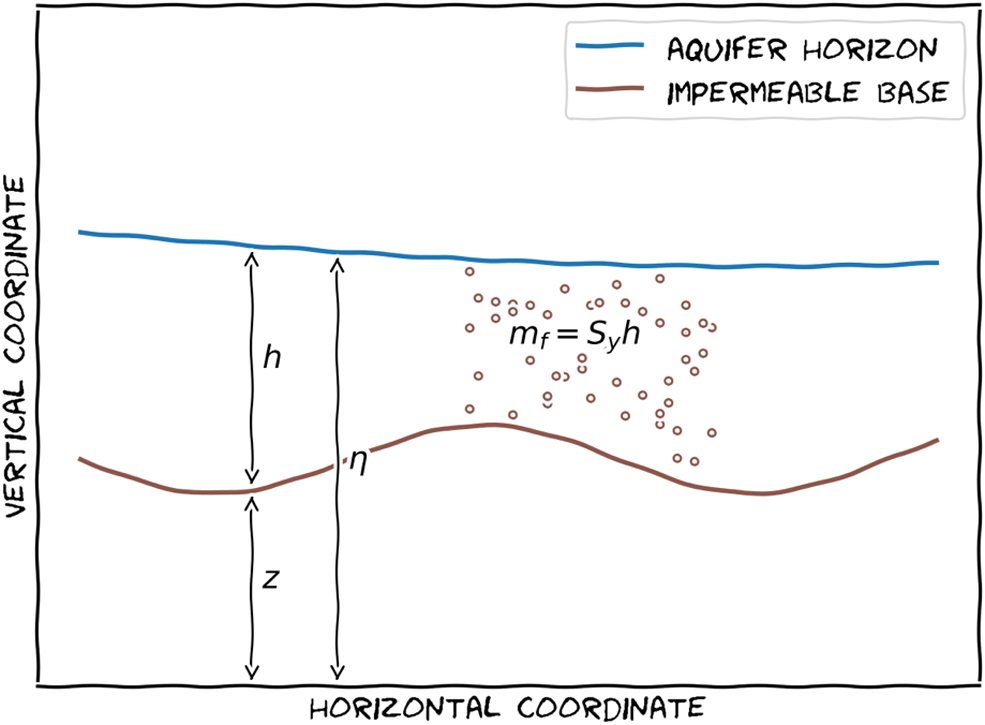
Definition sketch for the variables used in the BE and ADR. ADR, advection-diffusion-reaction equation; BE, Boussinesq groundwater flow equation.
Hyperbolic groundwater flow equation
Using Cattaneo's relaxation approach (Cattaneo, 1958), the first equation in Equation (1) can be written as a first-order hyperbolic system as:
where we have split η in the components h and z and used the chain rule to split the product of mf and Sy. τ is the relaxation parameter, and qf is the unit discharge of the fluid that converges to Kh∂xη as τ goes to zero. Thus, we may interpret the hyperbolization as a perturbation around an equilibrium state that corresponds to the original diffusion-type equation. Here, τ determines at what rate the hyperbolic system in Equation (4) relaxes toward its equilibrium state, that is to say the original diffusion-type equation. The smaller τ is, the faster the system converges.
Eq. (4) can be written in vector form as:
The eigenpairs of the coefficient matrix A are:
where λp is the p-th eigenvalue, and Rp is the associated p-th right eigenvector. Since all the eigenvalues are real and distinct, and the eigenvectors are linearly independent, Eq. (4) is strictly hyperbolic for all nonzero values of the relaxation parameter τ. The inverse of the column matrix of the right eigenvectors is:
Hyperbolic ADR
Application of Cattaneo's relaxation approach to the ADR has been reported in Toro and Montecinos (2014), and a hyperbolic pollutant transport equation is coupled to shallow flow equations in Vanzo et al. (2016). Similar to these references, the second equation in Equation (1) can be transformed as:
As τ goes to zero, ψc converges to ∂xc. Eq. (8) can be written in vector form as:
The Jacobian matrix of Eq. (8)—J = ∂QF—is computed as:
The eigenpairs of J are computed as:
D is always positive, and thus, all eigenvalues are real and distinct. The eigenvectors are linearly independent. Hence, Eq. (8) is hyperbolic for all nonzero values of τ. The inverse of the matrix of right eigenvectors is:
Numerical Scheme
Augmented Roe scheme
The governing equations are solved sequentially, using the augmented solver approach (Gosse, 2001; Murillo and Navas-Montilla, 2016) in fluctuation form. The cell average Qi in cell i at time level n is updated as:
where A±ΔQi±1/2 are the fluctuations, measuring the net effect of all ingoing waves. First, Eq. (4) is solved to provide the values of mf and qf, which are then used to solve Eq. (8).
Eq. (4) is formally a nonconservative system. A difficulty in finding weak solutions to nonconservative systems is that the nonconservative product A∂xQ is not well defined across discontinuities, even in a distribution sense (Parés, 2006). However, if the nonconservative product is integrated along a Lipschitz continuous path Ψ in phase space, it can be interpreted as a Borel measure (Dal Maso et al., 1995). Then, the fluctuations can be computed as:
and split into in- and outgoing fluctuations A±ΔQi±1/2 (LeVeque, 2011). A common path chosen in the literature is the linear path
which we use in this work to construct a Roe matrix as:
The definition of
In the classical wave propagation approach, the jump in the primary variables is split into waves (LeVeque, 2002); the augmented solver approach extends the definition of these waves to incorporate the source terms as:
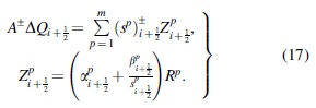
sp is the wave speed of the th wave, αp is the wave strength of the pth wave, and βp is the source strength of the pth wave (Murillo and Navas-Montilla, 2016). These values are computed by using the eigenpairs
Api±1/2 is calculated as the pth component of the vector:
where
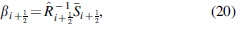
with
The numerical solution of Eq. (8) follows the same methodology. The major difference is that Eq. (8) is formally conservative. Thus, the Jacobian matrix can be linearized in the sense of Roe (1981) by using the classical Rankine-Hugoniot condition—see Roe (1981) and LeVeque (2002) for a discussion on Roe linearizations. This gives:
Source term discretization
We calculate the source terms through weighted averages of the conserved variables, proportional to the wave strengths as:
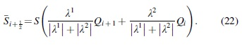
In this work, we use an arithmetic average for model parameters such as hydraulic conductivity, but other averages such as the harmonic average are also possible. This might be desirable, for example, if the difference in K between two cells is large.
Boundary conditions
We use ghost cells to impose boundary conditions. We define either water depth or discharge in the ghost cell and compute the other boundary value through finite differencing.
Depth boundary condition
If we impose the mass, mf,*, in the ghost cell—and thus, hf,* is known—the unit discharge in the ghost cell, qf,*, is calculated through Darcy's law as:
where the subscript i denotes values in the inner cell.
Inflow boundary condition
Similarly, if qf,* is imposed, the depth can be computed through Darcy's law as:
Species concentration boundary condition
If we impose the species concentration c, we can make use of the fact that lim
τ→0ψc
= ∂xc to compute the auxiliary variable, ψc, in the ghost cell through a forward difference as:
Comparison between parabolic and hyperbolic time step size
In this section, we only discuss the time step size for the hBE. The discussion of the time step size for the hADR is similar, but involves advective terms, which may be limiting the time step size more significantly than the diffusion terms. In such advection-dominated cases, the hyperbolization does not influence the time step size.
The efficiency of the hBE given in Eq. (4) can be assessed by comparing its eligible time step size with the parabolic equation's time step size, which can be constrained by a von Neumann stability analysis. Under the assumption of close to linear behavior from Equation (1), the eligible time step size can be estimated, such as in Hunter et al. (2005) and Caviedes-Voullième et al. (2013) as:
This assumption is valid for small gradients of the potential h. Due to the linearization, this constraint might be more restrictive than actually required. Nevertheless, it can be used as a first estimation. The eligible time step size of Eq. (4) is given by the classical CFL condition as:
The hyperbolic equation is more efficient than the parabolic one in terms of time step size if:
Using Equations (26) and (27) in Equation (28) and solving for τ gives a lower bound for the relaxation parameter τ as:
Thus, if values of τ that satisfy Equation (29) are still small enough to ensure that the hyperbolic system in Equation (4) converges to the parabolic Equation (1) in each time step, using the hyperbolic form is more advantageous.
Model Verification
In the following, we present a complete set of steady-state and transient benchmarks to verify the numerical scheme for both the hBE and hADR. In test cases without an analytical solution, we obtain the reference solution numerically using the ReacTran package (Soetaert and Meysman, 2019)—an R language package for numerically solving general ADR. In all test cases involving the BE, the relaxation time was set to τ = 0.2 Δx, which satisfies Equation (29). In test cases involving the ADR, we use the same τ as for the cases involving the BE, but here, the advection terms determine the time step size. The mesh resolution used in all test cases is sufficiently fine to obtain solutions in the asymptotic range. L∞-norm errors for all test cases are summarized in Appendix A1. Further, results from a mesh convergence study are reported in Appendix A1.
Subsurface flow test cases
Steady-state test cases
We run two simulations until they converge to a steady state, to verify that the steady states are correctly reproduced without spurious oscillations. The computational domain for all cases is L = 10 m long. At the upstream boundary, a constant inflow of q(x = 0) = 1 m2/s is imposed. The downstream boundary condition imposes a fixed fluid depth equal to the analytical solution at this location. The CFL number for all simulations is set to 0.9. Table 1 summarizes the relevant simulation parameters for all steady-state test cases. For each test case, model predictions are compared against an analytical solution—see Appendix A2 for the derivation.
Test Cases for hBE: Summary of Relevant Simulation Parameters
f(x) = exp(−2(x − 4)2) if x < 7, 1.5 if 7 < x < 8, 0 else.
Figure 2 shows the results for the water depth h for each of these simulations. Model predictions using 500 cells are plotted with circles. The continuous line shows the reference solution. We omit a plot of the unit discharge q for these test cases, as q converges to the analytical solution of constant 1 m2/s up to machine accuracy in each test case—we compute an L∞-norm <10−14 m2/s. The results prove that the numerical scheme preserves the discharge in moving equilibria up to machine accuracy in the presence of spatially varying conductivity and specific yield values. As seen in test cases BE3 and BE4, sharp discontinuities in the bed elevation z are handled well.
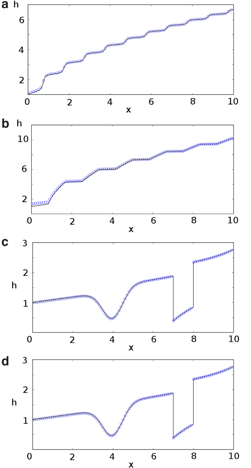
Steady-state test cases for hBE: Model prediction (circles) and analytical solution (continuous line) or h.
Transient test case
We consider an initial value problem for the hBE in a domain with a length of L = 10 m. At initial time, the fluid mass is constant mf(t = 0) = 3 m. Relevant simulation parameters are given in Table 1, row BE5. We discretize the domain with 2,000 cells. Figure 3a shows model predictions and reference solutions at different time steps. The transient case is accurately reproduced by the augmented scheme.
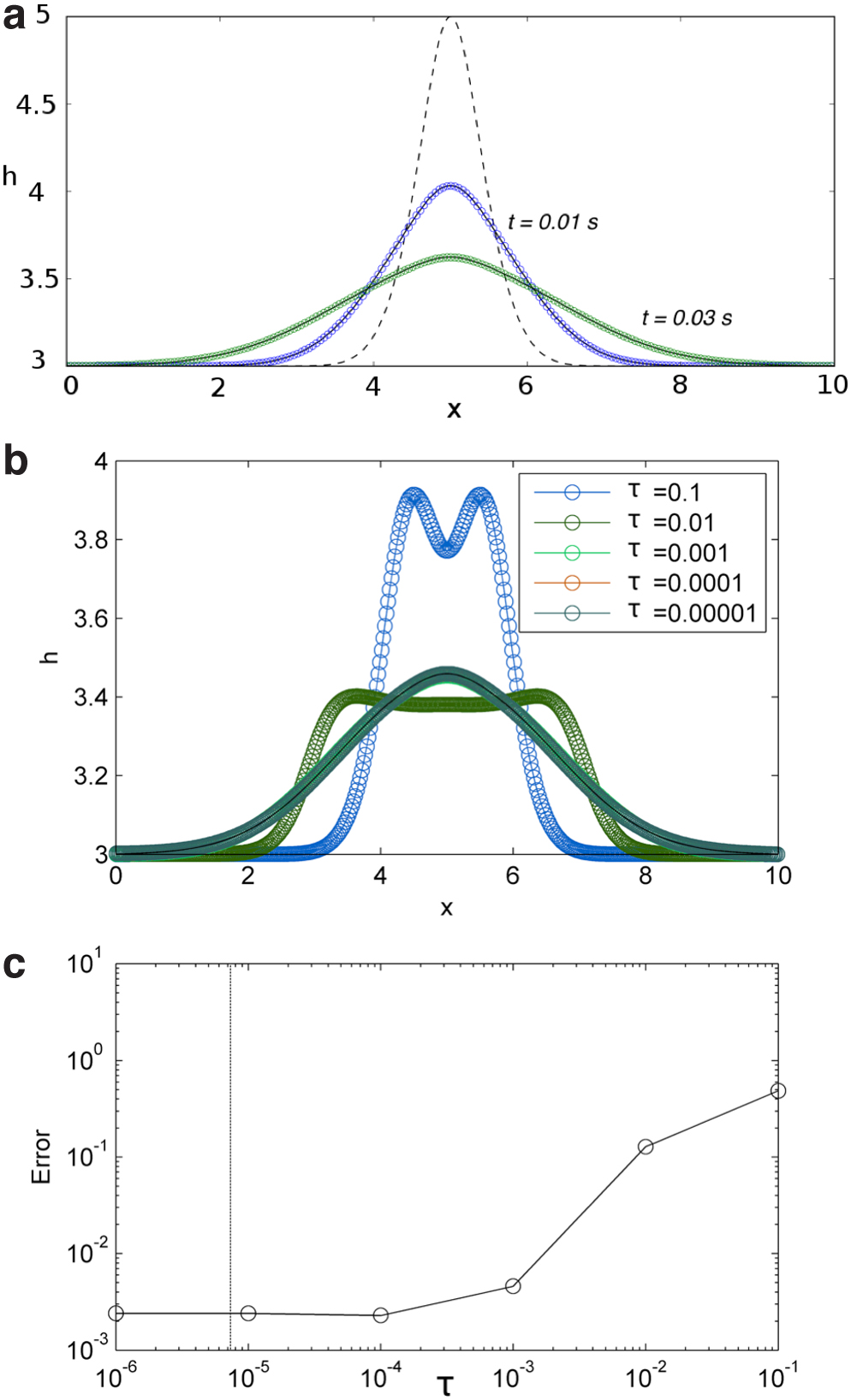
Transient test case for hBE: Model prediction (circles) and analytical solution (continuous line).
Using the same test case, we study the model's sensitivity to the relaxation time τ, which is varied from 10−5 to 0.1. Figure 3b shows model predictions and the reference solution for t = 0.03 s. Large values of τ, in this specific case in the order of magnitude between 0.01 and 0.1, result in large deviations from the reference solution. As τ is decreased below 0.001, the model predictions converge to the reference solution.
As the value τ affects the time step size, see Equation (27), it is desirable to choose τ as large as possible. Similar to the choice of mesh resolution, this results in a trade-off between efficiency and accuracy. Figure 3c plots the L∞-normed error against the value of τ. The dashed line marks the value where the parabolic time step is reached, see Equation (26). Values of τ below this line result in less efficient time steps compared with the original BE. Consequently, values of τ above this line ensure the hBE is more efficient than the BE. In our specific case, no significant improvement is gained after τ = 10−4.
Reactive transport test cases
Steady-state test cases
We run two simulations until they reach a steady state. The domain is L = 25 m long. A constant species concentration of c(x = 0) = 1 is injected at the boundary at x = 0. The concentration is reduced by a nonlinear reaction term along the domain. We discretize the domain with 500 cells. The constant injection at the boundary ensures that the system converges toward a steady state. We give the relevant simulation parameters in Table 2, rows ADR1 and ADR2. Figure 4 shows that our scheme completely reproduces the reference solutions for c at the steady state. Both test cases yield very similar results, because the advection dominates in both cases—the Peclet number is Pe ≫ 1 in both cases.
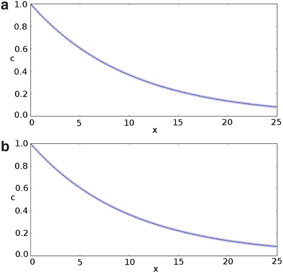
Steady-state test case for hADR: Model prediction (circles) and analytical solution (continuous line) for c.
Test Cases for hADR: Summary of Relevant Simulation Parameters
Transient test cases
We run transient simulation cases in a domain with length L = 100 m, discretized with 1,000 cells. We use periodic boundary conditions. Thus, simulation results only depend on the initial conditions, which are summarized in Table 2 for different simulation runs. In Table 2, ADR3 is a pure advection case, ADR4 is a pure diffusion case, ADR5 is an advection-reaction case, and finally, ADR6 is a full advection-diffusion-reaction case. For these cases, the analytical solution can be obtained as discussed in Appendix A2. A. In all cases, the analytical solution (continuous line) is captured satisfactorily (Fig. 5).
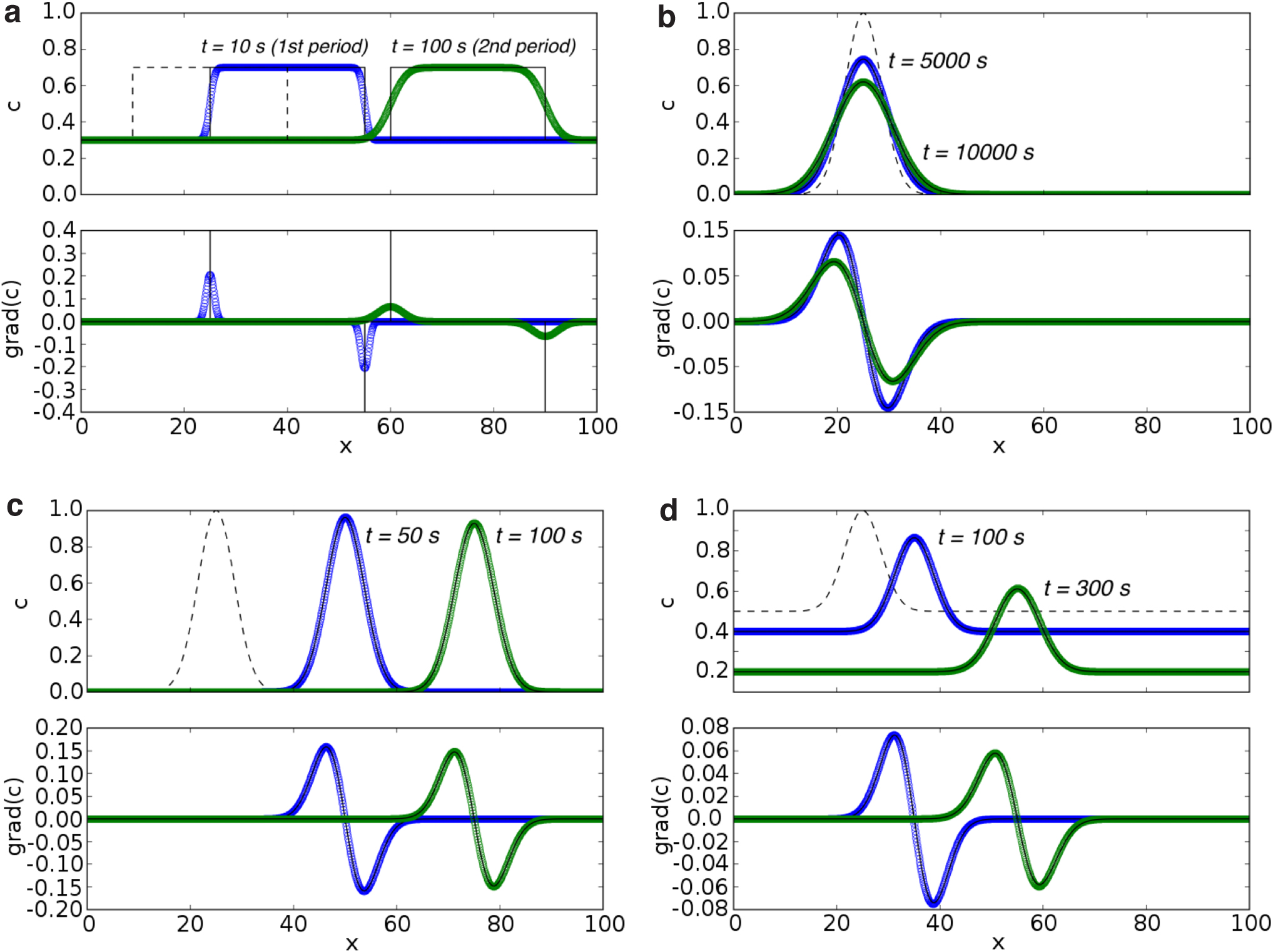
Transient test cases for hADR: Model prediction (circles) and analytical solution (continuous line) for c and ψc [grad(c)]
Modeling Intrameander Hyporheic Flow and Transport
We present a simulation of hyporheic flow and transport through a 62 m-long transect across a meander of the East River, Colorado (Fig. 6a). This transect has been studied in Dwivedi et al. (2018) to quantify geochemical exports from the hyporheic zone to the river. River water with high oxygen and nitrate concentrations enters the transect on the western boundary. The oxygen and nitrate are consumed in the hyporheic zone due to the presence of organic carbon sources, and they are exported back to the river on the eastern boundary. Figure 6a also shows the location of four measurement points where we compare our model predictions. The surface elevation is based on a digital elevation model with 0.5 m resolution (Wainwright and Williams, 2017).
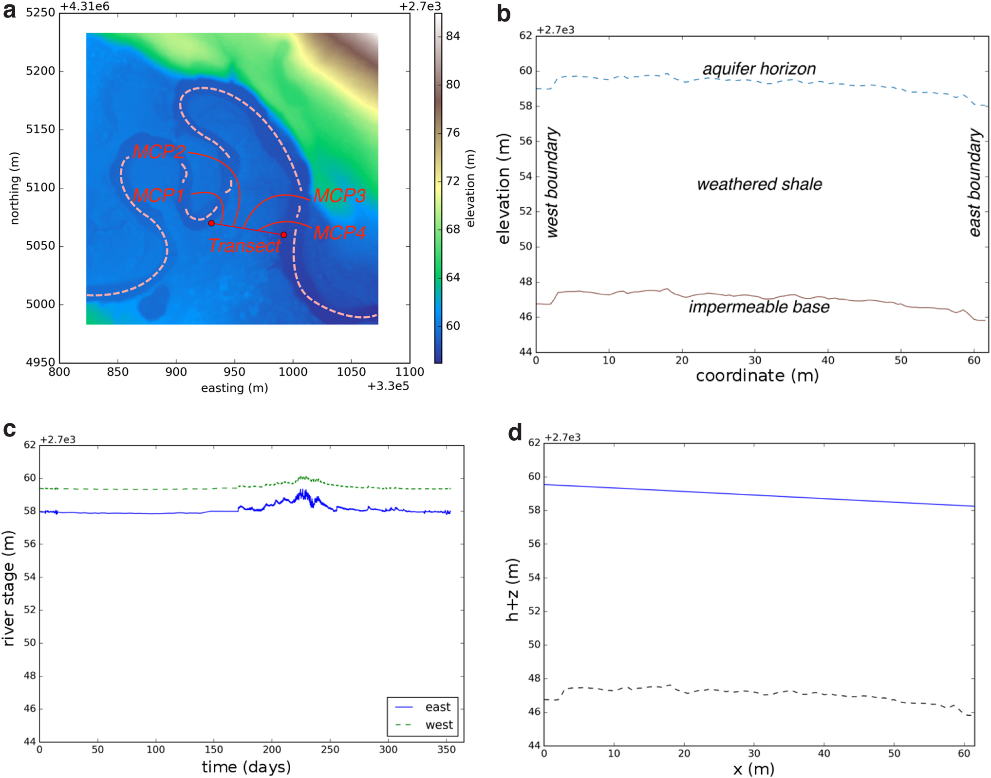
Intrameander hyporheic flow and transport: Study site and boundary and initial conditions.
The geology of the transect consists of three distinct layers (Dwivedi et al., 2018). The top layer is a 0.5 m-deep soil layer with low hydraulic conductivity, followed by a 1 m-deep gravel layer with high hydraulic conductivity. The third layer, which makes up the majority of the domain, is a weathered shale layer with low hydraulic conductivity. Our depth-averaged model is unable to resolve vertical heterogeneity in permeability. Hence, we assume that the permeable subsurface consists of weathered shale and that the impermeable boundary is below the surface (Fig. 6b). Based on field investigations (Tokunaga et al., 2019), the hydraulic conductivity of the weathered shale is set to K = 1.1 × 10⁻⁵ m/s. The transect is discretized with 124 cells with a resolution of 0.5 m, which corresponds to the data resolution. Using finer grids does not significantly improve the model predictions.
We obtain the initial conditions by running the model toward a steady state, using annually averaged constant head boundary conditions on both sides. Figure 6c shows the time series that we averaged to get the head boundary conditions. The difference in the piezometric head creates a hydraulic gradient, which drives the flow through the subsurface transect. Figure 6d shows the initial conditions we obtained. Our model predicts an average groundwater velocity of about vf = 2.3 × 10⁻⁷ m/s, which is an order of magnitude slower than the minimum velocity of vf = 5 × 10⁻⁶ m/s predicted in Dwivedi et al. (2018). The difference in model predictions is because our model is based on simplified physics and geology, whereas the model in Dwivedi et al. (2018) solves the three-dimensional Richards equation in a domain with several distinct vertical geological layers.
We apply the time series shown in Fig. 6c as head boundary conditions on both sides of the domain and simulate the transport of a dissolved electron acceptor (e.g., oxygen or nitrate) through the intrameander hyporheic zone. We use a diffusion coefficient of D = 10−3 m2/s, chosen rather high to qualitatively account for mechanical dispersion. We assume the electron acceptor to be consumed at the rate R = CcO, where C is a first-order reaction rate coefficient and cO is the dissolved concentration. The reaction rate coefficient accounts for the combined effect of the microbial community composition, the amount of organic carbon and other components, and the mineral composition in the soil (see, e.g., (Krause et al., 2013; Naranjo et al., 2015; Dwivedi et al., 2018). In this study, we choose C = 10−5 1/s as it results in complete consumption of the electron acceptor within the meander, which is consistent with observations in Dwivedi et al. (2018). We assume an initial concentration of cO(t = 0) = 0 in the entire domain and use a fixed concentration of cO(x = 0) = 0.25 at the upstream (western) boundary.
Figure 7 shows the model predictions for piezometric head against field measurements. The agreement is fair, and the overall dynamics of the measured piezometric head are captured by the model. Overall, the agreement gets worse as the flow propagates through the domain. This is most likely due to numerical diffusion and an incomplete representation of the physics. The agreement at MCP1 is the best, because its location is close to the boundary and is therefore less affected by numerical diffusion. At the other locations, the predicted curve lags behind the measurement and does not reproduce the peak accurately. High-frequency fluctuations are smoothed out by the model prediction. This may be a consequence of the simplified geology. Our model considers the entire domain to be shale. In reality, the top of the domain consists of a more permeable gravel layer, which may be responsible for the higher frequencies observed in the measurement data. Although model predictions might be further improved by modifying the conductivity to account for the top layers, the current predictions are sufficiently accurate for our purpose of presenting a proof-of-concept modeling study.
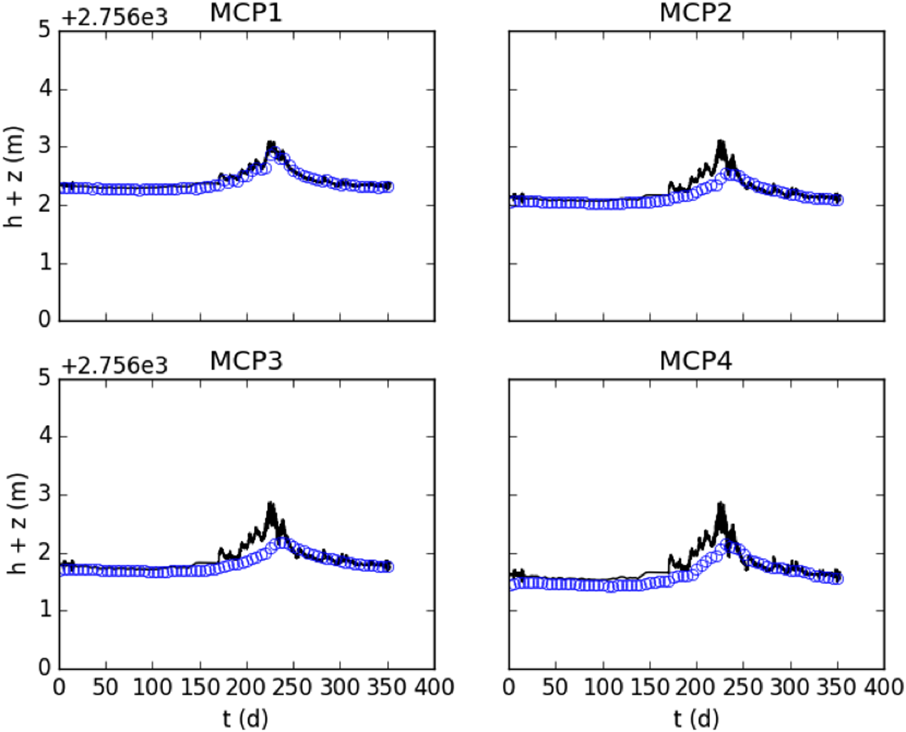
Intrameander hyporheic flow and transport: Model predictions (circles) and field measurements (continuous line) for piezometric head at 4 points along the transect.
Figure 8 shows model predictions for the electron acceptor concentration along the transect at different times. The electron acceptor concentration reaches a quasi-steady state at about 25 days, when the consumption balances out with the fluxes. The dynamics observed in the piezometric head in Fig. 7 does not significantly disturb this equilibrium, because the diffusive fluxes outweigh the advective fluxes. Although the model predictions qualitatively resemble the model predictions in Dwivedi et al. (2018), our hADR model with its simple reaction term is not comparable to the biogeochemical reaction network model utilized therein.
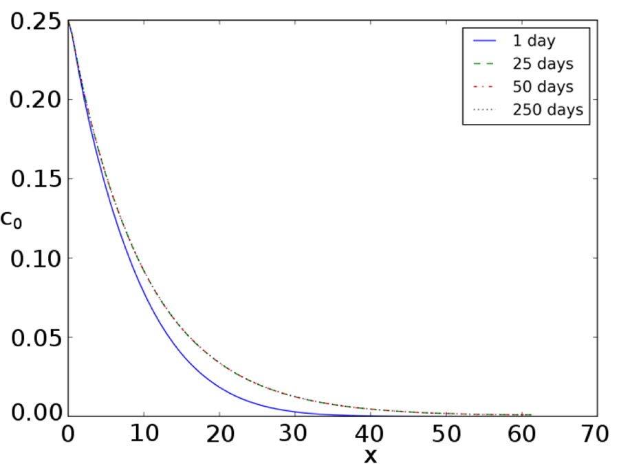
Intrameander hyporheic flow and transport: Model predictions for dissolved electron acceptor concentration along the transect at different times.
Conclusions
We applied Cattaneo's relaxation approach (Cattaneo, 1958) to the BE and the diffusive terms of the ADR. This transforms both equations into first-order hyperbolic systems with source terms. We used the augmented solver approach (Gosse, 2001; Murillo and Navas-Montilla, 2016), combined with a geometric reinterpretation of the source terms, to solve the hyperbolic system of PDEs.
Transient and steady-state benchmark test cases show that the relaxed hyperbolic system is equivalent to the original parabolic equations. The unit discharge in the BE appears as a primary variable in the hyperbolized equations. The numerical scheme enables us to compute the steady-state unit discharge with machine accuracy. These properties are desirable for coupled reactive transport simulations, because the advective flux in the ADR is determined by the unit discharge in the BE.
The case study of intrameander groundwater flow and reactive transport shows that the model is capable of modeling real-world cases to some extent. The depth-averaged groundwater flow model is unable to reproduce the fast component of the subsurface flow, but the overall dynamics are accurately modeled. The groundwater flow model can be extended to higher dimensions to overcome the limitations of depth-averaged modeling. The coupled ADR computes feasible results but suffers from an even more simplified representation of the processes. The case study serves as a proof of concept, and the reaction terms can be computed in a more sophisticated manner if needed. Adding more species to the model for multi-component reactive transport simulations is straight-forward, but it has not been explored in this work.
Overall, using Cattaneo's relaxation approach to hyperbolize parabolic governing equations and using an augmented solver to numerically solve the resulting hyperbolic system is shown to be a viable approach. The presented method can be applied to other areas of hydrological modeling that are governed by parabolic equations. However, additional studies are necessary to completely assess the advantages and limitations of this method for hydrological applications.
Footnotes
Author Disclosure Statement
No competing financial interests exist.
Funding Information
This work is supported as part of the Watershed Function Scientific Focus Area funded by the U.S. Department of Energy, Office of Science, Office of Biological and Environmental Research under Award Number DE-AC02-05CH11231. This work is supported as part of the Interoperable Design of Extreme-scale Application Software (IDEAS) by the U.S. Department of Energy, Office of Science, Office of Biological and Environmental Research, Award Number DE-AC02-05CH11231. A.N.-M. is partially funded through Gobierno de Aragón through the Fondo Social Europeo. The data of the case study is based on work supported as part of the Sustainable Systems Scientific Focus Area, funded by the U.S. Department of Energy, Office of Science, Office of Biological and Environmental Research under Award Number DE-AC02-05CH11231.