Do Family Dinners Reduce the Risk for Early Adolescent Substance Use? A Propensity Score Analysis

Abstract

The risks of early adolescent substance use on health and well-being are well documented. In recent years, several experts have claimed that a simple preventive measure for these behaviors is for families to share evening meals. In this study, we use data from the 1997 National Longitudinal Study of Youth (n = 5,419) to estimate propensity score models designed to match on a set of covariates and predict early adolescent substance use frequency and initiation. The results indicate that family dinners are not generally associated with alcohol or cigarette use or with drug use initiation. However, a continuous measure of family dinners is modestly associated with marijuana frequency, thus suggesting a potential causal impact. These results show that family dinners may help prevent one form of substance use in the short term but do not generally affect substance use initiation or alcohol and cigarette use.

Keywords

adolescent health adolescent substance use family dinners matching propensity score

The risks of early adolescent substance use are well documented. Those who begin to use alcohol, tobacco, or other drugs early in life are at heightened risk for delinquent and criminal behavior, premature adult transitions, impaired educational achievement, limited occupational opportunities, and poor emotional and physical health (e.g., Green and Ritter 2000; Krohn, Lizotte, and Perez 1997; Wiesner, Kim, and Capaldi 2005). Thus, it is not surprising that numerous ideas about how to inhibit this behavior have been promoted. In fact, there is no shortage of programs designed to prevent adolescent substance use (Ennett et al. 2003). These programs address various aspects of adolescent life and multiple characteristics because, it is thought, there is no single preventive measure for these types of risk behaviors (Ellickson et al. 2003).

Media attention and expert advice have, however, recently endorsed what appears to be a straightforward approach to drug prevention. Although mass marketing campaigns or police-led interventions have proved largely ineffective, according to several substance abuse and prevention experts a simple solution is for families to share meals (Eisenberg et al. 2008; National Center on Addiction and Substance Abuse 2012). They contend that if families have meals, especially evening meals, together, there is an opportunity to build family relationships and monitor adolescents’ activities. Assuming that shared meals offer these and other benefits, children may, as a consequence, be less likely to use illicit substances.

Research on family meals and adolescent substance use has yielded mixed results, however. Although several studies have found negative effects on adolescent substance use (e.g., Eisenberg et al. 2008; Fulkerson et al. 2006), recent research suggests that the association between family meals and substance use is likely due to other aspects of the family environment (Miller, Waldfogel, and Han 2012; Musick and Meier 2012). Nevertheless, most studies rely on empirical models that simply control for potential confounding variables or attempt to partial out time invariant factors. There has been no attempt to study the nonrandom assignment of families to shared meals and what this assignment process indicates about whether family meals have a causal impact on adolescent substance use. In general, the selection bias that affects the frequency of family meals has not been considered adequately in previous research.

In this study, we use propensity score matching models (Guo and Fraser 2010; Rosenbaum 2010) to attenuate selection bias so that the potential causal effects of family meals on adolescent drug use may be illuminated (cf. Slade et al. 2008). In particular, we examine the frequency of family meals as the treatment assignment and create matched samples on the basis of propensity scores established using a set of observed covariates. We then compare the expected values of substance use across the matched samples to determine the “treatment effect” (Stuart 2010). The propensity scores are estimated for binary, categorical, and continuous treatment distributions. This is vital because previous studies have not used consistent measurement strategies for family meals (cf. Eisenberg et al. 2008; Musick and Meier 2012), thus making it difficult to determine if there are continuous, discrete, or threshold effects on adolescent drug use. On the basis of recent studies, we hypothesize that family meals have no causal impact on early adolescent substance use. Instead, the ostensible effect of family meals is likely due to other characteristics of families that affect this behavior.

Background

Given the well-established risks of early substance use on subsequent health and well-being (e.g., Krohn et al. 1997; Wiesner et al. 2005), it is not surprising that much effort has been spent to determine the best way to prevent the onset or minimize the frequency of substance use among young adolescents. Although most scholars recognize that early involvement in drug use is the result of a complex interplay of intrapersonal, interpersonal, and macro-level influences (e.g., Brook et al. 2006; Hoffmann 2002), efforts to find discrete preventive measures continue unabated. For example, recent media marketing efforts such as the Office of National Drug Control Policy’s Marijuana Initiative are predicated on the assumption that relatively simple messages about the dangers of substance use are a sufficient deterrent for most adolescents (Hornik et al. 2008).

Although narrow approaches are not generally effective, an interesting recent attempt at promoting a singular solution involves family meals. Endorsed by both public policy advocates and prevention experts, the idea is that families that share meals more often develop the bonds necessary to deter involvement with illicit substances (Califano 2007; Eisenberg et al. 2008). Presumably, shared mealtimes produce this effect through several theoretical mechanisms that are familiar to adolescent researchers.

First, family meals offer parents an opportunity to connect with their children by enhancing attachments and allowing more time to talk and discuss their lives and concerns (Griffin et al. 2000). More frequent interaction during meals may also increase monitoring, as parents have opportunities to ask about their children’s friends and activities. Similarly, involvement and interaction with conventional others, such as most parents, should lead to the reinforcement of conventional behaviors (Catalano et al. 1996). Family mealtimes presumably offer parents a chance to not only interact with their children but also reinforce normative behaviors. Finally, family mealtimes are associated with lower levels of stress, which in turn may predict a decreased risk for illicit substance use (National Center on Addiction and Substance Abuse 2012).

Family meals are also a key type of normative, ritualized activity in Western society. These rituals encourage family interaction, allow children to feel acknowledged and recognized, and create and enrich family identity and traditions. Moreover, they offer a sense of family unity and build interpersonal connections that are important for adolescent development (Fiese, Foley, and Spagnola 2006).

These ostensible benefits and processes of family mealtimes have rarely been examined directly (see, however, Franko et al. 2008), but several studies have found that more frequent family meals are associated with positive adolescent development. This includes lower risks of precocious sexual activity, depressive symptomatology, antisocial behaviors, school problems, binge eating, and obesity (e.g., Fulkerson et al. 2006). They are also associated with less adolescent substance use contemporaneously and longitudinally, presumably because of the conceptual mechanisms discussed earlier (e.g., Eisenberg et al. 2008; Griffin et al. 2000). However, this may depend on the type of substance use examined (Sen 2010).

An important issue is whether family meals have a direct impact on adolescent substance use or whether this association is simply a consequence of a positive family environment. It is relatively well established that family environment and structure, in particular parent-child relations, parental monitoring, and related family factors, are associated with adolescent substance use (e.g., Bahr, Hoffmann, and Yang 2005; Repetti, Taylor, and Seeman 2002). More frequent family meals are also predicted by these and other family factors (e.g., high socioeconomic status, maternal employment) (Davidson and Gauthier 2010). Hence, it is not surprising that the positive effects of family meals are likely affected by whether children get along well with their parents and siblings (White and Halliwell 2010). Thus, aspects of the family environment may confound or otherwise account for the observed association between family meals and adolescent substance use.

In fact, recent research suggests that this is may be the case. A small number of studies indicate that the association between family meals and youth behaviors dissipates once other factors are considered, including parent-child relations, parental monitoring, and related factors (Miller et al. 2012; Musick and Meier 2012; White and Halliwell 2010). For example, after statistically adjusting for a spate of variables (e.g., parental involvement, family structure), Miller et al. (2012) found no statistically significant impact of the frequency of family meals on problem behaviors such as arguments and aggression among children in grades 5 and lower. However, they did not study adolescent behaviors.

Similarly, Musick and Meier (2012) used the National Longitudinal Study of Adolescent Health data set to examine substance use and other outcomes among adolescents aged 12 to 17, along with follow-up data when they were aged 18 to 26. In fixed-effects analyses, they found little evidence that family dinners attenuate involvement in substance use longitudinally. However, they did find modest negative influences of family dinners on the odds of substance use in a cross-sectional model. Importantly, though, Musick and Meier determined that adjusting for a host of covariates, including family relationships, conflict, and maternal employment, accounted for more than half of the family dinner effect. Although this research suggests that there is little, if any, causal connection between these variables, as described below, there are limitations to the fixed-effects regression models that have been used in recent studies.

In general, the evidence is mixed regarding whether family meals are an important influence on adolescent substance use. Although some research indicates that encouraging families to share meals is a promising impediment to adolescent substance use, a small number of recent studies casts doubt on this conclusion. Instead, they suggest that various aspects of the family environment may predict both the frequency of family meals and the risk for adolescent substance use, thus accounting for the associations found in earlier research.

In this study, we extend the research on this topic in three important ways. First, in contrast to past research, we operationalize family dinners in several different ways to determine if the potential effect on drug use differs because of the way this explanatory variable is assessed (e.g., linear vs. categorical). Second, we examine several measures of drug use: the frequency of alcohol, cigarette, and marijuana use and the initiation of use over a one-year period. This differs from several studies that have aggregated substance use. Third, we examine the association in an empirically distinct way than past studies by using three types of propensity score methods that are designed to estimate the causal impact of family dinners on adolescent drug use. The following section discusses the propensity score approach in more detail.

Propensity Score Matching

Most research on family meals and adolescent substance use has used multivariate linear or logistic regression to estimate their empirical associations. An alternative has been to use fixed-effects regression models with longitudinal data to attenuate the bias that results from stationary unobserved variables; this presumably identifies potential causal effects (e.g., Musick and Meier 2012; Sen 2010). However, the causal modeling literature also advocates the use of matching techniques with observational data (Rosenbaum 2010; Stuart 2010). Studies indicate that fixed-effect estimators yield substantial bias and are relatively inefficient for capturing causal effects. Thus, propensity score matching is the recommended alternative because it leads to less bias in point estimates and is more efficient (Dehejia and Wahba 1999; Michalopoulos, Bloom, and Hill 2004; Rubin and Thomas 2000).

The most common matching approach is to establish comparable groups first through the use propensity scores, followed by a model that estimates differences in outcomes, such as substance use, across the groups (e.g., Slade et al. 2008). In general, the idea is to mimic experimental studies by constructing treatment and control groups, thus reducing the selection bias that is inherent in observational studies.

Specifically, it is a virtual certainty that the frequency of family meals is not randomly assigned across families (Davidson and Gauthier 2010). Thus, when examining its potential effects on substance use studies attempt to control for confounding variables (e.g., Eisenberg et al. 2008). But because we do not directly observe substance use among those who do share frequent family meals relative to their substance use if they did not share frequent family meals, we can never examine both potential outcomes for the same person. In other words, the counterfactual is never observed directly.

Researchers typically consider aggregated estimates as a substitute for individual (unobserved) estimates of the family meal effect. To move closer to a causally relevant model, however, we would have to assume that the average level of use for those who experience more family meals is equal to the average use for those who experience fewer family meals if they had experienced more family meals. Yet because selection bias affects the frequency of family meals, this assumption can rarely, if ever, be tested.

Given that we cannot directly observe the counterfactual condition, one solution is to study the nonrandom assignment mechanism—in this case the characteristics that affect family meal frequency. If we can establish a suitable model that predicts this assignment mechanism, we may use this information to (1) partial out the effects of observed covariates by creating treatment and control groups, and (2) estimate expected differences in substance use for these groups, thus estimating the average “treatment” effects of family meals on substance use. An essential step of this approach is the creation of these groups. It is important that the groups closely resemble one another, just as randomization in experimental studies results in similar treatment and control groups. A commonly used approach is to develop a prediction model of the assignment process and then estimate the propensity score, or the conditional probability of treatment given a set of observed covariates: [p(x) = Pr(T = 1 | x)]. A key feature of this is that individuals with the same propensity score, whether they fall in the observed treatment or control group, have the same distribution of the observed covariates. This is known as the balancing property (Rosenbaum and Rubin 1983). Thus, assuming that a good estimate of the true propensity score is found, comparable treatment and control groups that are balanced on a set of covariates may be identified (Rosenbaum 2010).

Next, we may substitute those observed on the same set of covariates for those unobserved to get the expected effect for the counterfactual case. This is done by averaging over units to get the aggregated estimate of the treatment effect. Although matching leads to a modest loss in efficiency, research suggests that matched samples balanced by propensity scores provide estimates with less bias and greater efficiency than linear regression estimates or fixed-effects estimators on the basis of unmatched samples (Dehejia and Wahba 1999, 2002; Rubin and Thomas 2000).

In this study, we use a nationally representative sample of young adolescents to explore the potential causal impact of family dinners on the frequency and onset of substance use. In particular, we develop a selection model on the basis of an extensive set of predictors to account for the nonrandom assignment of these adolescents to different levels of family dinner frequency. The estimated propensity scores from this model are then used to create matched treatment and control samples. Next, we compare the predicted odds of substance use initiation and the estimated means of alcohol, tobacco, and marijuana use across the groups to determine whether there are differences. We also consider family dinner frequency as a binary, categorical, and continuous indicator, thus establishing whether the potential causal effects on substance use depend on the way it is measured.

Data and Methods

The data used to test the empirical models are from the 1997 National Longitudinal Study of Youth (NLSY97). The NLSY97 began in 1997 with a sample of 6,748 adolescent respondents who represented the population of 12- to 16-year-olds in the United States. The survey includes extensive information on demographic characteristics and the use of alcohol, cigarettes, and marijuana. Technical details on the sample design and interview protocol are available in the NLSY97 User’s Guide (Center for Human Resource Research 2004).

Because relevant questions concerning family dinners, parent-child relations, and family behaviors are limited to respondents aged 12 to 14 years during the first year of data collection (Center for Human Resource Research and Child Trends 1999), we limit our analysis to this early adolescent subsample and the first two waves (1997–1998). Because of this restriction, the analytic sample, ignoring variations in item nonresponse, is 5,417 for wave 1. There was about 6 percent attrition from wave 1 to wave 2, with about 5,074 respondents completing the 1998 survey. Analyses indicate few systematic differences in family of origin or adolescent outcomes due to attrition (Aughinbaugh and Gardecki 2007).

As with any large data set, there is item nonresponse. Although most of the variables had less than 5 percent missing, about 20 percent of respondents were missing data on family income. To obviate analytic problems associated with missing data, we estimate a multiple imputation model. A chained equation method is used to generate 25 imputed data sets (Van Buuren et al. 2006). The imputation model includes all variables in the subsequent analyses, along with several auxiliary variables (e.g., some parenting items, grade in school, parent religiosity). Although there are questions regarding whether imputed values of outcome variables should be included in subsequent analyses (von Hippel 2007), biases are more likely to be absent with the use of auxiliary variables in the imputation model. We estimated the models with and without imputed outcome variables. Because our conclusions regarding the impact of family dinners do not change across these models, we present the results with the imputed outcome variables.

Measures

Previous research on adolescent drug use has used different scales, including binary indicators (e.g., no use vs. use), discrete categories, or continuous variables (e.g., past 30-day frequency of use). Several scholars argue that continuous measures are most appropriate, because more frequent use is associated with subsequent problem use and other health consequences (e.g., Bahr et al. 2005). Binary measures tend to conflate those who use only occasionally with those who use more often (Macleod et al. 2004). Moreover, studies have addressed initiation of use because its predictors may differ from those that predict the frequency of use, and preventing initiation during adolescence is a key goal of most intervention programs (Kosterman et al. 2000). We therefore rely on continuous measures of three of the most common types of drug use: alcohol use frequency in the past 30 days, cigarette use frequency in the past 30 days, and marijuana use frequency in the past 30 days. Moreover, drug use initiation, or whether respondents initiated substance use between 1997 and 1998, is also examined.

The variables concerning past 30-day use are based on the following questions: “Have you ever used [substance]?” and, for those who answered “yes,” “On how many days have you used [substance] in the last 30 days?” We combined responses to these two sets of questions to create past 30-day frequency variables. Because the frequency items are highly skewed, the natural logarithm of each (+1) was computed and used as outcome variables. The NLSY97 database includes constructed variables for waves 1 and 2 that measure any use of the aforementioned substances. By manipulating these variables, we constructed a categorical measure of initiation versus three other outcomes. Those who reported no lifetime use in 1997 yet reported use of any of these substances in 1998 are identified as initiators, whereas those who did not use in either year are identified as abstainers. The other two categories are those who stopped using and those who continued to use, but we limit our attention to initiation versus abstention.

The key explanatory variable is family dinners. Unfortunately, there is a lack of consistency in how family dinners have been measured. Some have considered categorical indicators of family dinner frequency (e.g., Eisenberg et al. 2008), whereas others have used continuous measures (e.g., Sen 2010). Both have strengths and weaknesses, however. Categorical measures may yield different results depending on the cut points used. Continuous measures may fail to show threshold effects or may mask nonlinearities in the associations. Because there is no clear guidance and we wish to offer a comprehensive view of the potential effects of family dinners, we use two categorical measures and a continuous measure. All of them are based on the following question: “In a typical week, how many days from 0 to 7 do you eat dinner with your family?”

Following Eisenberg et al. (2008), we first create a binary measure, with zero to four days as a low-frequency group and five to seven as a high frequency group. This scheme is used in the propensity score models that address binary treatment. An alternative categorical approach has been to identify three classes of frequency: zero to two days, three to five days, and six to seven days (Fulkerson et al. 2006). We adopt this coding strategy for the categorical treatment models. Finally, recent studies have treated family dinners as a continuous variable, zero to seven days a week (e.g., Musick and Meier 2012; Sen 2010). This coding strategy is used in the generalized propensity score models described later.

As mentioned in the section on sensitivity analyses, several other measurement approaches were also considered, such as a binary variable coded as zero to six days versus seven days and a categorical measure coded as zero to three days, four to six days, and seven days. In addition, because family dinner frequency manifests high negative skew, we estimated models with transformations in an attempt to induce normality. However, none of these approaches yields substantially different empirical results, so the three measures described earlier are used.

Because a key concern is to predict “treatment assignment” (frequency of family dinners) and subsequently examine whether it predicts substance use, we use two overlapping sets of covariates: those that research suggests influence family dinner frequency or affect adolescent substance use. Studies indicate that shared family dinners are predicted by gender, race-ethnicity, family income, parental education, mother’s employment, age, family structure, size of household, time use by adolescents, religiosity, and parent-child relations (e.g., Davidson and Gauthier 2010; Tepper 2001).

Several of these variables are also common predictors of adolescent substance use (e.g., Bailey and Hubbard 1990; Brook et al. 2006). In addition, substance use is consistently associated with parental monitoring, the surrounding physical environment, and peer behaviors (Allen et al. 2003; Hoffmann 2002; Kosterman et al. 2000).

We use several variables to construct measures of parent-child relations and parental monitoring. Parent-child relations are based on a scale developed by Child Trends (Hair et al. 2008). The scale is based on 16 questions that ask respondents about their mothers and fathers. The questions include inquiries such as “I really enjoy spending time with him/her,” “How often does s/he praise you for doing well?,” and “How often does s/he criticize you or your ideas?” Depending on the particular question, response options include “never” (coded 0) to “always” (coded 4) and “strongly disagree” (coded 0) to “strongly agree” (coded 4). Higher values on this scale indicate a closer relationship with one’s parent. Cronbach’s α values for the mother and father sets of responses are .78 and .82. Because some adolescents, especially those living with single parents, did not respond to these questions for both parents, we use the following scheme to retain as much information as available. If adolescents provided responses to these questions for both mothers and fathers, we take the average of the two response sets. If responses were available for only one parent, such as in single-parent families, we use the mean of that response set.

Parental monitoring was the composite of several items that asked how much the adolescent’s parents know about (1) his or her friends, (2) his or her close friends’ parents, (3) who he or she is with when not at home, and (4) his or her teachers and school activities. Responses range from “knows nothing” (coded 0) to “knows everything” (coded 4) (Hair et al. 2008). The monitoring scales have Cronbach’s α values of .76 (mother) and .82 (father). As with parent-child relations, we retain as much information as available by taking the mean of the two response sets about mothers and fathers if both are available or the mean of the response set if available for only one parent.

Time use is based on a series of questions that asked how many weekdays the youth spent doing homework, watching television, and reading for pleasure. Another question asked how many days in the previous week one’s family did something “fun such as play a game, go to a sporting event, and so forth.” A similar question inquired about doing “something religious as a family such as go to church, pray or read the scriptures together?” The first three variables are coded zero to five days, whereas the next two are coded as zero to seven days. Finally, days absent from school asked about the previous school term or semester. Because it manifests high positive skew, we log-transformed it after adding 1 to preserve the zeros (skewness of transformed variable = .21).

Physical environment is a composite measure based on a set of questions that asked about electricity in the home, the interior of the home, the condition of buildings in the neighborhood, whether the residential area is safe, and whether respondents had heard gunshots in a typical week. The items are summed to produce a composite score, with higher values indicating a more risky physical environment (Center for Human Resource Research and Child Trends 1999).

Peer substance use is based on a set of questions that asked adolescent respondents to estimate the percentage of youth in their grades at school who smoked cigarettes, got drunk at least once a month, and used marijuana, inhalants, or other drugs. The response categories range from “almost none (less than 10 percent)” (coded 1) to “almost all (more than 90 percent)” (coded 5). A limitation of these variables is that they do not directly measure friends’ behaviors; they only represent one’s perceived peer environment (Allen et al. 2003). Nevertheless, recent research suggests that beliefs about peer substance use are at least as important as actual peer behaviors among early adolescents (Nargiso, Friend, and Florin forthcoming).

The demographic variables are taken from the youth and parent or head of household NLSY97 surveys. Gender is coded as 1 = female and 0 = male. Some studies have shown that family meals are more consequential for girls (e.g., Eisenberg et al. 2008), but supplementary analyses indicate that this is not applicable to these data. Thus, we simply control for gender in each model (cf. Musick and Meier 2012). Age is coded in years, 12 to 14. Race-ethnicity involves a set of four dummy variables available in the NLSY97: white or other racial or ethnic status, African American, Hispanic, and mixed race-ethnicity. Residence is also a set of three dummy variables: urban or suburban, rural, and unknown. Family structure is measured with a set of four dummy variables: two–biological parent family, stepparent family, single-parent family, and other family type.

Size of household identifies the number of family members who lived in the home. It ranges from 1 to 12, with a mean of 2.44. Parental education is coded in years and indexes the highest level of education among either parent (M = 13.66 years). Mother’s employment is based on the roster of household members and is coded as 0 = mother not employed outside the home and 1 = mother employed outside the home. Family income is measured in dollars and gauges past-year income from all sources. Given its positive skew, we use the square root to normalize its distribution (skewness of transformed variable = .58). Table 1 provides summary information for the outcome and explanatory variables. Note that a majority of respondents reported six or seven family dinners per week.

Table 1.

Descriptive Statistics, 1997 National Longitudinal Study of Youth.

Variable	M or Proportion	SE	Minimum	Maximum
Frequency of family dinners	5.19	.03	0	7
Binary frequency of family dinners (0–4 vs. 5–7 days)	.72	.01	0	1
Categorical frequency of family dinners
0–2	.14	.02
3–5	.30	.01
6–7	.56	.01
Substance use, 1997
Past 30-day alcohol use, logged	.15	.01	0	3.4
Past 30-day cigarette use, logged	.28	.01	0	3.4
Past 30-days marijuana use, logged	.08	.01	0	3.4
Substance use, 1997–1998
Abstained from use	.39	.01
Initiated use	.17	.01
Stopped using	.10	.02
Continued to use	.33	.01
Female	.49	.01	0	1
Age (years)	13.00	.01	12	14
Race-ethnicity
White/other	.71	.01	0	1
African American	.15	.01	0	1
Hispanic	.13	.02	0	1
Mixed race-ethnicity	.01	.02	0	1
Residence type
Urban/suburban residence	.69	.01	0	1
Rural residence	.26	.01	0	1
Residence unknown	.05	.02	0	1
Family structure
Two–biological parent family	.54	.02	0	1
Stepparent family	.14	.01	0	1
Single-parent family	.27	.01	0	1
Other family type	.05	.02	0	1
Size of household	2.44	.02	1	12
Family income, square root	207.68	1.35	0	496
Parental education	13.66	.04	1	21
Mother employed	.57	.01	0	1
Weekdays did homework	3.46	.02	0	5
Weekdays read for pleasure	1.91	.03	0	5
Weekdays watched television	4.30	.02	0	5
Days family did fun activities	2.68	.03	0	7
Days family did religious activities	1.54	.03	0	7
Days absent from school, logged	1.25	.01	0	5
Parental monitoring	9.57	.05	0	20
Parent-child relations	24.92	.07	0	34
Physical environment	11.87	2.00	0	70
Peers who smoke	2.26	.02	1	5
Peers who get drunk	1.69	.02	1	5
Peers who use illegal drugs	1.90	.02	1	5

Note: Means and proportions are averages estimated across 25 multiply imputed samples and are based on weighted data; n = 5,419.

Analytic Methods

Our goal is to estimate the effect of family dinners on adolescent substance use using propensity score matching and weighting. However, as discussed earlier, previous studies have not identified a standard way to measure family dinners. Thus, we use several propensity score matching models in this study. The first type is appropriate when the treatment variable, family dinners, is binary (zero to four vs. five to seven days) or continuous (zero to seven days). In this approach, the first step is to estimate a statistical model that predicts family dinner frequency. For the binary indicator, we use a probit regression model (Stuart 2010) and for the continuous variable, we use a generalized propensity score model (also called a dose-response model), which is based on the standard normal density function (Hirano and Imbens 2004). The key to both of these is to estimate a selection model that accounts well for the assignment to the treatment categories. To meet the conditional independence assumption of these models, all potential variables that are related to processes of assignment into family dinner categories should be included in the model. Experts also recommend that one consider quadratic and interaction terms to better predict the treatment assignment. This is to satisfy the assumption of ignorable treatment assignment (Stuart 2010). To strengthen the predictive ability of models, we conducted a comprehensive assessment of the set of explanatory variables described earlier, along with quadratic terms for continuous covariates and interactions among sets of variables (cf. Slade et al. 2008). The decision rule was to include any covariate with a p value < .20 in the selection model. Two quadratic terms emerged as predictive of family dinners: parental monitoring squared and religious activities squared. Thus, each was included in the models. Moreover, only one of the peer variables was predictive—peers who get drunk—the other two peer variables were included only in the subsequent postmatching models.

Once the estimated propensity scores are determined from the probit or generalized models, they are used to match on the covariates that predict family dinner frequency. Similar to randomized experiments, the goal of matching is to achieve covariate balance or restrict the sample to a set of respondents who are comparable on these covariates. If comparisons indicate only modest mean or proportion differences among the covariates for the matched groups, then we may assume that these characteristics are not responsible for differences in outcomes across the groups. Although a number of matching methods are available, we use a nearest-neighbor model with replacement and limit the number of potential matches with a caliper for the binary treatment models (Dehejia and Wahba 2002). Various caliper levels were examined; a relatively small caliper (.005) is used on the basis of its ability to balance the covariates efficiently and maintain a substantial number of treatment and control cases. Up to five matches of controls to each treatment are specified to ensure adequate reliability across groups. The generalized propensity score model uses a blocking routine with cut points to match groups (Hirano and Imbens 2004). Following matching on covariates, we tested the balancing property for both types of models. This was followed by means/odds comparison tests based on linear or multinomial regression models to determine if the propensity of family dinners affects substance use. The most common approach is to focus on the average treatment effect on the treated, or the expected effect of family dinners on substance use for those experiencing more frequent family dinners.

The second type of model is appropriate for the three categories of family dinner (zero to two, three to five, and six or seven days). This also involves a prediction equation, in this case a multinomial logistic model, which is then used to calculate predicted propensity scores or the probability of falling into each category. The inverse of the scores are used as sampling weights in linear or multinomial regression models designed to predict the outcomes (Guo and Fraser 2010). A presumed benefit of this approach is that it uses all the data, rather than discarding cases that cannot be matched to a treatment unit. A disadvantage is that it includes observations outside the common support area.

Postmatching adjustment

Although most studies compare expected values across matched groups to determine the causal impact of treatment, recent research recommends regression modeling following matching because it reduces potential bias in the presence of multiple continuous variables and guards against omitted variable bias (Morgan and Harding 2006). Hence, linear and multinomial models that include the set of covariates used in the propensity score equation, along with the other predictors of early adolescent substance use are estimated with the matched samples. Because more than one match is used in the binary model, the binary and generalized models are weighted using the normalized weight from the propensity score estimation.

Results

The propensity score models used to match the two dinner frequency groups did a suitable job balancing the covariates (see Table 2). The results of the generalized propensity score matching model are not shown, although a series of multiple comparison tests reveal few systematic differences among the covariates across the groups.

Table 2.

Balance of Variable Means and Proportions before and after Propensity Score Matching, 1997 National Longitudinal Study of Youth.

	Unmatched Samples			Matched Samples
Variable	Dinners 0–4 Days/Week	Dinners 5–7 Days/Week	% Imbalance	Dinners 0–4 Days/Week	Dinners 5–7 Days/Week	% Imbalance	\|Standardized Difference\|
Race-ethnicity^a
African American	.19	.10	26.2	.16	.16	1.9	92.6
Hispanic	.14	.12	5.8	.13	.13	1.9	37.0
Mixed race-ethnic	.01	.01	.9	.01	.01	1.1	149.7
Family structure^b
Stepparent	.12	.15	7.9	.14	.13	1.4	81.9
Single parent	.34	.24	22.8	.30	.29	1.8	92.0
Other	.04	.05	4.4	.05	.05	.6	87.4
Residence^c
Urban/suburban	.72	.68	9.7	.74	.73	2.7	71.8
Residence unknown	.04	.04	.8	.05	.04	2.2	19.2
Female	.53	.46	14.8	.46	.47	.5	93.2
Age (years)	13.11	12.97	17.1	13.09	13.07	.8	87.6
Parent education	13.40	13.76	13.8	13.21	13.27	1.7	88.7
Family income (square root)	198.05	211.36	5.3	195.26	195.02	.3	98.4
Mother employed	.57	.57	.2	.54	.55	.8	26.2
Weekdays did homework	1.62	1.96	18.0	1.80	1.87	3.8	97.6
Weekdays read for pleasure	3.11	3.50	23.1	3.45	3.44	.6	87.9
Weekdays watched television	4.26	4.37	4.7	4.33	4.33	.6	69.5
Days family did fun activities	1.88	3.07	6.3	2.86	2.85	.5	99.1
Days family did religious activities	1.22	1.83	31.8	1.60	1.64	1.9	93.9
Religious activities squared	4.31	7.94	28.5	6.20	6.55	2.8	9.1
Days absent from school (logged)	1.36	1.22	15.4	1.26	1.22	4.7	69.5
Parent monitoring	8.69	9.82	34.0	6.67	8.67	.3	99.1
Monitoring squared	87.30	106.92	32.6	103.39	103.92	.9	97.3
Parent-child relations	23.41	25.38	41.4	25.19	25.21	1.7	89.9
Physical environment	11.64	12.92	2.4	13.38	13.14	.5	76.5
Peers get drunk	1.87	1.62	23.0	1.63	1.65	1.4	93.8
n	1,615	3,804		1,406	3,226

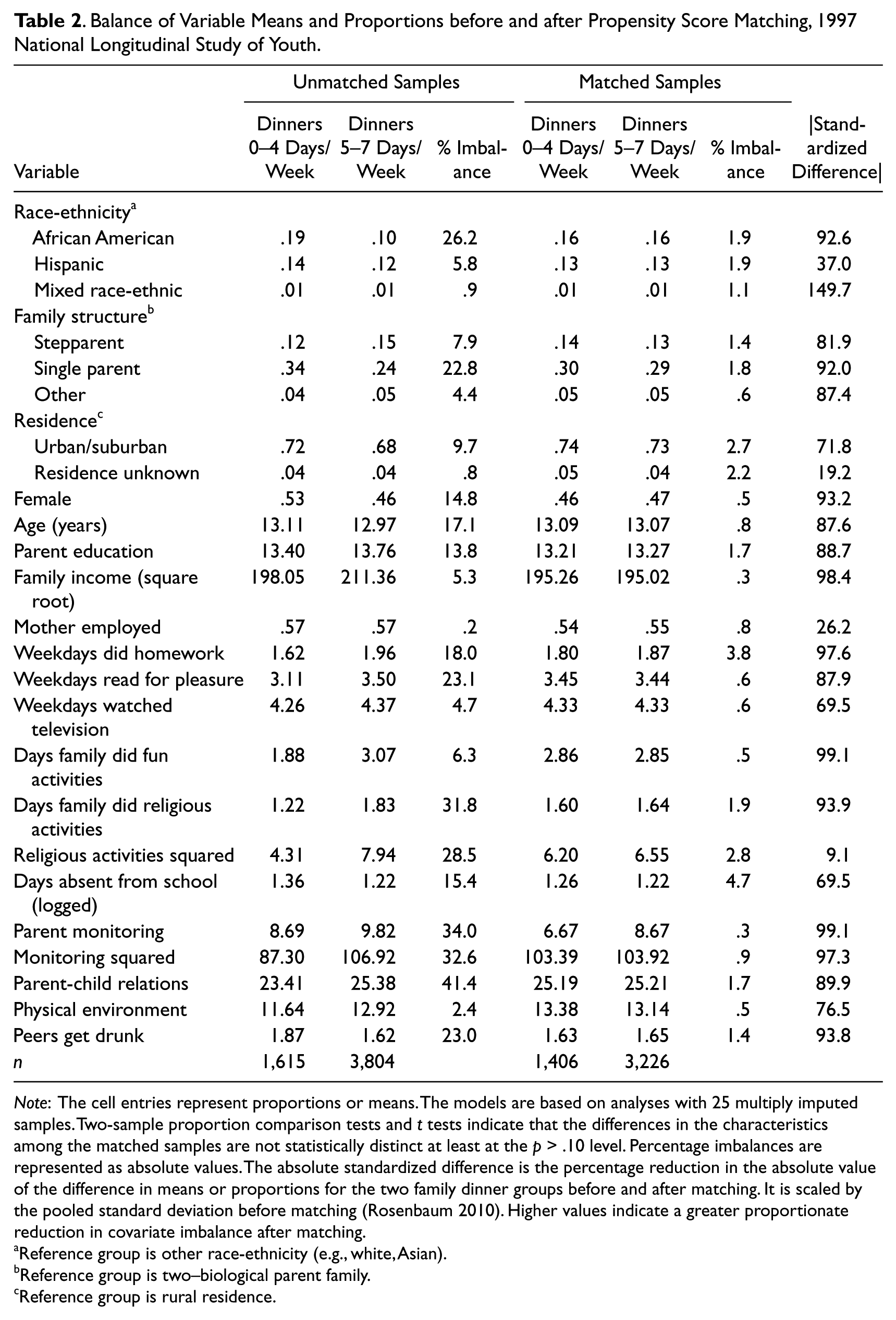
Note: The cell entries represent proportions or means. The models are based on analyses with 25 multiply imputed samples. Two-sample proportion comparison tests and t tests indicate that the differences in the characteristics among the matched samples are not statistically distinct at least at the p > .10 level. Percentage imbalances are represented as absolute values. The absolute standardized difference is the percentage reduction in the absolute value of the difference in means or proportions for the two family dinner groups before and after matching. It is scaled by the pooled standard deviation before matching (Rosenbaum 2010). Higher values indicate a greater proportionate reduction in covariate imbalance after matching.

Reference group is other race-ethnicity (e.g., white, Asian).

Reference group is two–biological parent family.

Reference group is rural residence.

Note that the percentage imbalance prior to matching is up to 41 percent, yet in the matched samples, the percentage imbalance is consistently less than 5 percent. The absolute standardized differences (percentage reduction in bias) show the degree of balancing for each variable (Rosenbaum 2010). Most are quite large. Moreover, two-sample proportion tests and t tests comparing the means indicate that no differences in the matched samples are statistically significant at the p < .10 level. This suggests successful matching for all the covariates.

Table 3 provides the results of the binary and generalized propensity matching models, along with results from the inverse propensity score weighting analyses (Guo and Fraser 2008). The first set of models under each panel shows the difference in substance use prior to matching, or the unadjusted difference. For example, before matching, the difference in the frequency of cigarette smoking is –.129 (p < .001) on a logarithmic scale. Thus, past 30-day cigarette use among those reporting zero to four family dinners per week is expected to be about 12 percent higher than among those reporting five to seven family dinners per week (see the binary treatment panel). Similarly, past 30-day marijuana use among those sharing six or seven family meals is expected to be about 10 percent lower relative to those sharing zero to two family meals (categorical treatment panel). In general, it appears that, prior to matching, family dinners have a modest negative association with alcohol, cigarette, and marijuana use frequency.

Table 3.

Comparison of Effect Sizes of Family Dinners on Adolescent Drug Use, by Type of Propensity Score Adjustment Method, 1997 National Longitudinal Study of Youth

Propensity Score Method	Alcohol Use, Past 30 Days	Cigarette Smoking, Past 30 Days	Marijuana Use, Past 30 Days	Substance Use Initiation vs. Abstention, 1997–1998
Binary treatment (family dinnercoded 0–4 vs. 5–7 days/week)
Unadjusted difference beforematching	−.087***	−.129***	−.074***	−.116
Matched sample group difference	−.018	−.020	−.025	−.065
Categorical treatment (familydinner coded 0–2, 3–5, or 6 or 7 days/week)
Unadjusted difference before propensity weighting^a
Dinners 3 to 5 days/week	−.039*	−.041	−.049**	.291*
Dinners 6 or 7 days/week	−.119***	−.180***	−.101***	.031
Inverse propensity score weighting^a
Dinners 3 to 5 days/week	.015	.026	−.012	−.190
Dinners 6 or 7 days/week	−.022	−.034	−.038*	−.025
Continuous treatment (familydinner coded 0–7 days/week)
Unadjusted model beforematching	−.010	−.011	−.010**	−.004
Generalized propensity scorematching	−.016	−.010	−.014**	−.018

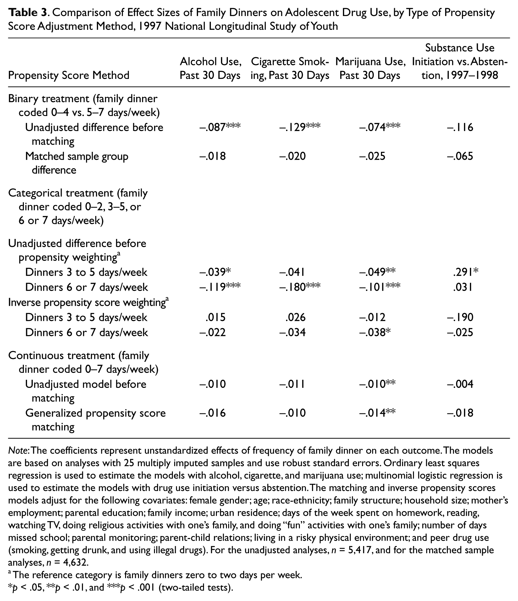
Note: The coefficients represent unstandardized effects of frequency of family dinner on each outcome. The models are based on analyses with 25 multiply imputed samples and use robust standard errors. Ordinary least squares regression is used to estimate the models with alcohol, cigarette, and marijuana use; multinomial logistic regression is used to estimate the models with drug use initiation versus abstention. The matching and inverse propensity scores models adjust for the following covariates: female gender; age; race-ethnicity; family structure; household size; mother’s employment; parental education; family income; urban residence; days of the week spent on homework, reading, watching TV, doing religious activities with one’s family, and doing “fun” activities with one’s family; number of days missed school; parental monitoring; parent-child relations; living in a risky physical environment; and peer drug use (smoking, getting drunk, and using illegal drugs). For the unadjusted analyses, n = 5,417, and for the matched sample analyses, n = 4,632.

The reference category is family dinners zero to two days per week.

p < .05, **p < .01, and ***p < .001 (two-tailed tests).

However, the matched samples analyses indicate that, for most of the comparisons, the association between family dinners and adolescent drug use is due to a selection process and not to any causal influence. For example, in the binary treatment model, the difference in cigarette use diminishes to –.020 (p > .05), whereas the difference in marijuana frequency diminishes to –.025 (p > .05). Note also that none of the family dinner frequency variables affect substance use initiation after matching or weighting.

Nonetheless, matching does not eliminate the association with marijuana use. For instance, those who reported that they share family dinners six or seven days a week manifest a modest decrease (about 4 percent) in marijuana use relative to those who share family dinners zero to two days a week. Moreover, a statistically significant treatment effect on marijuana use remains in the generalized propensity score model, which considers family dinners as continuous. Each one-unit increase in family dinners is associated with about a 2 percent decrease in past 30-day marijuana use (p < .01). We suspect that this result may be due to the threshold effect shown in the categorical model but cannot fully verify if this is the case (see the section on sensitivity analyses for additional information).

Sensitivity Analyses

We conducted several auxiliary analyses to determine whether the results are sensitive to (1) the coding used for family dinners, (2) particular aspects of the propensity score models, (3) possible endogeneity of family dinners, and (4) unobserved factors. First, as mentioned earlier, we varied the measure of family dinners by using different cut points to create alternative binary (e.g., zero to six vs. seven days) and categorical scales. We also evaluated different transformations of the zero-to-seven scale. None of these steps results in different findings in general.

Second, we used different propensity score models by changing the matching algorithm (e.g., different number of matches, matching without replacement, different calipers). We also explored the use of a logistic model for proportions and a boosted regression model to increase the predictive power of the propensity score models (Lee, Lessler, and Stuart 2009). Boosted regression is a data-mining technique that iteratively reweights the regression parameters so that the errors in prediction diminish at each stage until a satisfactory prediction model is obtained (Hastie, Tibshirani, and Friedman 2009, chap. 10). Although it results in an improved prediction model (correct classification increases from 23 percent to 76 percent), it does not achieve sufficient covariate balance.

Third, it is generally recognized that most matching estimators are not consistent when the number of matches is small. Thus, bootstrapped standard errors are often used to attempt to correct this deficiency. According to recent research, however, this approach does not correct for bias (Abadie and Imbens 2008). Thus, we used a bias-corrected matching estimator that is implemented in the Stata package nnmatch to reestimate the binary family dinner models (Abadie and Imbens 2011). A limitation of this package is that it does not provide details about the matching or how it handles the covariates, so we opted to present the models shown earlier. The results of these models reveal that the average treatment effects on the treated are not significantly different from zero, thus supporting the results shown in the first panel of Table 3.

Fourth, to obviate potential endogeneity issues in cross-sectional propensity score models, we reestimated the models using substance use measures at wave 2 as outcome variables. Even the unadjusted difference models using the entire sample do not show a treatment effect; nor do any of the propensity score models. Thus, we do not find support for the effect of family dinners on marijuana use (cf. Table 3, column 4) over a one-year period (1997 to 1998).

Fifth, because the earlier analyses use family dinners measured at the same time as the covariates (1997), there may be reverse causality that is not considered (e.g., family dinners may affect parent-child relations). To guard against this, we estimated a set of models using family dinner frequency during wave 2 (1998) as the treatment indicator. Family dinner frequency and the covariates measured during wave 1 (1997) were used in the prediction equation. The resulting propensity score models showed no statistical relationship with adolescent substance use during wave 2. Once again, even the effects on marijuana use were not confirmed in this model.

Finally, following recent studies (e.g., Miller et al. 2010), we estimated fixed-effects regression models to predict substance use from 1997 to 1998. The fixed-effects model is represented as

Y_{i t} = β_{0} + β_{1} {(family dinners)}_{i t} + β_{q} X_{i t} + u_{i} + ε_{i t},

where X represents the time-varying explanatory variables and u_i is a respondent-specific term, or the fixed effect. Family dinners is denoted it, which indicates that it is allowed to change across the two waves. The fixed-effect represents observed and unobserved characteristics of respondents. The ϵ_it term indicates random noise that exists within and across units but may also include the effects of omitted variables. Because within-respondent variation is used to estimate the effects in this model, there tends to be reduced bias in coefficients designed to predict adolescent drug use (Frees 2004). Unfortunately, in addition to substance use and family dinners, the number of time-varying explanatory factors is limited to parent-child relations, parental monitoring, mother’s employment, family income, and two time use variables (family does something fun or does something religious together). Thus, the models are underfit.

The results of the fixed-effects models suggest that the continuous measure of family dinners has a modest longitudinal impact on alcohol, cigarette, and marijuana use (e.g., β[alcohol use] = –.004, p ≈ .03; cf. Musick and Meier 2012) but no discernible effect on substance use initiation. Nevertheless, a key assumption is that the treatment variable is not correlated with unobserved characteristics housed in ϵ_it. If this assumption is not met, then the fixed-effects models will provide biased results. Moreover, as mentioned earlier, studies indicate that fixed-effects estimators yield substantial bias and are relatively inefficient for capturing causal effects (Dehejia and Wahba 1999; Michalopoulos et al. 2004). Thus, propensity score matching is the recommended alternative.

Discussion

Research indicates that early adolescent substance use is associated with negative outcomes such as delinquent and criminal behavior, attenuated educational achievement, and impaired emotional and physical health (e.g., Hall and Degenhardt 2009; Krohn et al. 1997). It is therefore not surprising that numerous programs have been designed to prevent adolescent substance use. And, given the expense and complexities of many of these programs, some experts hope to find relatively simple methods of prevention.

These methods often include programs that warn about the health risks of substance use. Yet most such efforts have been ineffective. Rather than concluding that simple solutions are unproductive, however, experts continue to search for a prevention keystone that is both effectual and can be manipulated via public policy campaigns. Perhaps none has garnered as much attention in recent years as family meals. Promoted by policy experts and scholars alike (e.g., Califano 2007; Fiese and Schwartz 2008), shared family meals are seen as an excellent opportunity for parents to positively influence child development. As noted in a white paper released by the National Center on Addiction and Substance Abuse,

Parental engagement fostered around the dinner table is one of the most potent tools to help parents raise healthy, drug-free children. . . . We know from years of research that teens whose parents are “hands on”—engaged in their teens’ day to day lives, relaxing with them, having frequent family dinners, supervising them, establishing standards of behavior, and setting positive examples of healthy behavior—are much less likely to use drugs, drink or smoke. (2012:i–ii)

As this statement suggests, though, it is not family meals themselves that prevent substance use but rather characteristics of the surrounding family environment that affect both engagement during family dinners and substance use. Recent research using national data sets supports this notion, for once controls for family factors are considered, the impact of shared dinners on substance use and other problem behaviors is attenuated (Miller et al. 2012; Musick and Meier 2012; see, however, Sen 2010).

In this study, we take an alternative approach, one that moves us closer to identifying whether family dinners have a causal impact on substance use, by using propensity scores to create matched “treatment” and “control” groups (Dehejia and Wahba 2002; Rosenbaum 2010). Moreover, because there is no standard way of measuring the frequency of family dinners (cf. Fulkerson et al. 2006; Sen 2010), we estimate their effects using three distinct measurement strategies. The results of our analysis cast doubt on the notion that family dinners, in isolation from other family characteristics, offer general protection against either substance use initiation or the frequency with which illicit substances are used. We find that, after matching and regression adjustment, the frequency of family dinners does not affect alcohol or cigarette use; nor is it associated with substance use initiation. It is important to note that experts argue that preventing initiation is particularly vital among young adolescents, because early onset portends problems with substances and other health issues later in life (Kosterman et al. 2000). Thus, the lack of an association with family dinners is a key finding.

However, in two instances, family dinners do affect marijuana use. Even after matching and regression adjustment, there is less marijuana use among adolescents who report more frequent family dinners when they are measured categorically or continuously. It is not clear why the effect on marijuana use differs from the effect on alcohol and cigarette use, but it may have to do with the strict illegal status of marijuana. Although alcohol and tobacco use are illegal for adolescents, they are used more often and are more widely available to youth in the United States. Thus, family dinners may be more consequential for behaviors that are clearly illicit or outside the bounds of normative family behaviors.

Given these general findings, though, it seems that the most important approach to understanding the causes of early adolescent drug use is to address the broader family environment, rather than focusing on family dinners in isolation from other conditions. Family environments include how well parents and adolescents get along, communicate, and identify with one another (e.g., Bahr et al. 2005; Franko et al. 2008). Studies might still consider family meals as an indicator of family interaction, but attempting to isolate their effects on adolescent behaviors seems shortsighted. Yet it remains important to consider the association between family meals and marijuana use, because the findings suggest a modest causal impact that is not accounted for by other factors (cf. Eisenberg et al. 2008; Musick and Meier 2012).

Moreover, it is vital for research to consider the broader contextual factors that likely influence family meals, family relations, and substance use. For example, in communities marked by high levels of joblessness and poverty, low social cohesion, and dilapidated housing, parenting is especially difficult and may therefore affect disruptions in family routines and lead to more problem behaviors (Hoffmann 2002; McLeod and Nonnemaker 2000). Thus, future research on the family environment and adolescent substance use should attend to broader contextual factors that may confound, magnify, or otherwise account for their complex associations.

Limitations

Although we have undertaken a relatively comprehensive analysis, there are several limitations that point to the need for additional research. First, the models may violate the unconfoundedness assumption (Rosenbaum 2010), which notes that the treatment indicator should be independent of the potential outcomes conditional on pretreatment variables. This means that all variables that affect both the outcome and the likelihood of receiving treatment are observed. Yet there are bound to be unobserved covariates that we could not examine. For example, genetic factors may affect the association between family dinners and substance use (Daw et al. 2013; Guo, Roettger, and Cai 2008).

Second, although we consider this issue in the sensitivity analyses, we cannot fully determine whether the covariates precede the treatment. Moreover, it is possible that family dinners and other variables, including the outcomes, are related reciprocally (White and Halliwell 2011). This has implications for attempts to estimate the probability or the distribution of family dinners and how they relate to adolescent behaviors. For example, youth who already use, say, marijuana may subsequently withdraw from family activities, including family dinners. And it may be this withdrawal process that leads to greater involvement in marijuana use rather than any effect of shared family meals or other aspects of family life. Future research should explore these associations in detail.

Third, there may be reporting bias when it comes to substance use and some of the explanatory variables, even though self-administered response cards were used in the NLSY97. Systematic underreporting of substance use is a problem in most large-scale surveys (Shillington and Clapp 2000). The degree of bias is unknown, however, so alternative models are needed that correct for unobserved biases.

Conclusion

In summary, we find scant evidence that the frequency of family dinners has a general causal impact on adolescent substance use. Although previous research and position papers from influential advocates contend that sharing family meals is a significant way to prevent adolescents from using illicit substances, the results of the present analysis cast doubt on such a broad assertion. Rather, as suggested by recent studies, there are likely other factors—some of which are related to the family environment, but may also include genetic influences, personality traits, and social or cultural contexts—that influence the risks of adolescent substance use and account for any effectiveness of family meals. Nevertheless, family meals appear to have a modest causal effect on the frequency of marijuana use, a finding that calls for additional research on whether family meals can offer a short-term preventive measure to an important form of adolescent substance use. In summary, though, future studies should examine not only the selection process that affects family dinners but also whether family meals are part of a broader set of conditions that lead adolescents toward or away from engaging in substance use and other risky behaviors.

Footnotes

Acknowledgements

We appreciate the advice and assistance provided by Lance Erickson, Steve Bahr, Marco Steenbergen, Dominik Hangartner, Debra Umberson, and several anonymous reviewers.

Author Biographies

John P. Hoffmann is a professor in the Department of Sociology at Brigham Young University and in the Department of Criminology and Criminal Justice at the University of South Carolina. His recent research has appeared in the Journal of Studies on Alcohol and Drugs, Social Forces, and Criminology. His research interests include the etiology of delinquency and drug use.

Elizabeth Warnick recently completed an MS degree in sociology from Brigham Young University. Her research focuses on educational effects on social stratification.

References

Abadie

Alberto

Imbens

Guido W.

2008. “On the Failure of the Bootstrap for Matching Estimators.” Econometrica 76(6):1537–57.

Abadie

Alberto

Imbens

Guido W.

2011. “Bias-corrected Matching Estimators for Average Treatment Effects.” Journal of Business & Economic Statistics 29(1):1-11.

Allen

Mike

Donohue

William A.

Griffin

Amy

Ryan

Dan

Mitchell Turner

Monique M.

2003. “Comparing the Influence of Parents and Peers on the Choice to Use Drugs: A Meta-analytic Summary of the Literature.” Criminal Justice and Behavior 30(2):163-86.

Aughinbaugh

Alison

Gardecki

Rosella M.

2007. Attrition in the National Longitudinal Survey of Youth 1997. Columbus, OH: Center for Human Resource Research.

Bahr

Stephen J.

Hoffmann

John P.

Yang

Xiaoyan

. 2005. “Parental and Peer Influences on the Risk of Adolescent Drug Use.” Journal of Primary Prevention 26(6):529–51.

Bailey

Susan L.

Hubbard

Robert L.

1990. “Developmental Variation in the Context of Marijuana Initiation among Adolescents.” Journal of Health and Social Behavior 31(1):58–70.

Brook

Judith S.

Brook

David W.

Richter

Linda

Whiteman

Martin

. 2006. “Risk and Protective Factors of Adolescent Drug Use: Implications for Prevention Programs.” Pp. 265–87 in Handbook of Drug Abuse Prevention, edited by Sloboda

Bukoski

W. J.

New York: Springer.

Califano

Joseph A.

2007. High Society: How Substance Abuse Ravages America and What to Do About It. New York: Public Affairs.

Catalano

Richard F.

Kosterman

Rick

Hawkins

J. David

Newcomb

Michael D.

Abbott

Robert D.

1996. “Modeling the Etiology of Adolescent Substance Use: A Test of the Social Development Model.” Journal of Drug Issues 26(2):429–55.

10.

Center for Human Resource Research. 2004. NLSY97 User’s Guide: A Guide to the Rounds 1–4 Data National Longitudinal Survey of Youth 1997. Columbus, OH: Center for Human Resource Research.

11.

Center for Human Resource Research and Child Trends. 1999. Appendix 9: Family Process and Adolescent Outcome Measures. Columbus, OH: Center for Human Resource Research.

12.

Davidson

Rebecca

Gauthier

Anne H.

2010. “A Cross-national Multi-level Study of Family Meals.” International Journal of Comparative Sociology 51(5):349–65.

13.

Daw

Jonathan

Shanahan

Michael

Harris

Kathleen Mullan

Smolen

Andrew

Haberstick

Brett

Boardman

Jason D.

2013. “Genetic Sensitivity to Peer Behaviors: 5HTTLPR, Smoking, and Alcohol Consumption.” Journal of Health and Social Behavior 54(1):92–108.

14.

Dehejia

Rajeev H.

Wahba

Sadek

. 1999. “Causal Effects in Nonexperimental Studies.” Journal of the American Statistical Association 94(448):1053–62.

15.

Dehejia

Rajeev H.

Wahba

Sadek

. 2002. “Propensity Score Matching Methods for Nonexperimental Causal Studies.” Review of Economics and Statistics 84(1):151–61.

16.

Eisenberg

Marla E.

Neumark-Sztainer

Dianne

Fulkerson

Jayne A.

Story

Mary

. 2008. “Family Meals and Substance Use: Is There a Long-term Protective Association?” Journal of Adolescent Health 43(2):151–56.

17.

Ellickson

Phyllis L.

McCaffrey

Daniel F.

Ghosh-Dastidar

Bonnie

Longshore

Douglas L.

2003. “New Inroads in Preventing Adolescent Drug Use: Results from a Large-scale Trial of Project ALERT in Middle Schools.” American Journal of Public Health 93(11):1830–36.

18.

Ennett

Susan T.

Ringwalt

Christopher L.

Thorne

Judy

Rohrbach

Louise Ann

Vincus

Amy

Simons-Rudolph

Ashley

Jones

Shelton

. 2003. “A Comparison of Current Practice in School-based Substance Use Prevention Programs with Meta-analysis Findings.” Prevention Science 4(1):1–14.

19.

Fiese

Barbara H.

Foley

Kimberly P.

Spagnola

Mary

. 2006. “Routine and Ritual Elements in Family Mealtimes: Contexts for Child Wellbeing and Family Identity.” New Directions for Child and Adolescent Development 2006(111):67–90.

20.

Fiese

Barbara H.

Schwartz

Marlene

. 2008. “Reclaiming the Family Table: Mealtimes and Child Health and Wellbeing.” Social Policy Report 22(4):3–18.

21.

Franko

Debra L.

Thompson

Douglas

Affenito

Sandra G.

Barton

Bruce A.

2008. “What Mediates the Relationship Between Family Meals and Adolescent Health Issues?” Health Psychology 27(2):S109–17.

22.

Frees

Edward W.

2004. Longitudinal and Panel Data. New York: Cambridge University Press.

23.

Fulkerson

Jayne A.

Story

Mary

Mellin

Alison

Leffert

Nancy

Neumark-Sztainer

Dianne

French

Simone A.

2006. “Family Dinner Meal Frequency and Adolescent Development: Relationships with Developmental Assets and High-risk Behaviors.” Journal of Adolescent Health 39(3):337–45.

24.

Green

Brian E.

Ritter

Christian

. 2000. “Marijuana Use and Depression.” Journal of Health and Social Behavior 41(1):40–9.

25.

Griffin

Kenneth W.

Botvin

Gilbert J.

Scheier

Lawrence M.

Diaz

Tracy

Miller

Nicole L.

2000. “Parenting Practices as Predictors of Substance Use, Delinquency, and Aggression among Urban Minority Youth: Moderating Effects of Family Structure and Gender.” Psychology of Addictive Behaviors 14(2):174–84.

26.

Guo

Guang

Roettger

Michael E.

Cai

Tianji

. 2008. “The Integration of Genetic Propensities into Social-control Models of Delinquency and Violence among Male Youths.” American Sociological Review 73(4):543–68.

27.

Guo

Shenyang

Fraser

Mark W.

2010. Propensity Score Analysis: Statistical Methods and Applications. Thousand Oaks, CA: Sage.

28.

Hair

Elizabeth C.

Anderson Moore

Kristin

Garrett

Sarah B.

Ling

Thomson

Cleveland

Kevin

. 2008. “The Continued Importance of Quality Parent-adolescent Relationships during Late Adolescence.” Journal of Research on Adolescence 18(1):187–200.

29.

Hall

Wayne

Degenhardt

Louisa

. 2009. “Adverse Health Effects of Non-medical Cannabis Use.” Lancet 374(9698):1383–91.

30.

Hastie

Trevor

Tibshirani

Robert

Friedman

Jerome

. 2009. The Elements of Statistical Learning. New York: Springer.

31.

Hirano

Keisuke

Imbens

Guido W.

2004. “The Propensity Score with Continuous Treatments.” Pp.73–84 in Applied Bayesian Modeling and Causal Inference from Incomplete-Data Perspectives, edited by Gelman

Meng

X. L.

New York: Wiley InterScience.

32.

Hoffmann

John P.

2002. “The Community Context of Family Structure and Adolescent Drug Use.” Journal of Marriage and Family 64(2):314–30.

33.

Hornik

Robert

Jacobsohn

Lela

Orwin

Robert

Piesse

Andrea

Kalton

Graham

. 2008. “Effects of the National Youth Anti-drug Media Campaign on Youths.” American Journal of Public Health 98(12):2229–36.

34.

Kosterman

Rick

Hawkins

J. David

Guo

Jie

Catalano

Richard F.

Abbott

Robert D.

2000. “The Dynamics of Alcohol and Marijuana Initiation: Patterns and Predictors of First Use in Adolescence.” American Journal of Public Health 90(3):360–66.

35.

Krohn

Marvin D.

Lizotte

Alan J.

Perez

Cynthia M.

1997. “The Interrelationship between Substance Use and Precocious Transitions to Adult Statuses.” Journal of Health and Social Behavior 38(1):87–103.

36.

Lee

Brian

Lessler

Justin

Stuart

Elizabeth A.

2009. “Improving Propensity Score Weighting Using Machine Learning.” Statistics in Medicine 29(3):337–46.

37.

Macleod

John

Oakes

Rachel

Copello

Alex

Crome

Ilana

Egger

Matthias

Hickman

Mathew

Oppenkowski

Thomas

Stokes-Lampard

Helen

Smith

George Davey

. 2004. “Psychological and Social Sequelae of Cannabis and Other Illicit Drug Use by Young People: A Systematic Review of Longitudinal, General Population Studies.” Lancet 363(9421):1579–88.

38.

McLeod

Jane D.

Nonnemaker

James M.

2000. “Poverty and Child Emotional and Behavioral Problems: Racial/Ethnic Differences in Processes and Effects.” Journal of Health and Social Behavior 41(2):137–61.

39.

Michalopoulos

Charles

Bloom

Howard S.

Hill

Carolyn J.

2004. “Can Propensity Score Methods Match the Findings from a Random Assignment Evaluation of Mandatory Welfare-to-work Programs?” Review of Economics and Statistics 86(1):156–79.

40.

Miller

Daniel P.

Waldfogel

Jane

Han

Wen-Jui

. 2012. “Family Meals and Child Academic and Behavioral Outcomes.” Child Development 83(6):2104–20.

41.

Morgan

Stephen L.

Harding

David J.

2006. “Matching Estimators of Causal Effects: Prospects and Pitfalls in Theory and Practice.” Sociological Methods & Research 35(1):3–60.

42.

Musick

Kelly

Meier

Ann

. 2012. “Assessing Causality and Persistence in Associations between Family Dinners and Adolescent Well-being.” Journal of Marriage and Family 74(3):476–93.

43.

Nargiso

Jessica E.

Friend

Karen

Florin

Paul

. Forthcoming. “An Examination of Peer, Family, and Community Context Risk Factors for Alcohol Use and Alcohol Use Intentions in Early Adolescents.” Journal of Early Adolescence.

44.

National Center on Addiction and Substance Abuse. 2012. The Importance of Family Dinners VIII. New York: National Center on Addiction and Substance Abuse.

45.

Repetti

Rena L.

Taylor

Shelley E.

Seeman

Teresa

. 2002. “Risky Families: Family Social Environments and the Mental and Physical Health of Offspring.” Psychological Bulletin 128(2):330–66.

46.

Rosenbaum

Paul R.

2010. Design of Observational Studies. New York: Springer.

47.

Rosenbaum

Paul R.

Rubin

Donald B.

1983. “The Central Role of the Propensity Score in Observational Studies for Causal Effects.” Biometrika 70(1):41–55.

48.

Rubin

Donald B.

Thomas

Neal

. 2000. “Combining Propensity Score Matching with Additional Adjustments for Prognostic Covariates.” Journal of the American Statistical Association 95(450):573–85.

49.

Sen

Bisakha

. 2010. “The Relationship between Frequency of Family Dinner and Adolescent Problem Behaviors after Adjusting for Other Family Characteristics.” Journal of Adolescence 33(1):187–96.

50.

Shillington

A. M.

Clapp

J. D.

2000. “Self-report Stability of Adolescent Substance Use: Are There Differences for Gender, Ethnicity and Age?” Drug and Alcohol Dependence 60(1):19–27.

51.

Slade

Eric P.

Stuart

Elizabeth A.

Salkever

David S.

Karakus

Mustafa

Green

Kerry M.

Ialongob

Nicholas

. 2008. “Impacts of Age of Onset of Substance Use Disorders on Risk of Adult Incarceration among Disadvantaged Urban Youth: A Propensity Score Matching Approach.” Drug and Alcohol Dependence 95(1–2):1–13.

52.

Stuart

Elizabeth A.

2010. “Matching Methods for Causal Inference: A Review.” Statistical Science 25(1):1–21.

53.

Tepper

Robin L.

2001. “Parental Regulation and Adolescent Discretionary Time-use Decisions: Findings from the NLSY97.” Pp.79–105 in Social Awakening: Adolescent Behavior as Adulthood Approaches, edited by Michael

R. T.

New York: Russell Sage.

54.

Van Buuren

Brand

J.P.L.

Groothuis-Oudshoorn

C.G.M.

Rubin

D.B.

2006. “Fully Conditional Specification in Multivariate Imputation.” Journal of Statistical Computation and Simulation 76(12):1049–64.

55.

von Hippel

Paul

. 2007. “Regression with Missing Ys: An Improved Strategy for Analyzing Multiply Imputed Data.” Sociological Methodology 37(1):83–117.

56.

White

James

Halliwell

Emma

. 2010. “Alcohol and Tobacco Use during Adolescence: The Importance of the Family Mealtime Environment.” Journal of Health Psychology 15(4):526–32.

57.

White

James

Halliwell

Emma

. 2011. “Family Meal Frequency and Alcohol and Tobacco Use in Adolescence: Testing Reciprocal Effects.” Journal of Early Adolescence 31(5):735–49.

58.

Wiesner

Margit

Kim

Hyoun K.

Capaldi

Deborah M.

2005. “Developmental Trajectories of Offending: Validation and Prediction to Young Adult Alcohol Use, Drug Use, and Depressive Symptoms.” Development and Psychopathology 17(1):251–70.