Color segmentation of multi-colored fabrics using self-organizing-map based clustering algorithm

Abstract

Fabric prints may contain intricate and nesting color patterns. To evaluate colors on such a fabric, regions of different colors must be measured individually. Therefore, precise separation of colored patterns is paramount in analyzing fabric colors for digital printing, and in assessing the colorfastness of a printed fabric after a laundering or abrasion process. This paper presents a self-organizing-map (SOM) based clustering algorithm used to automatically classify colors on printed fabrics and to accurately partition the regions of different colors for color measurement. The main color categories of an image are firstly identified and flagged using the SOM’s density map and U-matrix. Then, the region of each color category is located by divining the U-matrix map with an adaptive threshold, which is determined by recursively decreasing it from a high threshold until all the flagged neurons are assigned to different regions in the divided map. Finally, the regions with high color similarity are merged to avoid possible over-segmentation. Unlike many other clustering algorithms, this algorithm does not need to pre-define the number of clusters (e.g. main colors) and can automatically select a distance threshold to partition the U-matrix map. The experimental results show that the intricate color patterns can be precisely separated into individual regions representing different colors.

Keywords

multi-colored fabric self-organizing map clustering color segmentation

The serviceability of a printed fabric is dictated by its colorfastness performance, which is often evaluated by comparing colors on the fabric before and after a laundering or abrasion test.^1,2 For a solid-color fabric, color measurement can be performed randomly on the fabric surface. For a fabric that contains multiple colors and intricate patterns, colorfastness evaluation must be performed separately on regions with distinctive colors.³ The regions corresponding to colored patterns need to be partitioned based on their unique color characteristics so that the statistics of color values for each region can be calculated independently.

In order to partition colored patterns in a fabric image, the number of colors in the image must be identified, and the boundaries of each color region must be defined. Unlike other materials, a fabric often has an appearance where colored regions do not have clearly defined boundaries. Thus, only soft clustering algorithms are suitable for this specific application. K-means and fuzzy c-means (FCM) are the two widely used clustering methods,^4,5 and have been applied for color segmentation.^6–8 However, these two methods require the number of clusters to be pre-defined prior to the implementation, which makes them inapplicable to segmenting complex color patterns. Luo et al.⁹ developed a probabilistic model specifically for dissecting yarns in a yarn-dyed fabric image.

The self-organizing map (SOM) is an unsupervised neural-network technique that can identify the number of clusters because of its visualization property.¹⁰ Many papers have presented methods to detect the number of clusters by finding contiguous regions on the SOM’s unified distance matrix (U-matrix), a representation where the Euclidean distances between neighboring neurons are depicted in a grayscale image, but have not explained how to determine the precise borders of detected clusters.^11–18 To attain a fine segmentation of a printed color pattern, researchers have designed hybrid methods combining the SOM and other clustering algorithms for automatic identification of both color categories and regions.^3,19

In this study, we proposed a SOM-based algorithm for automatic color identification and clustering that can precisely partition colored regions to enable the colorfastness evaluation for printed fabrics. This color-clustering algorithm is solely based on the SOM’s density map and U-matrix, and takes three steps: coarse partition, cluster refinement and cluster merging. In the coarse partition, neurons associated with the main colors are identified and flagged separately. In the cluster refinement, the optimal distance threshold is adaptively selected to divide the U-matrix into regions (clusters) that correspond to different color categories. The distance threshold is determined by continuously decreasing the threshold from a high initial value to a number when all the flagged neurons are assigned to different regions in the divided map. In the cluster-merging stage, clusters with similar color characteristics are merged to avoid over-segmentation.

Self-organizing map

In early the 1980s, the SOM was invented by Kohonen¹⁰ to map a set of p-dimensional vectors to a low-dimensional, typically two-dimensional (2D), topographic map. Figure 1 shows a typical SOM network that consists of an input layer and an output layer. The input layer represents a set of input vectors. The output layer contains a number of neurons arranged on a hexagonal or rectangular grid. The neurons in the output layer are fully connected to the units in the input layer with different weight vectors.

Figure 1.

The self-organizing map network.

The input data set X = {x₁, x₂,…, x_N} is a subset of $R^{p}$ , where p is the dimension of input vectors. Let i denote the ith neuron in the output layer, and $w i (w i = [w i 1, w i 2, \dots, w ip])$ the weight vector of neuron i. At time t in the training process, for one input vector x_j, neuron b in the output layer is the winner or the best matching unit (BMU) if

‖ x j - w b ‖ = min {‖ x j - w i ‖}, i = 1, 2, 3, \dots, M

(1)

where

‖ \cdot ‖

is a distance measurement and M is the number of neurons in the output layer. Then, the weight vectors of the winner neuron, b, and its neighboring neurons are modified using the following update rule

w k (t + 1) = {w k (t) + a (t) [x j - w k (t)], k \in N b (t) w k (t), k \notin N b (t)

(2)

where N_b(t) denotes the set of neighboring neurons of b at time t and a is a learning coefficient. N_b(t) is a function of time t

N b (t) = exp (- \frac{d_{bk}^{2}}{2 r^{2} (t)})

(3)

where d_b_k is the distance between neurons b and k and r is a decreasing function of t. As a result of such training, the vectors that are close to each other in the input space will be mapped onto one neuron or neighboring neurons in the output layer.

U-matrix map

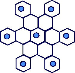
The SOM’s U-matrix map provides a visualization of distances between neighboring neurons on the output layer.¹⁰ In a U-matrix map, each output neuron is normally represented by a hexagon in a 2D grid. The distances between a neuron and its neighbors are represented by extra units inserted between adjacent neurons. If the SOM’s output layer has $m \times n$ neurons, the U-matrix then has $(2 \times m - 1) \times (2 \times n - 1)$ units. Figures 2(a) and (b) show a three-color yarn-dyed knitted fabric (image 1) and its U-matrix map, respectively, in which the distance units are marked with grayscale values proportional to distances. Lighter colors represent smaller distances, that is, higher similarity between neighboring neurons. Thus, a group of light-color units can be seen as one cluster, while the dark units resemble the boundaries between clusters. From this U-matrix map (Figure 2(b)), two clusters (light-color regions) may be located by setting a grayscale threshold on the map. In a U-matrix, a neuron may be adjacent to six neighbors, as shown in Figure 3, in which black dots represent neurons and hexagons represent distance units.

Figure 2.

(a) Sample fabric image (image 1) and (b) U-matrix map.

Figure 3.

Adjacent neurons in the U-matrix.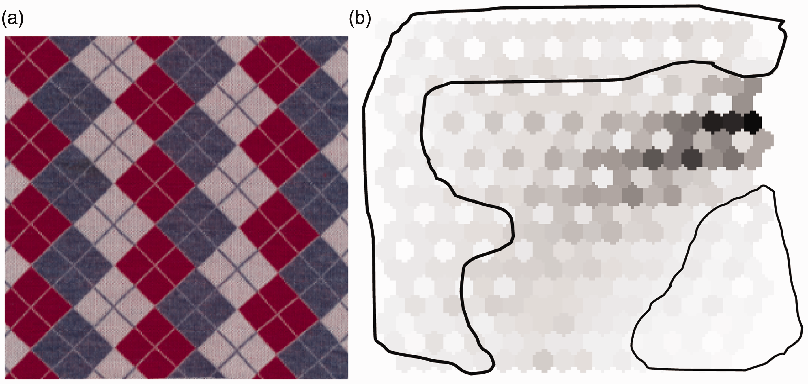

Density map

The cluster structure of a SOM can be also displayed by its density map, which shows the number of hits of each neuron. After the SOM training, each input vector has one BMU. The number of hits on an output neuron is the number of input vectors whose BMU is this neuron. The neurons with few (even zero) hits can be seen as the borders of clusters. This information can be used to design clustering algorithms.^3,17,18 Figure 4(a) shows the density map of the fabric image in Figure 2(a). The number of hits of each neuron is indicated by the size of a green hexagon. Small hexagons indicate low hits and the corresponding neuron can be considered as the separations among clusters. By selecting a proper threshold on hits, this density map can be split into two clusters (the circled regions in Figure 4(a)). Figure 4(b) is a combined map, which superimposes the U-matrix (distance) map and the density (hit) map. By utilizing both distance and density information from a trained SOM, one can achieve more realistic segmentation.¹⁸

Figure 4.

(a) Density map and (b) superimposed map.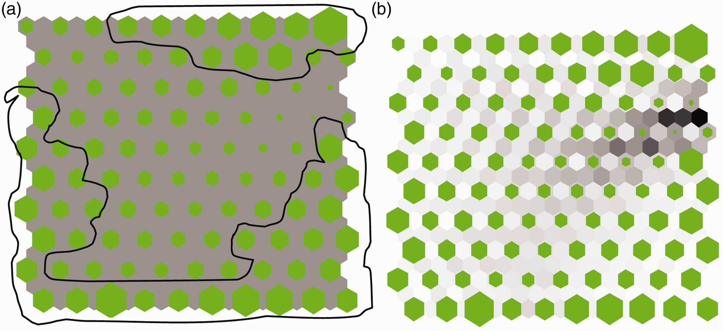

SOM-based clustering algorithm

In this application, the fabric images were captured with a digital scanner and were stored in 24-bit bitmaps in the red, green, blue (RGB) color format. The RGB color space was then transferred into the CIE Lab color space.²⁰ The input vectors of the SOM are the color coordinates (CIE Lab) of all the pixels in a color fabric image. Given a K-pixel image, the SOM has K input vectors, x_j = (L_j, a_j, b_j) (j = 1, 2, … , K). The output layer of the SOM is a map of 10 × 10 neurons. The SOM algorithm consisted of three steps: coarse partition, cluster refinement and cluster merging, and was implemented in Mathworks MATLAB and the SOM toolbox.²¹

Coarse partition

The coarse partition is a step to find out the main clusters (the clusters with a large number of pixels) in an image. The neurons with low hit counts in a density map can be seen as the borders of different clusters. In a density map, a region of connected neurons that have high hits represents one main cluster. Such a region can be seen as a hill in the map, and the neuron with the most hits in the region can be seen as the hill top. The number of hill tops is the number of main colors in an image. In the corresponding U-matrix, a main cluster is a region containing neurons with small distances between each other, and the neuron with the most hits is considered as a hill top since it is the largest contributor to the formation of the cluster during the process of SOM training. If a neuron is selected as a hill top both from the density map and the U-matrix, it should be counted as a main cluster.

Assume that the size of the output layer of a SOM is $m \times n$ . Let w_h(i, j) denote the number of hits of neuron o(i, j) (1 ≤ I ≤ m, 1 ≤ j ≤ n), and a_h denote the average hits of all the w_h. A binary matrix, h(i,j), can be obtained simply by thresholding w_h with a_h

h (i, j) = {0, if w h (i, j) < a h 1, if w h (i, j) \geq a h

(4)

In h(i, j), a region of ‘1’ in the four-connection mode can be regarded as a cluster, and different clusters can be labeled alphabetically (see Figure 5). Binary matrix t₁ is created to indicate the hill tops on the density map (see Figure 6).

Figure 5.

Regions in the h matrix showing coarse segmentation in the density map of image 1 in Figure 2(a). Letters label different regions.

Figure 6.

Matrix t₁, showing the hill tops in the density map of image 1.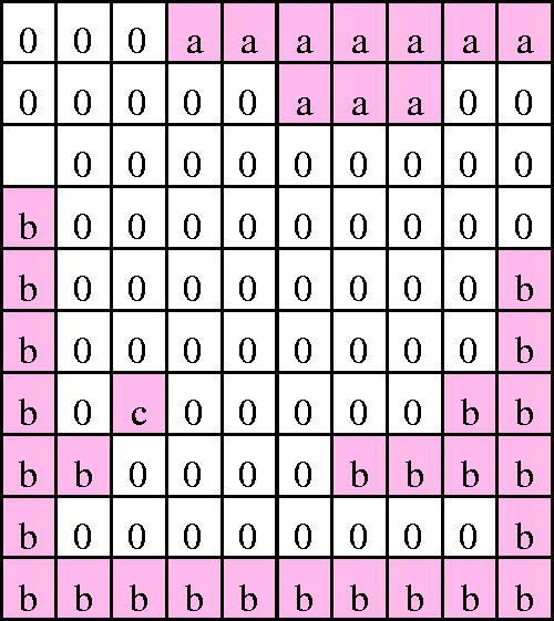

Similarly, the hill tops on the U-matrix map can be obtained through the binary operations. Let w_d(i, j) represent the average of the distances between neuron o(i, j) and its neighbors. According to the definition of the U-matrix, w_d(i, j) can be extracted from the U-matrix, U(k, l), as follows

for i = 1 to m for j = 1 to n k = 2 * I - 1 l = 2 * j - 1 w d (i, j) = U (k, l) endfor endfor

From w_h(i, j) and w_d(i, j), a new matrix can be calculated as w_r(i, j) = w_h(i, j) / w_d(i, j). Let a_r denote the average of all the elements in w_r(i, j), (1 ≤ I ≤ m, 1 ≤ j ≤ n). The binary matrix, s(i,j), can be attained by thresholding w_r with a_r

s (i, j) = {0, if w r (i, j) < a r 1, if w r (i, j) \geq a r

(5)

Figure 7 shows the three labeled ‘1’ regions (four-connection) in s(i,j). The ‘0’ regions represent coarse borders separating the ‘1’ regions. Another binary matrix, t₂, is used to indicate the hill tops (with the most hits) of the labeled regions (see Figure 8).

Figure 7.

Labeled regions in matrix s, showing coarse segmentation in the w_r of image 1. Each region is labeled as a letter.

Figure 8.

Matrix t₂, showing the hill tops in the w_r of image 1.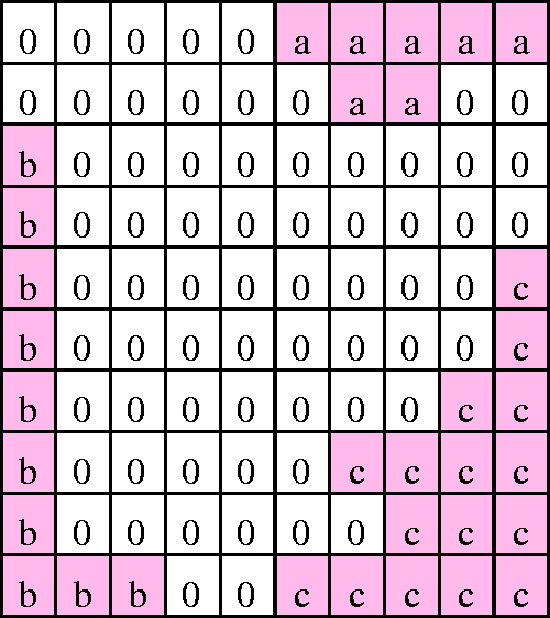

A new flag matrix can be achieved via the AND operation on t₁ and t₂, that is,

F (i, j) = t 1 (i, j) \times t 2 (i, j)

The neurons labeled as ‘1’ in matrix F(i, j) are called flagged neurons, which represent the minimal number of clusters after the coarse partition. Figure 9 displays the two flagged neurons in the SOM of image 1, meaning that this fabric has at least two dominant colors.

Figure 9.

Matrix F for showing the flagged neurons in the self-organizing map of image 1.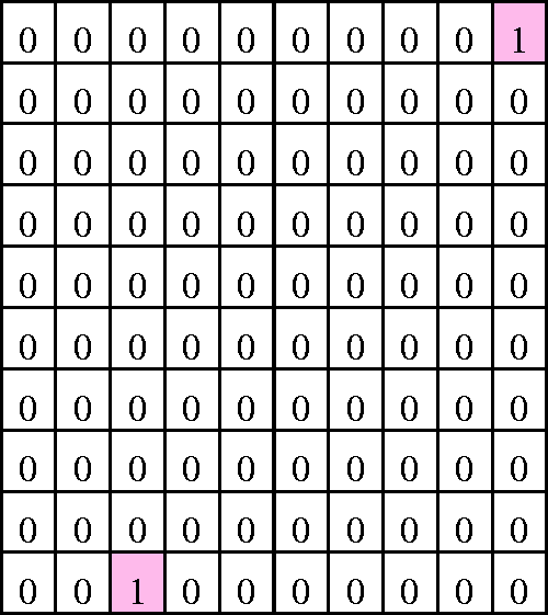

The number of flagged neurons shows the minimal number of main colors present in an image. There may be other main colors (clusters) that are not flagged in the matrix. According to the definition of w_r and s, a neuron o(i, j) with a large number of hits and a large distance may be seen as a border (a ‘0’ element) in matrix s when $\frac{w h (i, j)}{w d (i, j)} < a r$ , that is, o(i,j) cannot be a flagged neuron when its average of distances, w_d(i, j), is larger than $\frac{w h (i, j)}{a r}$ . Missing clusters will be re-sought in the process of cluster refinement.

Figures 10(a)–(h) show another example of a printed multi-color fabric image (image 2), the U-matrix, the density map and the matrixes used for the coarse cluster segmentation. Matrix F indicated that there are four major colors found in image 2 (Figure 10(h)). Because of its intricate color patterns, the main colors in image 2 would be difficult to distinguish manually.

Figure 10.

(a) Sample fabric image (image 2). (b). U-matrix map. (c). Density map. (d). Labeled regions in the h matrix (coarse segmentation in the density map). (e). Matrix t₁ (the hill tops in the density map). (f). Labeled regions in matrix s (coarse segmentation in w_r). (g). Matrix t₂ (the hill tops in w_r). (h). Matrix F (the flagged neurons—main clusters).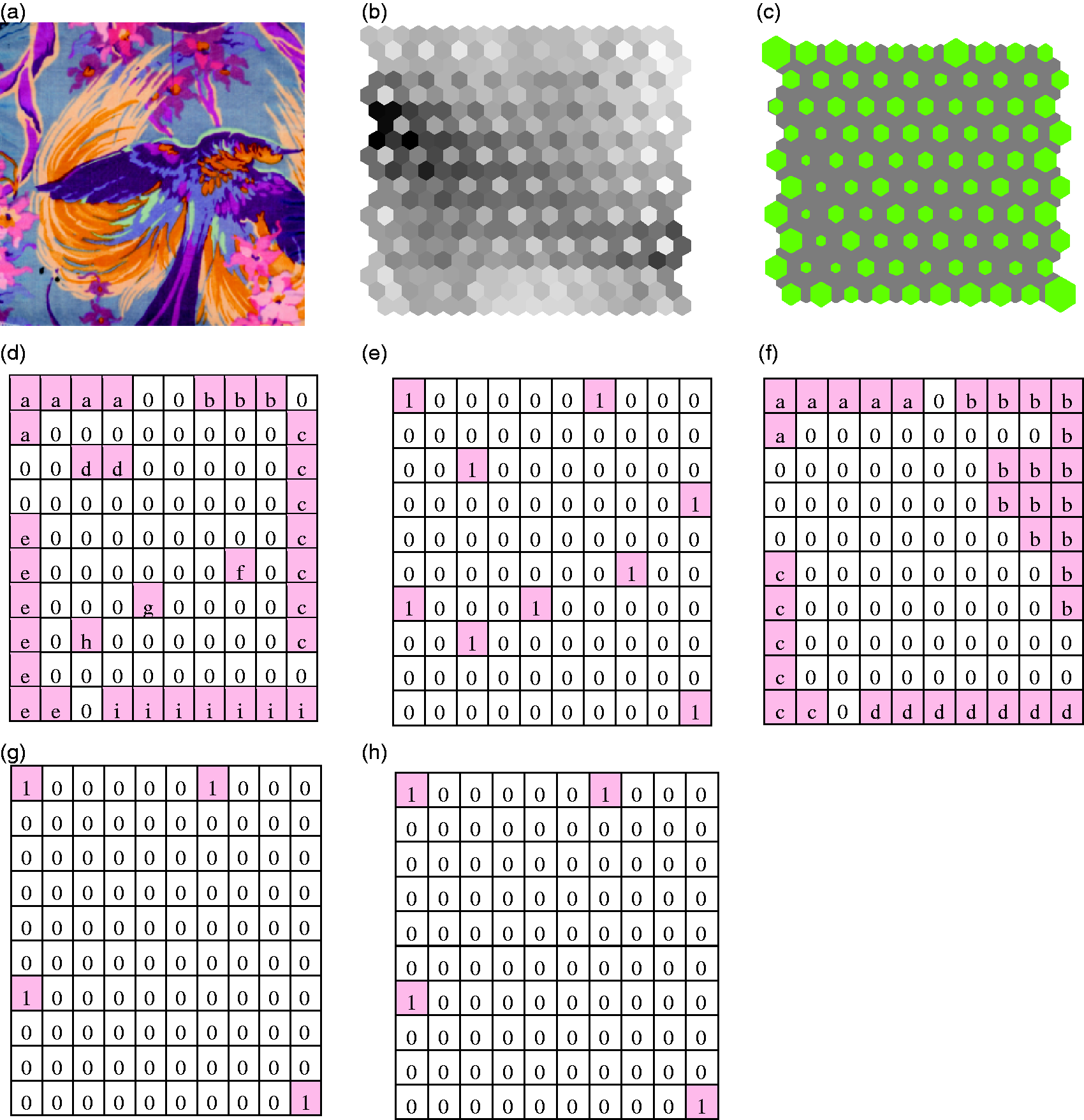

Cluster refinement

The coarse partition needs to be refined by segmenting the U-matrix with a more properly selected distance threshold than the average distance used in the coarse partition. The refinement can start with a large distance threshold, and repeat by decreasing the distance threshold until all the flagged neurons are assigned to different regions. In our application, the initial distance threshold, d, is set at 30 (or a larger number), which is far greater than the color difference that human eyes can easily perceive. As d decreases, the U-matrix will be segmented into more regions (clusters). When d reaches a value with which all the flagged neurons are used to label different clusters, the iterations stop. Let U1 be a matrix with the same size of the U-matrix, U, of a SOM. The cluster refinement can be executed in the following steps.

Step 1. Set initial distance d: d = 30.

Step 2. Partition U into different regions: merge the neighboring neurons into one cluster if the distance between them is less than threshold d.

Step 3. Assign a different number for each region.

Step 4. Create a new matrix, U1, by labeling each neuron with its region number.

Step 5. Decrease d: d = d − 1.

Step 6. Repeat steps 2–5 until all the flagged neurons have different labels.

Step 7. Take the current threshold d as the final threshold, β. The last U1 represents the refined cluster partition.

The above steps provide an automatic procedure to determine the distance threshold $(β)$ for the optimal cluster partition in a U-matrix. For image 1 in Figure 2, the calculated distance threshold, β, is 11, and the number of the partitioned clusters is 10, as exhibited in Figure 11. Figure 11 seems to over-segment image 1, which essentially has three major colors. In clusters 4 − 10, each contains a few pixels whose colors deviate from one of the three main colors, and should be merged into the cluster with the closest color or simply removed.

Figure 11.

Clusters in the refined partition of image 1: (a) cluster 1; (b) cluster 2; (c) cluster 3; (d) cluster 4; (e) cluster 5; (f) cluster 6; (g) cluster 7; (h) cluster 8; (i) cluster 9; (j) cluster 10.

Cluster merging

After the refined partition, the boundaries in the U-matrix are divided into smaller clusters with fewer hits. To avoid excessive segmentation, some of these clusters should be merged with their neighbors. For a pixel, q, in an image, it can have at most eight immediate neighbors. Let y denote the number of q’s neighbors that do not belong to the same cluster as q does, and z the ratio of y to the total number of q^’s neighbors. The dispersity of a cluster is measured by the average of all the z in the cluster. A cluster is regarded as ‘dispersed’ if its dispersity is larger than m₁. Figure 12 shows a cluster of four pixels (in triangles) surrounded by their neighbors (shown by crosses) that belong to other clusters. The dispersity of this isolated cluster is 0.625. This value, denoted as m₁, can be selected to threshold the dispersity. A cluster can be merged into its nearest neighboring cluster only when it is dispersed (dispersity > m₁) and the center-to-center distance to its nearest neighboring cluster is less than a preset threshold, m_2. m₂ is set at 30 in this application because it represents a highly noticeable color difference. The merging process is repeated until there is no longer any dispersed cluster in the U-matrix.

Figure 12.

A sample of a cluster whose dispersity is 0.625.

Figures 13–16 show the merging process of image 1. Figure 13(a) shows the refined partition of image 1, Figure 13(b) the distances between clusters and Figure 13(c) the dispersity of clusters. According to Figure 13(a), cluster 3 is surrounded by three neighbors (clusters 1, 4 and 7). Because the distance between cluster 3 and its nearest neighbor (cluster 4) is 8, which is less than m₂, they should be merged into one cluster. Then, recalculate the distances and the dispersity of clusters, and check the new cluster with clusters 7 and 1. When all the dispersed clusters are processed, a new partition result is attained, as shown Figure 14(a) (the clusters are renumbered). The final cluster distances between the three clusters are all above m₂, and the final dispersities are below m₁.

Figure 13.

Cluster dispersity: (a) the refined partition; (b) the cluster distances in the refined partition; (c) the cluster dispersity in the refined partition.

Figure 14.

(a) Merged clusters. (b) The final cluster distances. (c) The final cluster dispersity.

Figure 16.

The clusters and the reconstructed image of image 2: (a) cluster 1; (b) cluster 2; (c) cluster 3; (d) cluster 4; (e) cluster 5; (f) cluster 6; (g) reconstructed image.

Experimental results

The mean color value (center) of a cluster can be used to refill all pixels in the cluster. For image 1, the clusters segmented by the proposed SOM-based clustering algorithm and the FCM and the image reconstructed with these clusters are shown in Figures 15(a)–(d). Table 1 displays the mean color values in each cluster and their standard deviations (in parentheses). The three clusters segmented by the SOM and the FCM have almost identical shapes, although their color values differ slightly. There is no apparent difference between the two reconstructed images.

Figure 15.

The clusters and the reconstructed image of image 1. SOM: self-organizing map; FCM: fuzzy c-means.

Table 1.

The means and standard deviations of cluster colors of image 1

Cluster (colored region)	SOM			FCM
Cluster (colored region)	L	a	b	L	a	b
1	40 (18.23)	9 (7.85)	−10 (7.98)	35 (19.02)	8 (20.71)	−13 (8.46)
2	29 (6.63)	48 (7.60)	14 (6.42)	29 (16.89)	46 (4.70)	12 (6.03)
3	83 (6.62)	2 (2.37)	−1 (3.19)	65 (6.65)	6 (19.62)	−3 (13.37)

Note: the numbers in parentheses are the standard deviations.

SOM: self-organizing map; FCM: fuzzy c-means.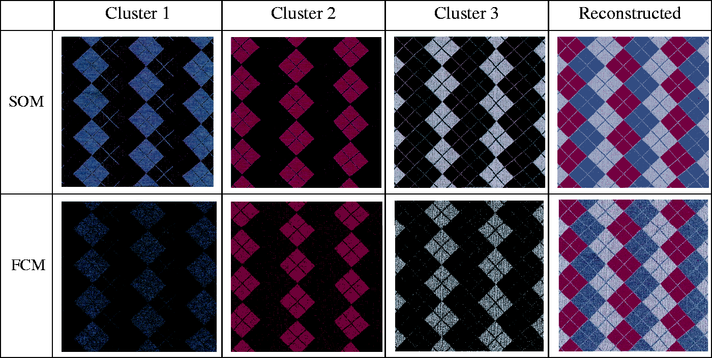

The color pattern of image 2 segmented by the SOM-based clustering algorithm comprises six colored regions (clusters), including four major colors (clusters 1, 2, 3 and 4) and two transitional colors (clusters 5 and 6). The clusters and the reconstructed image are shown in Figure 16. Table 2 shows the mean color value and standard deviations of each cluster, which can be used to evaluate color changes. Without the color segmentation, these discrete colored regions are nested, making an independent color evaluation impractical.

Table 2.

The means and standard deviations of cluster colors of image 2

Cluster (colored region)	L	a	b
1	20 (8.82)	34 (8.79)	−3 (9.49)
2	41 (13.20)	42 (10.25)	−17 (11.59)
3	61 (12.41)	41 (13.12)	16 (8.68)
4	62 (13.40)	31 (11.90)	65 (9.09)
5	78 (12.13)	11 (10.41)	22 (15.09)
6	50 (15.10)	5 (8.72)	−15 (9.35)

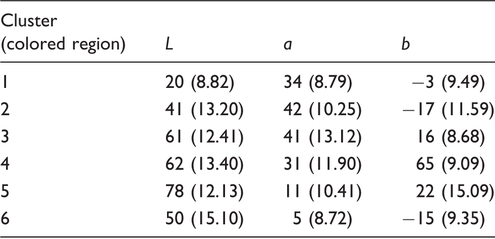
Note: the numbers in parentheses are the standard deviations.

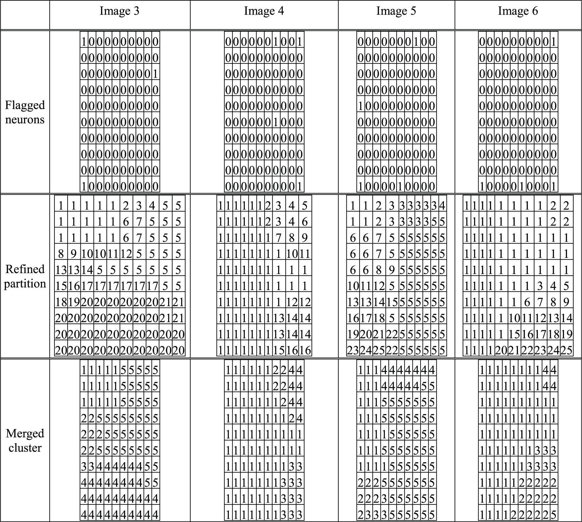
More sample fabric images were tested; their segmented color clusters are shown in Figure 17 and their Segmentation matrices in Table 3. Images 3 and 5 are printed multi-color fabrics, while images 4 and 6 are yarn-dyed fabrics. Except for image 4, color patterns in images 3, 5 and 6 have five main clusters. The mean cluster colors and their standard deviations are shown in Table 4.

Figure 17.

More sample fabric images and their segmented color clusters.

Table 3.

Color segmentations of images 3−6

Table 4.

The mean cluster colors of images 3–6 and their standard deviations

	Color space
	Image 3			Image 4			Image 5			Image 6
Cluster	L	a	b	L	a	b	L	a	b	L	a	b
1	56 (28.20)	−22 (9.08)	−18 (12.05)	61 (12.21)	5 (1.12)	13 (5.43)	36 (17.50)	60 (22.62)	−30 (12.19)	25 (18.69)	10 (11.94)	−22 (21.68)
2	83 (18.24)	−14 (12.79	−5 (16.73)	46 (9.43)	3 (1.29)	−2 (4.81)	88 (12.88)	−1 (26.94)	2 (8.25)	50 (16.51)	−7 (8.10)	−24 (16.54)
3	24 (15.29)	2 (5.69	−14 (12.66)	73 (9.21)	3 (1.46)	9 (7.77)	59 (15.00)	−20 (21.92)	−26 (11.87)	68 (13.88)	1 (9.19)	8 (14.92)
4	47 (26.17)	−8 (9.87	24 (10.54)	32 (9.37)	4 (1.32)	−9 (4.93)	27 (16.33)	34 (27.56)	−45 (11.13)	26 (17.31)	21 (8.39)	−4 (16.20)
5	63 (26.17)	−18 (9.74	37 (9.71)				36 (18.94)	2 (29.49)	−38 (13.44)	61 (16.55)	−10 (8.79)	48 (13.10)

Note: the numbers in parentheses are the standard deviations.

Summary

Color evaluation on a multi-color fabric requires the regions of different colors to be separated and measured individually. The SOM-based clustering algorithm presented in this paper can be used to automatically classify colors on multi-color fabrics and to accurately partition the regions of different colors. In the coarse partition, SOM neurons associated with the main colors are identified and flagged. In the partition refinement, the optimal distance threshold is selected when all the flagged neurons are assigned to different regions partitioned in the first step. In the cluster-merging stage, clusters with similar color characteristics are combined to avoid possible over-segmentation. This algorithm does not need to pre-define the number of clusters (e.g. main colors) and can automatically select a distance threshold to partition the U-matrix map that leads to precise segmentation of color patterns on a fabric.

In a future study, we will implement this SOM-based clustering algorithm for two applications: (1) printing quality assurance in which geometrical shapes and color values of individual colors are checked with the requirements; and (2) wash-fastness evaluation in which color changes of each color are examined after home laundering.

Footnotes

Declaration of conflicting interests

The authors declared no potential conflicts of interest with respect to the research, authorship and/or publication of this article.

Funding

The author(s) disclosed receipt of the following financial support for the research, authorship, and/or publication of this article: This work was supported by the China Scholarship Council (Grant Number: CZY12010).

References

AATCC Test Method 61-2013. Colorfastness to laundering: accelerated.

AATCC Test Method 8-2013. Colorfastness to crocking: crockmeter method.

Lin

. Automatic color identification in printed fabric images by a fuzzy-neural network. AATCC Rev 2002; 2: 42–45.

Macqueen J. Some methods for classification and analysis of multivariate observations. In: The 5th Berkeley symposium on mathematical statistics and probability, Vol. 1, Berkeley, 1967, pp.281–297.

Lim

Sang

. On the color image segmentation algorithm based on the thresholding and the fuzzy c-means techniques. Pattern Recognit 1990; 23: 935–952.

Gorji

Tehran

Rahmati

. New method for obtaining proper initial clusters to perform FCM algorithm for color image clustering. J Text Inst 2009; 100: 237–244.

. Feature encoding for unsupervised segmentation of color images. IEEE Trans Syst Man Cybern 2003; 33: 438–447.

Zheng

. A new method for automatic separation of fabric color. Text Res J 2015; 85: 1520–1538.

Luo

Shao

Shen

. An unsupervised method for dominant colour region segmentation in yarn-dyed fabrics. Color Technol 2013; 129: 389–397.

10.

Kohonen

. Self-organized formation of topologically correct feature maps. Biol Cybern 1982; 43: 59–69.

11.

Ultsch A. Self-organizing neural networks for visualization and classification. In: Conference on society for information and classification, Berlin, 1993, pp.301–306.

12.

Costa JAF and Netto MLA. Clustering of complex shaped data sets via Kohonen maps and mathematical morphology. In: SPIE conference on data mining and knowledge discovery: theory, tools, and technology III, Orlando, USA, 16 April 2001, pp.16–27.

13.

Patra JC, Abraham J, Meher PK, et al. An improved SOM-based visualization technique for DNA microarray data analysis. In: international joint conference on neural networks, Barcelona, Spain, 18–23 July 2010, pp.1–7.

14.

Costa JAF and Yin HJ. Gradient-based SOM clustering and visualisation methods. In: international joint conference on neural networks, Barcelona, Spain, 18–23 July 2010, pp.1–8.

15.

Sarlin P and Rennqvist S. Cluster coloring of the self-organizing map: an information visualization perspective. In: 17th international conference on information visualisation, London, UK, 16–18 July 2013, pp.532–538.

16.

Vesanto

Alhoniemi

. Clustering of the selforganizing map. IEEE Trans Neural Networks 2000; 11: 586–600.

17.

Zhang X and Li Y. Self-organizing map as a new method for clustering and data analysis. In: Internal joint conference on neural networks, Nagoya, Japan, 25–29 October 1993, pp.2448–2451.

18.

Ultsch A. U*-matrix: a tool to visualize clusters in high dimensional data. Technical Report No.36, University of Marburg, Germany, 2003.

19.

Kuo

Kao

Chiu

. Integrating a genetic algorithm and a self-organizing map network for an automatically separating color printed fabric system. Text Res J 2009; 79: 1235–1244.

20.

CIE. Colorimetry. 2nd ed. CIE Publication No. 15.2, 1986.

21.

Mathworks, MATLAB and the SOM toolbox. http://www.cis.hut.fi/projects/somtoolbox/ (accessed 23 November 2014).