Geography,policy or market? New evidence on the measurement and causes of sprawl (and infill) in US metropolitan regions

Abstract

This paper proposes four metrics to measure sprawl in metropolitan regions as marginal changes in land use over time. The metrics (change in urban housing unit density, marginal land consumption per new urban household, housing unit density in newly urbanized areas and percent of new housing units located in previously developed areas) are computed for all 329 metropolitan areas in the continental USA for 1980 and 2000. Regression analysis is used to explain variations in sprawl metrics across metropolitan areas, incorporating variables representing market, geographic and policy factors. Changes in development patterns reflect interactions of market and geographic structures. States with a substantial state role in planning accommodate a higher percentage of new housing units in previously developed areas and with lower marginal land consumption, suggesting that policy can mitigate sprawl development.

Keywords

growth management land use metropolitan sprawl urbanization

Introduction

Measuring and understanding the nature of urban spatial expansion is the subject of intense academic and popular interest. The literature on ‘sprawl’ has evolved to consider a wide range of measures, descriptions and causes and has utilized different data sources and methods, but has not achieved anything like scientific consensus (Cutsinger and Galster, 2006). While this paper does not provide definitive answers to this large and complex literature, it proposes a framework to think about measurement(s) of urban sprawl, offers multiple new data sources to implement these measures and presents multivariate estimates of the impact of different geographic, policy and market forces in explaining marginal changes in metropolitan land use patterns in the USA over 20 years.

Because sprawl is often conceptualised as a multidimensional phenomenon, measurement faces at least two inter-related challenges. First, to achieve analytical tractability, researchers either reduce the dimensionality of measurement through creation of indices, or focus on one dominant feature of land use patterns. The trade-off in empirical sprawl metrics is that multidimensional indices may conflate process, outcomes and causes, while single-dimension measurements may obscure these important inter-relationships. Trade-offs between conceptualisation and measurement may be driven by theory or by data availability. Reducing the dimensionality of a complex phenomenon does not have to be considered ‘reductionistic’ provided the research clearly describes these trade-offs and the measurements retain validity.

The second challenge, at least in the USA, has been the difficulty in obtaining temporally and spatially consistent land use data, able to be matched with socioeconomic, demographic and policy variables. If measures of sprawl reflect changes in land use patterns within an area, then empirical work requires data sources comparable across time and space and at the scale of the phenomenon being explained. This paper attempts to address these two challenges, both in the conceptual development of sprawl metrics and with the deployment of new data sources to measure and explain land use changes across US metropolitan areas.

This paper is organised as follows. First, the literature on urban sprawl measurement is outlined. This discussion argues for conceptual measurements of sprawl focused on relative and marginal changes in density, and four specific metrics of sprawl are proposed to reflect these concepts. The following section presents a discussion of the data sources and methods utilized to implement the metrics and the regression analysis of determinants of sprawl patterns. Then the results and discussions testing the impact of various geographic, policy and market forces in explaining differences in sprawl measures across US metropolitan regions are provided. Discussion and conclusions follow.

Concepts and measurement of ‘sprawl’

The word ‘sprawl’ – in its noun and verb forms – connotes a negative characterisation of spatial patterns of land development. However, as a scientific and policy concept it remains contested and poorly defined (Cutsinger et al., 2005; Ewing et al., 2002; Galster et al., 2001; Wolman et al., 2005). To review the voluminous sprawl literature is beyond the scope of this paper, but this review highlights five components of the measurement debate impacting the development of the proposed metrics. Questions of methodology include whether sprawl should be measured as a multidimensional phenomenon or whether it is valid to focus on one element. Second, can sprawl be measured in a cross-sectional framework as variation across places, or should it be measured in a time-series framework as changes within places? Third, is the appropriate measure of the concept of sprawl ‘average’ or ‘marginal’? Fourth, to what extent should measures of sprawl be integrated into stylised models of urban spatial structure? And, fifth, what spatial scale is appropriate for measurement?

Researchers presenting multidimensional indices of sprawl argue that sprawl is a complex phenomenon of both pattern and process such that understanding the interactions of pattern and process are necessary for policy relevance (Cutsinger and Galster, 2006; Cutsinger et al., 2005; Ewing et al., 2002; Galster et al., 2001). In the two extant research projects which advance multidimensional measures of sprawl (Cutsinger et al., 2005; Ewing et al., 2002) a large number of variables for each metropolitan area are collected and data reduction techniques are used to compute statistically valid indices for comparison across places. Ewing et al. (2002) combine multiple data sources for 83 metropolitan areas in 1990 and 2000. Using 22 variables from Census, employment, transportation and land use data bases, they use principal components analysis to identify four factors representing density, neighbourhood land use mix, activity centring and street-network accessibility. Each of these constructs is operationalised as that principal component that accounts for the maximum variance in the underlying variables. These four factors are scaled and combined into a ‘Sprawl Index’ to measure differences across metropolitan areas.

Cutsinger et al. (2005) and Wolman et al. (2005) update the data and methodology in Galster et al. (2001) and cover a sample of 50 metropolitan areas for 1990. Combining Census, transportation, employment and land cover data, they create 14 indices measuring sprawl along the dimensions of density, concentration, centrality, continuity, nuclearity (centres) and mix of uses. They then use principal components analysis to reduce these 14 indices to seven factors, which they label density/continuity, proximity, job distribution, mixed-use, housing centrality, nuclearity and housing concentration. The seven factors rank and compare metropolitan areas along each dimension of sprawl. The authors argue that different ordinal rankings across metropolitan areas confirm the multidimensional nature of sprawl that would be obscured in a single index.

In contrast, a large group of researchers have measured sprawl primarily in terms of density (Brueckner, 2001; Burchfield et al., 2006; Fulton et al., 2001; Glaeser and Kahn, 2004; Kahn, 2001; Lopez and Hynes, 2003; Malpezzi and Guo, 2001; Paulsen, 2012; Wassmer, 2006, 2008). Density can be population, housing-unit or employment density, and measurements include average densities, variations in densities or density gradients. Density measures focus on the dominant characteristic of sprawl and are more available in terms of data. Even within the literature measuring sprawl multidimensionally, variables representing density often play a strong role. In Ewing et al.’s (2002) index, the density factor accounts for two-thirds of the variance within the data set. Of the seven components identified by Cutsinger et al. (2005), the density/continuity factor accounts for the largest share of variance explained.

A second question of methodology concerns whether sprawl can be measured cross-sectionally or requires measurement over time. Even when theoretical understanding focuses on land use change, data availability has often forced cross-sectional measurements. Cross-sectional measures pose a challenge in interpretation because places have different histories and policy choices may be endogenous to observed land use differences. For example, density in New York is sometimes compared with Los Angeles, even though these two cities developed at different times in American industrial and settlement history. In Los Angeles, only 25% of the housing stock was built before 1950, compared with 50% in New York. If comparisons of land use patterns do not reflect historical differences, latter-developing cities by definition would be more ‘sprawled’ because they lack historically dense cores.

When sprawl is measured as a process in a time-series framework, metrics should characterise changes in land use patterns within a metropolitan area. Changes across places can still be compared, but only in relative terms. Consider again the New York/Los Angeles example. New York’s housing-unit density (per km² of urban land area, year 2000) is more than twice that of Los Angeles’ (1852 units/km² versus 897 units/km²). However, in the 20 years from 1980 to 2000, density in the Los Angeles area increased 48 dwelling units/km², while density in the New York metro declined 13 dwelling units/km². While New York is overall denser, new urban development in previously non-urbanized areas in the New York area occurs at lower densities than new urban development in Los Angeles.

Figure 1 illustrates this concept, showing a non-parametric regression of the natural log of population density on the distance to the metropolitan centre for urbanized block-groups in the New York and Los Angeles Primary Metropolitan Statistical Areas (PMSAs) in 2000. Regressing the log of population density on distance is a standard implementation of the ‘density gradient’ but non-parametric regression techniques do not impose any particular functional form on the output. New York fits the model of a traditional ‘centre-dominated’ city with a historically dense urban core and lower-density suburban areas. Los Angeles lacks a traditional ‘centre’ but is developed at more uniform and higher densities across the region. The suburban areas of Los Angeles beyond 13 miles (21 km) are developed at higher densities than similarly distant areas in New York.

Figure 1.

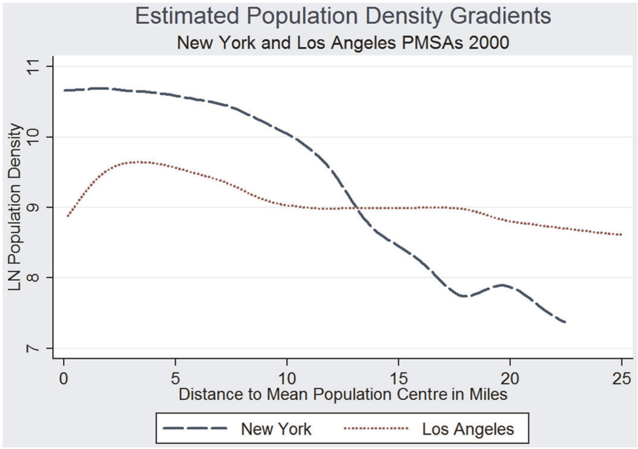
Population density gradients, New York and Los Angeles.

A third area of methodological concern is whether sprawl should be measured in average or marginal terms. In most discussions of sprawl, a common meaning is low-density development in suburbs or at the urban–rural interface. However, much research on sprawl measures the density across a metropolitan area (an average measurement), rather than the (marginal) density of newly developed land areas, or marginal land consumption per household. Marginal land consumption measures reflect a conceptualisation of sprawl as a process.

The fourth area of methodological difference is the extent to which researchers understand measurements to be rooted in models of urban spatial structure. Consider the standard model of spatial structure in urban economics, the monocentric or Alonso-Mills-Muth (AMM) model. Development densities within a region reflect land prices, as different uses compete for accessibility to the central business district. The emergent pattern of land use is the envelope of each use’s bid-rent curve. Land values, and hence development densities, decline with distance to the centre. The spatial extent of urban development is increasing in population and income, and decreasing in agricultural land prices and transportation costs (Brueckner and Fansler, 1983; McGrath, 2005; Paulsen, 2012; Spivey, 2008; Wheaton, 1974).

Despite its overly simplified model structure, the monocentric city model continues to explain a large percentage of variation in development patterns across US areas (Malpezzi and Guo, 2001; Paulsen, 2012; Spivey, 2008; Wassmer, 2006). In the context of this stylised model, increases in population and income are expected to lead to outward urban expansion. Should we therefore understand all spatial expansion of the development area of a city as ‘sprawl’? Urban economist Jan Brueckner argues from this model that we should only label ‘excessive’ spatial expansion of urbanized areas as ‘sprawl’ (Brueckner, 2001). Urban spatial expansion is ‘excessive’ when one or more policy or market failures extends land development further out than would otherwise be socially optimal. There is yet no agreement how to measure the welfare losses of habitat loss, traffic congestion or other impacts of sprawl, so there is no agreed-upon method to identify the ‘optimal’ size of urbanized areas (Cheshire and Sheppard, 2004). But the intuition behind this argument is that not all expansions of urban areas constitute ‘sprawl’. When sprawl is measured as marginal changes in land patterns and densities across places, comparisons could show that one place is more ‘sprawling’ than another, while not directly testing or measuring whether such spatial expansion is ‘excessive’.

The fifth concern of methodology considers the spatial scale at which sprawl is measured. Most of the research cited above uses metropolitan statistical areas. Even when land use data is derived from non-Census sources, the metropolitan area is used to represent the economic integration of rural areas with one or more central (principal) cities. Metropolitan areas are based on county boundaries, so a county with some economic integration (commuting) with the central city would be included even if it contains significant amounts of rural and/or undeveloped land. Metropolitan area boundaries are often used because of the wider range of data available and because these boundaries include ‘rural’ or ‘exurban’ sprawl: (very) low-density development at the fringe without urban-type services (water and sewer connections).

Alternatively, a number of researchers within the urban economics tradition use the ‘urbanized area’ boundaries of the Census (Spivey, 2008; Wassmer, 2006, 2008). Their measures focus on sprawl as ‘urban decentralization’ (Wassmer, 2008: 537) but exclude (very) low-density development outside of ‘urban areas’ by definition. Wolman et al. (2005) and Cutsinger et al. (2005) argue that metropolitan area definitions ‘overbound’ sprawl because including rural areas upwardly biases sprawl indicators. Likewise, they argue that urbanized area boundaries ‘underbound’ sprawl because some amount of rural or fringe development is not included. Instead, they propose a measurement called the ‘extended urban area’ (EUA) as the Census-defined ‘urbanized area’ plus ‘each additional outlying square-mile cell … [within the] metropolitan statistical area that has 60 or more dwelling units and from which at least 30% of its workers commute to the urbanized area’ (Cutsinger et al., 2005: 237).

The research presented here focuses on measuring ‘urban’ sprawl (as incremental urban expansion) and would therefore necessarily exclude or ‘underbound’ what some would call ‘rural sprawl’. The results of this research should therefore be understood in this context and not as a complete measure of all land use change and development. There is a large and growing literature on measuring and defining rural sprawl, which argues that rural housing development is driven by amenities more than proximity to employment (Deller et al., 2001; Esparza and Carruthers, 2000; Radeloff et al., 2005). ‘Urban’ sprawl therefore has different drivers and policy responses than ‘rural’ sprawl. The purpose of this paper is not to diminish or ignore concerns about rural sprawl, but rather to develop conceptually robust and empirically implementable measures of urban sprawl.

As noted by Wassmer (2008), most of the independent variables needed for explanatory models are not available or measureable at the ‘EUA’ level. The approach used in this paper is therefore to present measurement of sprawl as changes in ‘urban’ areas within the spatial extent of each metropolitan statistical area. While based on the Census approach to ‘urban area’ classification, the approach here (described in detail in the section ‘Data and methods’) does not impose the minimum population size of 50,000 for an area to be considered urban, thus mitigating some (but not all) of the concern of spatial boundaries.

This paper operationalises four metrics of sprawl to measure relative (not absolute), marginal (not average) changes in density over time (not cross-sectional) in metropolitan areas, embedded within a framework derived from the monocentric model. Because of the need for analytical tractability metrics are computed in terms of housing-unit density.

Theoretical development of the sprawl metrics in this paper requires more detailed consideration of the implications of the monocentric city model, illustrated in Figure 2 with actual data from the 100 largest metropolitan areas for 1980 and 2000. Like Figure 1 above, shown is a non-parametric regression of the natural log of population density on the distance from the centre of each metropolitan area. This analysis combines hundreds of thousands of census block-groups to illustrate a ‘standardized’ or ‘equilibrium’ pattern of urban form across US metro areas. The shape of the density gradient is stable over the 20 years of this study. Consistent with theory (increasing population and increasing real income), the density gradient shifted upward and outward from 1980 to 2000. New land on the urban fringe was converted to urban development (outward shift), and additional development density was added to lands already considered urbanized in 1980 (upward shift).

Figure 2.

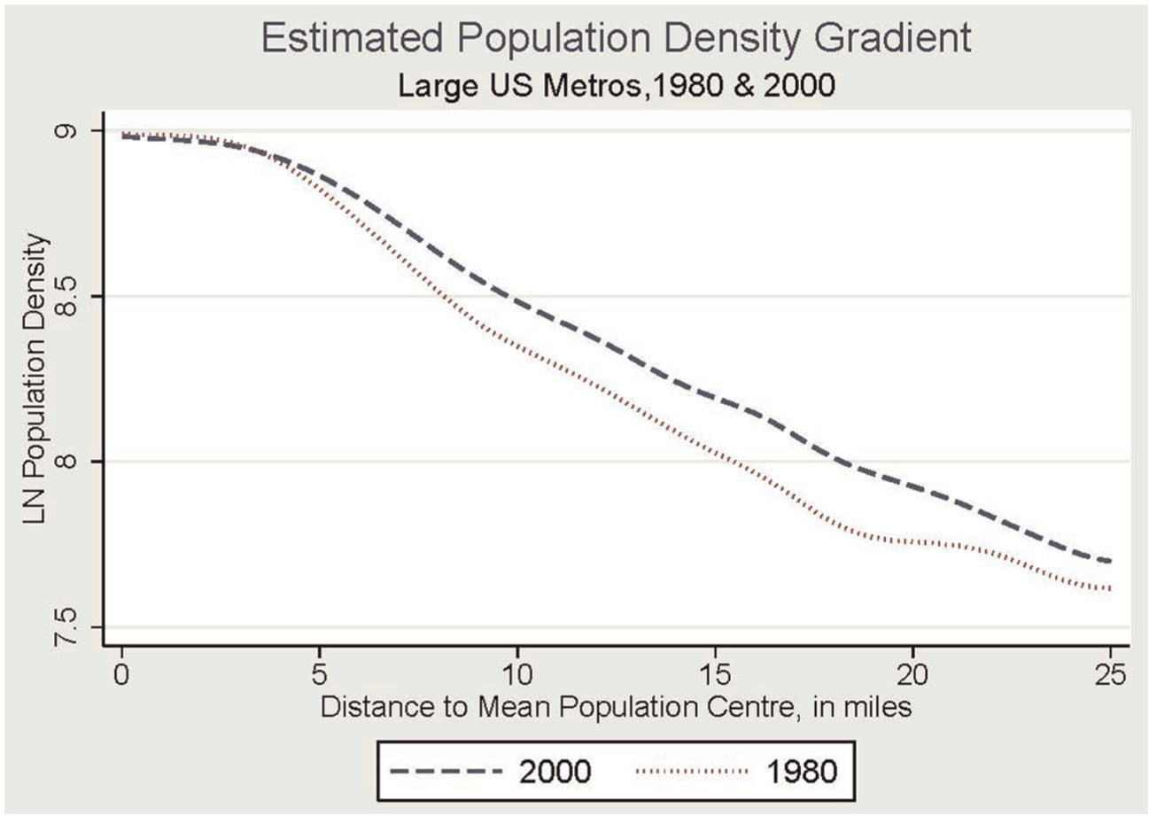
Population density gradients, US large metropolitan areas.

Consider Figure 3 which is a stylised representation of the model, showing the spatial extent of urban development shifting from X ₁ to X ₂ (X ₁ > X ₂). The right panel of Figure 3 shows that, from a ‘bird’s-eye view’, the spatial extent of urban development appears as a circle of radius X ₁ and, later, X ₂. 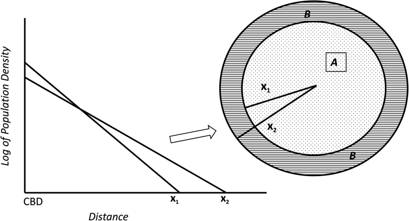In the first time period, the area of urban development, labelled as the dotted area A, is given by: $A = π X_{1}^{2}$ . The area newly converted to urban development from time 1 to 2 on the urban fringe is labelled as the lined-area B. The new area of the city, A+ B, is now A+B = $π X_{2}^{2}$ .

Figure 3.

Illustration of urban spatial expansion.

To implement metrics of sprawl reflecting marginal land consumption and changes in land use patterns, the metrics presented here capture changes in density gradients, the change in urban area extent from X ₁ to X ₂, and the density of development in areas labelled B in Figure 3.

(1) Change in housing-unit density. Housing-unit density in the first period (1980) is computed as H ₁/A; housing units divided by urbanized area. Housing-unit density in the second period (2000) is given by H ₂/(A+B). The change in housing-unit density, representing the change in the slope of the density gradient, is therefore given by [H ₂/(A+B)] − [H ₁/A].

(2) Marginal land consumed per net new urban housing unit is given by (H ₂− H ₁)/B. This measures the efficiency with which a metropolitan area accommodates new households. If new housing units are built in areas already considered urban (area A in Figure 3), the marginal (urban) land consumption for that housing unit is 0. For new housing units constructed in newly urbanized areas (area B in Figure 3), marginal land consumption is measured as the area of B divided by the number of housing units in B. As a metric calculated over the entire metropolitan area, this measurement combines the percentage of new housing units added to previously urbanized areas and the density of lands newly urbanized.

(3) Housing-unit density in newly urbanized areas. This metric directly measures marginal changes in land use. Referencing Figure 3, this metric is the density of housing units in newly urbanized areas, area B. One advantage of the data set used in this paper is that the data are at the block-group level, permitting direct measurement of the actual number of housing units in newly developed areas. Such measures were not previously possible with remote-sensed sources.

(4) Percent of net new urban housing units in previously urbanized areas. This measure proxies ‘infill’ (or the inverse of sprawl): areas with higher percentages of new urban housing units accommodated in previously urbanized areas are less sprawling. Because, as above, the data used to develop measures are built-up from block groups, the net increase in housing units in areas previously classified as urbanized in the first time period (1980) can be measured. A block-group might reach the population density threshold to be considered urban in 1980, while still having vacant or undeveloped land on which new housing could be built. This measure captures both what planners traditionally would call ‘infill’ (development or redevelopment on previously developed lands) and what can be called ‘near-fill’ (urban development directly adjacent to or within the same census block-group as already developed land).

Data and methods

Previous research has been limited by nationally available data measuring both land use change and population variables in temporally and spatially consistent units. Even when sprawl has been conceptualised in dynamic and marginal terms, data limitations have required empirical implementation with static or average metrics.

For measures of land use patterns (as the denominator in density calculations), researchers have relied either on Census data or on measures of developed land area from remote-sensing or surveys. While increased sophistication of remote-sensing and image processing opens the possibility of more refined measures of land use patterns in the future, the only consistently interpreted satellite-derived measurement of urbanized land area extent is the National Land Cover Database (NLCD) Change Retrofit project, covering 1992 and 2001 (Fry et al., 2009). USDA’s National Resources Inventory (NRI) is sample-point data on land uses in 5-year intervals from 1982 to 2007. NRI data are no longer available publicly while the methodology is revised and updated. Because NRI data are derived from samples, confidence intervals on small-area measurements are often quite large and statistically problematic. NRI and NLCD data, while useful in describing changes in land use patterns, are also not easily able to be matched to Census geographies where employment, transportation, household or population data are available.

The alternative approach to measuring land use patterns involves Census data itself. Implementing change analysis has been problematic because Census geographies and definitions change with each decennial census. Matching Census geographies across time and space is necessary to ensure that measures reflect real changes and not changes in areal units. The Census construct most closely representing the spatial extent of urban development (or ‘urban footprint’) is delineation of areas as ‘urban’ (‘urbanized areas’ and ‘urbanized clusters’). The Census classifies areas as ‘urban’ based on population density thresholds and proximity to other densely developed areas. The difficulty for sprawl metrics is that the definition and classification method for ‘urban’ has changed every decade and is scheduled to change again in the 2010 release.

The research presented in this paper overcomes these challenges by utilizing a newly published data set on US urbanized land area (Paulsen, 2012) using historically consistent census block-group boundaries and applying the Census 2000 urban area determination algorithm (described below) retroactively and consistently to 1990 and 1980 data. Each census block-group within a metropolitan area (using data in consistent year-2000 boundaries) is classified as whether or not it is ‘urban’ in 1980, 1990 and 2000. In terms of the discussion in Figure 3, these data permit measurement of the exact size of areas A and B for all 329 metropolitan statistical areas (MSAs and PMSAs) in the continental USA for 1980 and 2000, as well as the ability to count the number of housing units in each area for each time period. This 20-year time period is used to measure marginal changes in urban form.

The methodology and algorithm to develop urban-extent measures is described in detail in Paulsen (2012). All block-groups with a population density of 1000 persons/mile² (386 persons/km²) are identified as constituting an urban core. Then, adjacent block groups (allowing for up to half-mile ‘jumps’ as per the Census) with a population density of 500 persons/mile² (193 persons/km²) are additionally classified as urban. This algorithm repeats in half-mile buffers until no adjacent block-groups meet the density threshold of 500 persons/mile². There is no minimum total population requirement to classify an area as urban. This method is repeated for each time period and the resulting product is a measure of the total area considered ‘urbanized’ within each metropolitan area. Within each urbanized area, detailed calculations of changes in housing units and population can be made over time. Metropolitan areas may have more than one urbanized area.

The minimum population density to be considered ‘urbanized’ is therefore 500 persons/mile². Even assuming a smaller-than-average household size of two persons per housing unit, and expressed in terms of land consumption per housing unit (the inverse of density : land area divided by housing-units) this measure would capture housing units developed at 2.56 acres/house (1.04 ha/house). This measure thus partially addresses the ‘underbounding’ issue in capturing very low-density suburban development.

Sprawl metrics presented in this paper measure housing-unit density in these classified ‘urbanized’ areas, summarised over each metropolitan area. Housing-unit (rather than population) density is utilized as a durable and tractable measure of urban spatial form. Each of the four sprawl metrics described in the section ‘Concepts and measurement of “sprawl”’ (change in housing-unit density, marginal land consumption per net new housing unit, density of housing units in newly urbanized areas, and percent net new housing units in previously urbanized areas) are calculated for each of the 329 metropolitan areas used in this analysis. Because of space constraints, rankings of metropolitan areas on these four metrics are not presented, but are available upon request.

Ordinal rankings of metropolitan areas vary significantly across metrics, indicating that combining variables into a singular sprawl metric could obscure significant variation. Although ordinal rankings vary, there is some degree of correlation across the metrics, as expected. The highest correlation (Pearson r = −0.84; Spearman’s rho = −0.76) is between the marginal land consumption metric and the percent of units in previously urbanized areas. This is inherent to how these metrics are computed. Marginal land consumption per household is a direct function of two other metrics (percent in previously urbanized areas and density in newly urbanized areas). There is still value in using each metric separately in the regression analysis because of different significant independent variables. However, interpretation should proceed with understanding that these metrics are not completely independent of each other.

As a test of the informational added-value of the marginal metrics (2, 3 and 4) relative to the average metric (1−change in average density), correlation tests were performed. The most significant correlation with the first metric was with metric 3, density of development in newly urbanized areas (Pearson r = 0.44; Spearman’s rho = 0.30). These correlations do show the durability of metropolitan-specific density paths, but also demonstrate that marginal metrics add additional information to characterise changes in metropolitan spatial patterns.

Multivariate analysis consists of regressions where the four metrics of sprawl are dependent variables. The purpose of the regressions is to explain variation in sprawl across areas, utilizing as controls a number of independent variables which theory and previous literature have shown to significantly affect land development patterns. For purposes of presentation, these independent variables can be categorised as ‘market’, ‘geographic’ and ‘policy’ factors, even though variables could be considered in more than one category.

To the extent that land development reflects market forces, explanation of changes across places includes variables reflecting prices, income and demographic demand factors. Median household income in 1980 (in 1999 US$) is included. Land price data is represented by the average value of agricultural land in each metropolitan area, based on Census of Agriculture county-level data. The value of agricultural land in each metro is a weighted average (by county size) of county-year observations of price data on each side of the decennial census population observation. For example, 1977 and 1982 agricultural values are interpolated and weighted by county-size to reflect average metropolitan land values for 1980. Land data are inflation-adjusted to 1999 dollars. Variables representing demographic demand characteristics include percentages of housing units owner-occupied and the percentage of residents over the age of 65. Also included is a measure of the share of the metropolitan population of racial or ethnic minorities. This variable is calculated as 1 minus the share of non-Hispanic whites in 1980. Although there is a literature on the effects of sprawl on racial segregation (see Galster and Cutsinger, 2007; Rothwell and Massey, 2009) this variable is more of an indirect test of the effects of racialised land use decision making. Do jurisdictions in areas with higher minority populations adopt land use regulations to lower densities in order to exclude minorities (Pendall, 1999, 2000)?

In terms of geographic variables, two variables reflect the historical evolution of metropolitan structure: housing-unit density for 1980 and the percentage of housing units built before 1950. Controls for metropolitan land area test whether growth patterns differ by city size. Also included is a measure of land availability for development, the percent of the metropolitan area considered ‘undevelopable’. Although some measures of topographic constraints or coastal proximity have been utilized in previous sprawl research, the particular combination here (including ‘protected lands’) has not. The measure of undevelopable land area consists of three separate layers. First, NLCD 2001 national data is used to identify lands classified as water or wetlands. Second, using the EDNA (Elevation Dataset for National Applications) product, areas with greater than 15% slope are identified. Both NLCD and EDNA products are 30-m resolution and cover the entire USA. Third, the Protected Areas Database of the US (PAD-US) is utilized. The USGS GAP analysis program supervises and verifies this data, and federal, state, local and non-profit lands with GAP codes of 1, 2 or 3 (indicating permanent protection from land cover conversion) are coded as ‘protected’ and therefore unavailable for development. Using geospatial overlay analysis to prevent double counting, these three land features (water/wetlands, steep slopes and permanent protection) are added together to measure the percent of land in each metropolitan area undevelopable. Because this measure includes federal lands and not just topographic constraints, it identifies important forces shaping metropolitan growth patterns. Recent work by Saiz (2010), for example, measures geographic constraints on housing supply with topographic features (slopes and water area) but not protected land areas. In the data set presented here, the metropolitan area with the largest percentage of land undevelopable is Las Vegas, driven by federal land holdings.

In terms of policy variables, two concepts frequently included in the literature are fragmentation and growth management. Local government fragmentation is frequently linked to sprawl outcomes (Carruthers and Ulfarsson, 2002; Mills, 2006). The general hypothesis in the literature is that greater levels of fragmentation are associated with increased sprawl. Following the literature, fragmentation is measured here as the number of general-purpose local governments per 1000 population (year 2000 population).

Three variables measure regional or state planning for growth management to reduce sprawl. First, data on urban containment as collected by Nelson and also utilized by Wassmer (Nelson et al., 2007; Wassmer, 2006) measure whether a metropolitan area had a regional ‘urban containment’ policy in place during the time from 1980 to 2000. Although this variable has shown mixed results in empirical work (Paulsen, 2013), it is one of the most widely available and widely used metrics of regional growth management. This variable is available for all 329 metropolitan areas and is implemented as a dummy variable equalling 1 for regions with urban containment. Alternative specifications measuring the number of years such containment was in place did not alter results and are not reported.

An alternative measure of growth management planning which has been utilized is to measure the strength of each state’s planning system in supervising and regulating local land use planning. This data was developed by the American Planning Association and the Institute for Business and Home Safety based on analysis of state planning enabling laws and frameworks. Each state’s role in managing local planning is classified as ‘weak’, ‘significant’ or ‘substantial’. A dummy variable for those states with a ‘substantial’ state role (California, Florida, Maryland, New Jersey, Oregon, Rhode Island and Washington) is used to test whether stronger state planning frameworks alter land development patterns.¹ Because a strong state planning role and regional containment policies may complement each other, they both enter into the regression analysis as policy variables.

Alternatively, the Wharton Restrictions Index (WRI) is a measure of the overall restrictiveness of residential land development within a region, but is only available for the largest 94 metropolitan regions (Gyourko et al., 2008; Saiz, 2010). The version of the index reported in Saiz (2010) is used here, and is constructed to represent multiple dimensions of land use restrictions in a consistent scale, higher numbers indicating a more restrictive development environment. In the regression results reported below, separate regressions utilizing the WRI are estimated because the urban containment and state planning roles are included in the WRI index. For each dependent variable, therefore, two models are estimated: one with the containment/state policy variables and a separate one (for only 94 metros) for the WRI.

The regression results for the eight models are reported in Table 1. The format of each of the regressions is the same: the measure of sprawl or land use change from 1980 to 2000 is regressed on independent variables measured at the beginning of the time period (1980). Diagnostic tests indicate mutlicollinearity is not a problem (highest VIF is below 3). Diagnostic tests indicate the presence of heteroskedasticity, so each regression is estimated with robust standard errors. R ² measures of fit perform better in the sample restricted to the 94 largest regions with WRI data, suggesting the possibility that metrics developed from stylised urban models are more reflective of larger cities.

Table 1.

Regression results.

	Change in urban housing unit density		Marginal land consumed per net new urban household		Density of housing units in newly urbanized areas		Percent of net new urban housing units in previously urbanized areas
Median household income (1980, in thousand 1999 US$)	−1.4544000	0.2506957	−0.0000207	−0.0000195	6.1206523	9.3741620	0.0061077	0.0081683
	[0.379]	[0.914]	[0.121]	[0.180]	[0.188]	[0.147]	[0.037]**	[0.002]***
Average metropolitan agricultural land value (1980)	0.0058258	−0.0086585	0.0000000	0.0000000	−0.0005509	−0.0116406	0.0000044	−0.0000052
	[0.022]**	[0.199]	[0.652]	[0.138]	[0.959]	[0.419]	[0.353]	[0.356]
Percent of land undevelopable	80.0953000	101.7160000	−0.0001322	−0.0001878	−125.1751934	−190.4081668	0.1424560	0.1925464
	[0.014]**	[0.078]*	[0.609]	[0.547]	[0.042]**	[0.146]	[0.016]**	[0.009]***
Metropolitan land area	0.0038030	0.0016593	0.0000000	0.0000000	0.0221794	0.0275823	−0.0000034	−0.0000078
	[0.308]	[0.733]	[0.311]	[0.717]	[0.016]**	[0.020]**	[0.070]*	[0.000]***
Urban housing unit density (1980)	0.0164579	0.0426112	−0.0000001	0.0000000	0.2568839	0.1125679	−0.0000253	−0.0000179
	[0.611]	[0.150]	[0.374]	[0.946]	[0.022]**	[0.223]	[0.292]	[0.491]
Metropolitan percent minority (1980)	−45.8604000	−105.6270000	0.0003225	0.0003414	−227.3869667	−19.8022727	0.0228686	0.0435352
	[0.471]	[0.339]	[0.464]	[0.541]	[0.064]*	[0.923]	[0.820]	[0.724]
Percent residents over 65 (1980)	40.9785000	353.3060000	−0.0012707	−0.0040125	649.3222460	1834.2702916	−0.1956965	0.4953948
	[0.889]	[0.517]	[0.410]	[0.040]**	[0.232]	[0.044]**	[0.610]	[0.231]
Percent housing units owner-occupied (1980)	−168.5700000	−548.1040000	0.0034560	0.0062900	−278.2677693	−1139.0300000	−0.8275556	−1.0842388
	[0.238]	[0.018]**	[0.001]***	[0.001]***	[0.332]	[0.089]*	[0.001]***	[0.008]***
Percent of housing units built before 1950	−237.3470000	−243.7070000	0.0006284	0.0015014	−1375.0700000	−1424.0500000	0.4191724	0.2744544
	[0.002]***	[0.136]	[0.282]	[0.040]**	[0.000]***	[0.000]***	[0.003]***	[0.079]*
General purpose governments per 1000 population	1.2865500	−2.0674800	−0.0000109	−0.0000035	0.8164979	5.8806456	0.0023499	−0.0022705
	[0.035]**	[0.450]	[0.006]***	[0.817]	[0.443]	[0.215]	[0.036]**	[0.484]
Substantial state planning role (dummy)	25.1778000		−0.0002696		77.5932591		0.0464184
	[0.256]		[0.042]**		[0.191]		[0.099]*
Urban containment (dummy)	−10.0744000		0.0000112		−59.5524861		−0.0037233
	[0.619]		[0.924]		[0.201]		[0.873]
Wharton Restrictions Index (WRI)		11.0653000		−0.0002317		49.6729743		0.0296547
		[0.549]		[0.019]**		[0.128]		[0.202]
Constant	151.8960000	366.1930000	−0.0000099	−0.0021962	364.6731142	804.8864853	0.8603074	0.9636018
	[0.087]*	[0.061]*	[0.989]	[0.132]	[0.081]*	[0.087]*	[0.000]***	[0.001]***
Observations	329	94	317	94	300	93	317	94
R ²	0.169	0.371	0.121	0.401	0.408	0.602	0.181	0.47

Robust p values in parentheses.

Significant at 10%; **significant at 5%; ***significant at 1%.

The first two columns report change in housing-unit density as the dependent variable. Positive (negative) numbers indicate that average housing-unit density within the metropolitan area increased (decreased) over the time period. In the full sample, positive coefficients on agricultural land prices are in keeping with expected land market effects: areas with higher valued land increased density over the 20-year time period, all else being equal. Metropolitan areas with a greater percentage of their land base undevelopable also saw housing-unit density increases. Consistent with Figure 2, older centre-dominated regions (greater percentage of housing before 1950) saw density gradients flatten (reduced average density.) Metropolitan spatial patterns clearly respond to land market signals expressed in prices and supply constraints.

The second set of regressions (columns 3 and 4) involve marginal land consumed per net new urban household. Recall that this measure incorporates both the density of housing units in newly developed areas and the percent of housing units as ‘infill’, and therefore measures the overall land efficiency of a region in accommodating new housing units. Consistent with Fischel’s (2001, 2004) ‘homevoter hypothesis’ (areas with a higher percentage of housing units owner-occupied are more likely to zone to protect property values by restricting density of new development), regions with a higher percentage of units owner-occupied consumed more land per net new housing unit.

In terms of policy variables, both the dummy variable for a substantial state planning role and the WRI are significant and negative, indicating that each net new housing unit consumes less land than housing units in weaker planning states or lightly regulated regions. For advocates of a stronger state or regional role in managing local planning and growth, these results are consistent with the idea that stronger planning institutions can potentially reduce sprawl or promote more efficient land development patterns (Paulsen, 2013). As seen when comparing across the next regressions, a stronger state role in managing growth reduces marginal land consumption per household not by affecting the density of new housing development but in (re)directing growth to already urbanized areas.

In terms of the density of housing in newly urbanized lands (columns 5 and 6), a number of variables reflecting market conditions and patterns of urban growth are significant. Larger metropolitan regions and regions with higher initial densities saw denser development in newly urbanized areas. Conversely, older regions (greater percentage of housing built before 1950) and more supply-constrained lands (percent undevelopable) saw lower-density development. The negative coefficient on percent undevelopable is perhaps surprising. Comparing across to other metrics, areas with a greater percentage of land unavailable for development see overall densities increase because a greater proportion of new development occurs in already urbanized areas. In one sense, then, land supply restrictions function as a ‘natural’ urban containment or growth management strategy (Nelson et al., 2007). However, land supply constraints result in lower-density development in newly urbanized areas. These results are somewhat consistent with Saiz (2010) who finds that regions with more land supply constraints are more likely to adopt more restrictive development policies.

The variable measuring the percent of minority residents shows a negative relationship with marginal densities in newly urbanized areas. Interpretation of this coefficient requires some caution because its significance level is higher than 0.05. This negative coefficient would indicate that, all else being equal, housing development in newly urbanized areas is lower in regions with a larger minority population. The most likely explanation and mechanism for this result is that communities at the edge of urban development (suburbs) zone at lower densities to reduce the potential that minority households might move into their communities. This evidence would be consistent with the long-standing concern that lower-density zoning may have racially exclusionary intentions or effects (Galster and Cutsinger, 2007; Pendall, 2000; Rothwell and Massey, 2009).

The final two columns explain variations in metropolitan ‘infill’ patterns, the percent of new housing units in previously urbanized areas. Higher income areas show higher demand for infill, while a higher percentage of homevoters (owner-occupied units) is negatively related to infill. As expected, a higher percentage of the land base undevelopable (supply limitations) is associated with a higher degree of infill. Although this result is consistent with previous results indicating that physical constraints to development can act as either complements or substitutes for ‘growth management’ (Nelson et al., 2007; Saiz, 2010), expansion of this measure to include protected areas could also suggest that policies promoting land preservation and conservation can lead to more compact urban development (Daniels and Lapping, 2005). The positive coefficient on a substantial state planning role indicates that states with greater supervision and regulation of local planning and development accommodate a greater percentage of new urban housing units in already urbanized areas.

Discussion and conclusions

Changes in spatial development patterns over time reflect the interaction of land markets and geographic structures, spatial patterns and each region’s historical evolution. Worldwide, many cities appear to reflect the forces of dispersion and decentralization (Anas et al., 1998) particularly as transportation costs decline and the necessity of concentrating employment in urban centres is eroded (Glaeser and Kohlhase, 2004). Certainly that has been true in the USA, as shown in Figure 2. Cities in the USA expanded in land area during the years studied, 1980–2000. For these 329 metropolitan areas, nearly 51,000 km² of land was converted to urban development and 18.5 million net new urban housing units were constructed. Over 12.1 million of these new urban housing units (65%) were accommodated in areas already classified as urban in 1980. The four metrics proposed here try to capture these land use changes as relative, marginal and dynamic phenomena and reveal important structural relationships in metropolitan development across the USA, including policy initiatives to manage or reduce sprawl. Before ‘sprawl’ can be remediated or constrained, there needs to be conceptual clarity on how to measure sprawl and its relationship to metropolitan structure. The metrics proposed in this paper are one way to conceptualise sprawl, but certainly not the only way.

Policies to constrain sprawl have generally been labeled ‘Smart Growth’ or ‘growth management’ or ‘urban containment’, and this research offers some insight concerning these policy instruments. First, the statistical insignificance of the variable measuring urban containment should not be taken to mean that urban containment policies do not affect spatial patterns of land development. Rather, it is possible that this widely used measurement, implemented as a dichotomous dummy variable, does not reflect important variations within containment regimes. Some regions coded as having containment, such as Portland, have strict urban growth boundaries. Others use a more growth-accommodating urban service area approach. The institutional complexity across containment regimes cannot probably be captured by existing measures (Paulsen, 2013).

Second, the significance of the variable ‘substantial state planning role’ is consistent with the idea that when local governments are required to prepare comprehensive plans and/or prepare growth management plans consistent with state policy objectives, urban development can be accommodated in a more compact manner. The results suggest that greater land use efficiency in states with stronger planning is due to more development being directed to already developed areas, rather than more dense development in fringe areas. Likewise, areas which have more restrictive land development regulations (WRI) accommodate new housing units with greater land efficiency. Areas where a greater percentage of the land area is unavailable for development show increases in density and accommodate more of new development in previously urbanized areas.

These three policy measures – strength of state planning role, WRI and percent of land available for development – all are suggestive of the potential that increased regional or state planning and regulation can reduce, at least in part, some of the land consumptive impacts of urban development. If sprawl is conceptualised as marginal changes in density over time within a metropolitan area, the evidence here is consistent with the idea that some policy interventions can reduce the marginal land consumption associated with additional urban households. The metrics and analysis presented here, however, cannot measure the welfare effects or costs of regional growth management policies, something on which research has yet to achieve any consensus (Anas et al., 1998; Cheshire and Sheppard, 2004; Downs, 2004).

Footnotes

Acknowledgements

I thank the anonymous reviewers for many helpful comments which clarified my thinking. I want to thank colleagues Jack Huddleston, Steve Malpezzi and Annemarie Schneider for helpful conversations. I thank Sandra Poppenga of the Topographic Science unit in the Earth Resource Observation and Science (EROS) Center of the US Geological Survey for providing the EDNA data. Andrew Mark Bennett graciously provided his data on local government fragmentation. All errors, of course, are my own.

Funding

This research received no specific grant from any funding agency in the public, commercial, or not-for-profit sectors.

Notes

References

Anas

Arnott

. (1998) Urban spatial structure. Journal of Economic Literature XXXVI: 1426–1464.

Brueckner

(2001) Urban sprawl: Lessons from urban economics. Brookings-Wharton Papers on Urban Affairs 2001: 65–97.

Brueckner

Fansler

(1983) The economics of urban sprawl: Theory and evidence on the spatial size of cities. Review of Economics and Statistics 55: 479–482.

Burchfield

Overman

. (2006) Causes of sprawl: A portrait from space. Quarterly Journal of Economics 121(2): 587–633.

Carruthers

Ulfarsson

(2002) Fragmentation and sprawl: Evidence from interregional analysis. Growth and Change 33: 312–340.

Cheshire

Sheppard

(2004) Land markets and land market regulation: Progress toward understanding. Regional Science and Urban Economics 34: 619–637.

Cutsinger

Galster

(2006) There is no sprawl syndrome: A new typology of metropolitan land use patterns. Urban Geography 27(3): 228–252.

Cutsinger

Galster

. (2005) Verifying the mutli-dimensional nature of metropolitan land use: Advancing the understanding and measurement of sprawl. Journal of Urban Affairs 27(3): 235–259.

Daniels

Lapping

(2005) Land preservation: An essential ingredient in smart growth. Journal of Planning Literature 19(3): 316–329.

10.

Deller

. (2001) The role of amenities and quality of life in rural economic growth. American Journal of Agricultural Economics 83(2): 352–365.

11.

Downs

(ed.) (2004) Growth Management and Affordable Housing: Do They Conflict? Washington, DC: The Brookings Institution.

12.

Esparza

Carruthers

(2000) Land use planning and exurbanization in the rural mountain west. Journal of Planning Education and Research 20: 23–36.

13.

Ewing

. (2002) Measuring Sprawl and its Impact. Washington, DC: Smart Growth America.

14.

Fischel

(2001) The Homevoter Hypothesis: How Home Values Influence Local Government Taxation, School Finance, and Land-Use Policies. Cambridge, MA: Harvard University Press.

15.

Fischel

(2004) An economic history of zoning and a cure for its exclusionary effects. Urban Studies 41(2): 317–340.

16.

Fry

Coan

. (2009) Completion of the National Land Cover Database (NLCD) 1992–2001 Land Cover Change Retrofit Product. US Geological Survey Open-File Report 2008–1379.

17.

Fulton

. (2001) Who Sprawls Most? How Growth Patterns Differ Across the US Washington, DC: Brooking Institution, Center on Urban and Metropolitan Policy.

18.

Galster

Cutsinger

(2007) Racial settlement and metropolitan land-use patterns: Does sprawl abet black-white segregation? Urban Geography 28(6): 516–553.

19.

Galster

. (2001) Wrestling sprawl to the ground: Defining and measuring an elusive concept. Housing Policy Debate 12(4): 681–717.

20.

Glaeser

Kahn

(2004) Sprawl and urban growth. In: Henderson

Thisse

(eds) Handbook of Regional and Urban Economics. Volume 4. Amsterdam: Elsevier, pp. 2481–2527.

21.

Glaeser

Kohlhase

(2004) Cities, regions and the decline of transport costs. Papers in Regional Science 83: 197–228.

22.

Gyourko

. (2008) A new measure of the local regulatory environment for housing markets: The Wharton Residential Land Use Regulatory Index. Urban Studies 45(3): 693–729.

23.

Kahn

(2001) Does sprawl reduce the black/white housing consumption gap? Housing Policy Debate 12(1): 77–86.

24.

Lopez

Hynes

(2003) Sprawl in the 90’s: Meausurement, distribution, trends. Urban Affairs Review 38(3): 325–355.

25.

McGrath

(2005) More evidence on the spatial scale of cities. Journal of Urban Economics 58: 1–10.

26.

Malpezzi

Guo

W-K

(2001) Measuring ‘Sprawl’: Alternative Measures of Urban Form in US Metropolitan Areas. Center for Urban Land Economics Research, University of Wisconsin.

27.

Mills

(2006) Sprawl and jurisdictional fragmentation. Brookings-Wharton Papers on Urban Affairs 2006: 231–256.

28.

Nelson

. (2007) The Social Impacts of Urban Containment. Burlington, VT: Ashgate Publishing Company.

29.

Paulsen

(2012) Yet even more evidence on the spatial size of cities: Urban spatial expansion in the US, 1980–2000. Regional Science and Urban Economics 42(4): 561–568.

30.

Paulsen

(2013) The effects of growth management on the spatial extent of urban development, revisited. Land Economics 89(2): 193–210.

31.

Pendall

(1999) Do land-use controls cause sprawl? Environment and Planning B 26: 555–571.

32.

Pendall

(2000) Local land use regulation and the chain of exclusion. Journal of the American Planning Association 66(2): 125–142.

33.

Radeloff

. (2005) Rural and suburban sprawl in the US Midwest from 1940 to 2000 and its relation to forest fragmentation. Conservation Biology 19(3): 793–805.

34.

Rothwell

Massey

(2009) The effect of density zoning on racial segregation in US urban areas. Urban Affairs Review 44(6): 779–806.

35.

Saiz

(2010) The geographic determinants of housing supply. The Quarterly Journal of Economics 125(3): 1253–1296.

36.

Spivey

(2008) The Mills-Muth model of urban spatial structure: Surviving the test of time? Urban Studies 45(2): 295–312.

37.

Wassmer

(2006) The influence of local urban containment policies and statewide growth management on the size of United States urban areas. Journal of Regional Science 46(1): 25–65.

38.

Wassmer

(2008) Causes of urban sprawl in the United States: Auto reliance as compared to natural evolution, flight from blight and local revenue reliance. Journal of Policy Analysis and Management 27(3): 536–555.

39.

Wheaton

(1974) A comparative static analysis of urban spatial structure. Journal of Economic Theory 9(2): 223–237.

40.

Wolman

. (2005) The fundamental challenge in measuring sprawl: Which land should be considered? The Professional Geographer 57(1): 94–105.