Individual and contextual socioeconomic status and community satisfaction

Abstract

This study utilises the Pew Research Center’s 2008 survey on Social and Demographic Trends to examine both individual and contextual socioeconomic status in relation to community satisfaction. My focus on socioeconomic diversity, a measure of contextual socioeconomic status, allows for the examination of two antecedents of satisfaction: preferences and experiences. Specifically, I ask: Who wants socioeconomic diversity? Who has socioeconomic diversity? And who is satisfied? I find that higher socioeconomic status is associated with both having a preference for socioeconomic diversity and living in a diverse community. However, having a preference for diversity, in and of itself, is not significantly related to living in a more socioeconomically diverse community. Finally, the study reveals that both individual (education and income) and contextual (percent unemployment) socioeconomic measures are associated with community satisfaction. However, neither preferences for nor experiences with diversity are significant predictors of community satisfaction.

Keywords

contextual community satisfaction preference socioeconomic diversity socioeconomic status

Introduction

Community satisfaction has important implications for individuals and communities. Owing to the primacy of community in everyday life, community satisfaction can influence a person’s quality of life and overall wellbeing (Lu, 1999; Theodori, 2001). Satisfied residents are less likely to move and are more likely to invest time and resources into their communities (Baum et al., 2010; Heaton et al., 1979; Lu, 1999; Theodori, 2001).

Socioeconomic status is assumed to be an antecedent of community satisfaction because it is hypothesised that individuals with higher incomes and education have more residential choices and are better equipped to improve their surroundings. When satisfaction is equated with community quality, this makes sense. However, satisfaction is highly subjective and is influenced by people’s expectations as well as by their assessments of situations. When satisfaction is thought of as more than material quality, the relationship between socioeconomic status and community satisfaction becomes less clear. More research needs to be done to better understand this relationship.

My purpose here is to give socioeconomic status the full treatment that it deserves. The inclusion of county identifiers in the Pew Research Center’s 2008 survey on Social and Demographic Trends provides the unique opportunity to study both individual and contextual socioeconomic status in relation to community satisfaction. Individual socioeconomic variables of interest include income, education and preference for socioeconomic diversity. Contextual socioeconomic variables are constructed at the county level and include educational and income diversity, percent low-income and percent unemployed. As a political and geographic unit, the county not only has meaning to people as a residential area beyond the local neighbourhood, but also as part of the local infrastructure responsible for providing essential goods and services.

Little attention has been devoted in past work to the role of contextual socioeconomic status, particularly socioeconomic diversity, in understanding variations in community satisfaction. Mixed-income housing developments and neighbourhoods are gaining popularity as scholars, planners and policy-makers highlight the potential of socioeconomic diversity to yield social and economic benefits (Galster et al., 2010). However, these diverse communities have received mixed reviews and studies have done little to clarify the relationship between socioeconomic diversity and residents’ satisfaction. My study helps to fill this gap in the literature by examining both educational and income diversity. In addition, my focus on socioeconomic diversity allows for the examination of two antecedents of satisfaction: preferences and experiences. Finally, my study’s inclusion of a variety of contextual variables allows for the examination of both individual and contextual socioeconomic status in relation to community satisfaction.

Using individual and contextual socioeconomic data, my study seeks to answer the following questions:

Who wants socioeconomic diversity? How do respondents’ socioeconomic status, race/ethnicity, and political and religious values correspond with preferences for socioeconomic diversity?

Who has socioeconomic diversity? How do respondents’ socioeconomic status, preferences for diversity, race/ethnicity, and political and religious values relate to the educational, income and occupational diversity of their current communities?

Who is satisfied? How are respondents’ socioeconomic status, race/ethnicity, political and religious values, preferences for diversity, and community diversity associated with community satisfaction?

The sections that follow critically review the extant literature on community satisfaction and develop an empirical strategy for investigating people’s diversity preferences, circumstances (individual and contextual), and levels of satisfaction.

Background

What is community satisfaction?

In their groundbreaking book, The Quality of American Life: Perceptions, Evaluations, and Satisfactions, Campbell et al. (1976: 231) define one’s level of satisfaction as ‘the perceived discrepancy between aspiration and achievement, ranging from the perception of fulfillment to that of deprivation’. Central to this definition is the idea that satisfaction is not purely a reflection of physical conditions, and thus cannot be tapped with measures of the physical conditions alone. Instead, Campbell et al. see the attribute as the starting point in a process that determines satisfaction. From the beginning, satisfaction is shaped by the individual through the way in which he/she perceives an attribute or situation. Then, the individual’s aspirations, frames of reference and expectations influence how the perceived situation is evaluated. The final level of satisfaction reflects the congruence between expectations and experiences, all of which are unique to the individual (Campbell et al., 1976; Lu, 1999).

Scholars disagree on the best way to define, let alone measure, community satisfaction. Some scholars maintain that community satisfaction is an additive process that can be broken down into satisfaction with different elements of residential life, such as safety, physical appearance, schools or amenities (Campbell et al., 1976; Stipak and Hensler, 1983; Theodori, 2001). However, Lu (1999) warns against using scales or indices to measure community satisfaction since individuals are likely to assign varying levels of importance to different community characteristics. By using a single global measure that asks about community satisfaction directly, or for individuals to rate the places where they live, individuals are allowed to define community satisfaction themselves (Lu, 1999). Several studies have relied on global measures in the past to capture community or neighbourhood satisfaction (Baum et al., 2010; Grinstein-Weiss et al., 2011; Hipp, 2009; Lu, 1999; Permentier et al., 2011).

Community satisfaction is important because it contributes to a person’s quality of life and overall wellbeing (Lu, 1999; Theodori, 2001). Satisfied residents are also important for the strength and sustainability of a community. People who are happier with their communities are less likely to move and are more likely to shop and invest locally, which increases the stability of the area (Baum et al., 2010; Heaton et al., 1979; Lu, 1999; Theodori, 2001). Stable communities are better equipped to deal with economic change and to address social issues (Baum et al., 2010).

Why people are satisfied

Despite a wide range of living conditions around the world, past studies have shown that across the board people tend to be very satisfied with their neighbourhoods and communities (Campbell et al., 1976; Fried, 1982, 1986; Miller et al., 1980; Theodori, 2001). There are many potential reasons for this skewed distribution, including selection, habituation and adaptation. To the extent that people have control over where they live, they will attempt to identify a destination that fits their preferences. In this way, individuals’ preferences select them into communities that are more likely to make them satisfied than if they were assigned to a community at random (Fried, 1982; Parkes et al., 2002). Selection could also influence the high rates of satisfied responses if people feel that they should be satisfied since they are choosing to be there. For example, when asked what he disliked about his neighbourhood, one participant in Fried’s (1986: 337) study responded, ‘Nothing. We chose to be here’. This resident’s recognition of his active role in choosing his neighbourhood highlights the potential impact of selection on expressed levels of community satisfaction.

It is also possible that residents become habituated or desensitised to sources of dissatisfaction in their communities (Fried, 1982, 1986; Lu, 1999; Parkes et al., 2002). Incongruence or dissonance is a source of stress for humans so, when faced with a situation where their desires do not match their assessments of reality, they are likely to adopt a psychological coping mechanism. Galster and Hesser (1981: 737) write, ‘One may attempt to reconcile the incongruence by redefining needs and reducing aspirations, and/or by altering the evaluation of the current situation, thereby producing a modicum of satisfaction’.

Residents can also take action to attempt to improve physical conditions. Such actions could be small scale, such as conducting home renovations, or large scale, such as organising community members to actuate change. Finally, if the person cannot adapt to the situation, dissatisfaction will likely prompt relocation if possible, returning us once again to the issue of selection (Galster and Hesser, 1981).

The relevance of socioeconomic status

While people tend to report high levels of community satisfaction, there is still variation in their responses, leading researchers to question what factors might predict satisfaction. At the individual level, socioeconomic status stands out as a likely predictor of satisfaction because of its implications for selection and adaptation. People with higher incomes and more education are likely to have more choices about where to live for a variety of reasons. First of all, high socioeconomic status is often accompanied by resources, such as increased access to information and realtors, which can aid in the house-hunting process and provide more potential options for residence. Second, people with higher incomes can afford houses in more expensive, physically nicer communities, and are thus better able to select a community that can meet their needs and desires. Furthermore, high socioeconomic-status people are better equipped to make improvements to their communities through financial investments, political pressure or collective action and, if all else fails, are more able to move.

Past studies have shown that social class is positively related to community satisfaction (Fried, 1982). Specifically, having more income and owning a home increase the likelihood of being satisfied with one’s community (Connerly and Marans, 1985; Filkins et al., 2000; Goudy, 1977; Lu, 1999; Mohan and Twigg, 2007). The relationship between education and community satisfaction is less clear. Past studies have found both positive and negative relationships between education and community satisfaction; however, in most cases the relationships are not statistically significant (Campbell et al., 1976; Connerly and Marans, 1985; Filkins et al., 2000; Goudy, 1977; Lu, 1999). The fact that income, not education, is a more consistent predictor of community satisfaction suggests that economic factors, instead of cultural class differences, might be more important for satisfaction.

At the contextual level, socioeconomic status can affect community satisfaction through improved physical conditions. In the USA, high-income residents in a community provide a larger local tax base that can be used to provide quality amenities such as good schools, police and fire protection, public transportation, and parks and recreation facilities (Turner, 1997). There are many ways to conceptualise the socioeconomic status of a community. Past studies have included various measures of community income and community deprivation, including median household income, mean household income, percent high-income, percent low-income, the ratio of low- to high-income residents and deprivation scales (Andersson et al., 2007; Baum et al., 2010; Galster and Hesser, 1981; Mohan and Twigg, 2007; Stipak and Hensler, 1983). These measures of income could represent different mechanisms through which contextual income influences satisfaction. For example, a high percentage of high-income residents could translate to more amenities, while a high percentage of low-income residents could indicate poverty and associated problems, such as crime and unemployment. In general, studies have found community income to be positively associated with community satisfaction (Baum et al., 2010; Stipak and Hensler, 1983). In contrast, contextual measures of education, similar to individual education, have yielded few statistically significant results (Lee and Guest, 1983; Stipak and Hensler, 1983).

Socioeconomic diversity

Focusing on only the aggregate or mean socioeconomic status of a community does not tell the whole story; the diversity of socioeconomic status groups within a community could be important as well. Several studies discuss the potential of socioeconomically diverse communities to yield social and economic benefits (Andersson et al., 2007; Chaskin and Joseph, 2010; Galster et al., 2010; Musterd, 2008; Sarkissian, 1976). Such benefits could include access to information and jobs, increased tolerance, creativity and innovation, economic stability, and aesthetic and cultural diversity (Chaskin and Joseph, 2010; Sarkissian, 1976). It is plausible that these benefits would yield increases in community satisfaction. However, it is also possible that socioeconomic diversity could cause conflict and competition as different social classes clash over shared space and resources (Andersson et al., 2007; Musterd, 2008; Putnam, 2007). Such conflict could corrode trust in neighbours and restrict interpersonal relationships, leading to decreased community satisfaction. Only a few studies have examined the relationship between diversity and community satisfaction, leaving many questions unanswered and much ground to be covered. Connerly and Marans (1985) find perceived educational and overall homogeneity to be positively related to community satisfaction; however, they fail to find a statistically significant relationship between income diversity and satisfaction. Similarly, the few other studies that have included socioeconomic diversity have found null results (Baum et al., 2010; Durband and Eckart, 1973).

Finally, the relationship between diversity and satisfaction could depend on individuals’ preferences for diversity. Of the few studies on community satisfaction that have looked at measures of socioeconomic diversity (e.g. Connerly and Marans, 1985; Durband and Eckart, 1973; Goudy, 1977), none have considered preferences for diversity. Even if we assume socioeconomic diversity provides community benefits, these benefits should only lead to satisfaction if they, or diversity in itself, help fulfill residents’ wants and needs. In order to evaluate both sides of the community satisfaction equation, we need to understand individuals’ residential preferences.

Past studies of preferences have shown that, in general, people think positively about diversity and that most people live in areas that are more homogeneous than they would like (Fried, 1986; Talen, 2010). In addition, Blokland and van Eijk (2010) report that preferences for diversity are most likely among individuals who are employed and have higher levels of income and education. While they did not study preferences directly, McKinnish and White (2011) found that economically diverse neighbourhoods tend to attract larger black populations, the college educated, and both the very young and the very old. No analysis to date has considered the relationships among preferences for diversity, actual diversity and community satisfaction. Looking at socioeconomic diversity provides me the unique opportunity to examine two antecedents of satisfaction: preferences and experiences.

Geographic scale

People vary greatly in their conceptualisation of the dimensions of community, including its geographic scale or extent. For some, a community might include an entire city while for others it might be limited to just a few blocks. This makes linking a general community satisfaction survey question to a specific geographical scale difficult. In general, scholars tend to define community as a residential unit that extends beyond the local neighbourhood. Campbell et al. (1976: 222) define community in their landmark study as ‘the politically defined unit in which the individual resides: the city or town for most people; the county for persons living in rural areas’. Even this more precise definition would be difficult to operationalise for a national sample, given that the community unit varies for urban and rural residents. In the present study, I utilise counties as my geographic unit for contextual variables. In the USA, a county is both a political and geographical subdivision of a state. In 2008 there were 3143 counties and county equivalents that ranged in size from 78 (Kalawao County, Hawaii) to 9,785,295 (Los Angeles County, California) residents with a mean population of 95,915. While in some cases counties may be larger than what is typically thought of as a community, they have the advantage of being political units, which means in the USA that they influence the provision of local services and amenities that may affect community satisfaction.

Potential confounders

Previous studies have shown that some of the strongest predictors of community satisfaction are subjective measures of neighbourhood quality and residential life, including ratings of housing, safety, schools, shops and friendliness of neighbours (Campbell et al., 1976; Connerly and Marans, 1985; Filkins et al., 2000; Parkes et al., 2002). However, this is not very instructive since, as several scholars argue, these same elements are components of community satisfaction.

While they tend to have less predictive power, individual demographic characteristics have also exhibited statistically significant associations with community satisfaction. In general, being young, married and a racial/ethnic minority decreases the likelihood of being satisfied with one’s community (Campbell et al., 1976; Connerly and Marans, 1985; Galster and Hesser, 1981; Lu, 1999; Mohan and Twigg, 2007). The complex relationships between these characteristics and socioeconomic variables further complicate analyses of community satisfaction. For example, are racial/ethnic minorities less satisfied because their lower socioeconomic status makes it harder for them to enter desirable communities? Or does race/ethnicity influence satisfaction through other mechanisms, such as racism or cultural differences? The following study includes a range of individual control variables in an attempt to isolate the effects of socioeconomic status, independent of potential confounders.

Methods

Sample

My analysis utilises data from the Pew Research Center’s survey, Pew Social Trends – October 2008, which was conducted by Princeton Survey Research Associates International (PSRAI). Between 3 and 19 October 2008, telephone interviews were administered in English to a nationally representative sample of 2260 adults residing in the continental USA. The use of random digit dialling allowed the inclusion of unlisted landlines as well as cell phones and minimised the geographical clustering of respondents. PSRAI calculated a response rate of 22% for the landline sample and a response rate of 20% for the cellular sample (Methodology: Pew Social Trends – October 2008, Pew Research Center, 2009).

A two-stage weighting procedure was used to compensate for sample design and possible non-response bias. The first stage involved accounting for the survey’s dual-sampling frame, which included residential landline numbers and cell phone numbers. The second stage of weighting involved using the Deming Algorithm to balance sample demographics to the following population parameters: sex, age, education, race, Hispanic origin, US Census region, population density and phone usage (Methodology: Pew Social Trends – October 2008, Pew Research Center, 2009). In addition, the subgroup of white, non-Hispanics, was balanced on age, education and US Census region. Finally, PSRAI trimmed weights to reduce the influence of any individual respondent on the final results. National population parameters came from the US Census Bureau’s 2007 Annual Social and Economic Supplement (ASEC) and the July–December 2007 National Health Interview Survey (Methodology: Pew Social Trends – October 2008, Pew Research Center, 2009).

Measures

All individual variables are constructed from the Pew Social Trends survey. The dependent variable, community satisfaction, is measured on a five-point scale and indicates whether the respondent rated the place they live as a poor, only fair, good, very good or excellent place to live. The geographic unit for that place was determined by their answer to a previous question which asked them which of the following best describes the place where they live: a city, a suburban area, a small town or a rural area. Diversity preference is a binary variable that indicates whether the respondent expressed a preference for living in a socioeconomically diverse community. The survey question asks: ‘which kind of community comes closer to where you would prefer to live, even if neither is exactly right?’. The variable is coded 1 if the respondent selected ‘A place where there is a mix of the upper, middle, and lower classes’ and 0 if the respondent selected ‘A place where most people are the same social and economic class as you’ or indicated that he/she didn’t have a preference.

In the Pew Social Trends survey, income is reported in nine categories ranging from less than US$10,000 to US$150,000 or more. I use five dummy variables to indicate income group: low-income (less than US$20,000), low- to middle-income (US$20,000 to under US$50,000), middle- to high-income (US$50,000 to under US$100,000), high-income (US$100,000 or more), and missing (no reported income). This strategy is employed because it allows for the identification of non-linear relationships between income and other variables and enables us to assess whether people who decline to report income are a unique group. Income has the highest percentage of missing values (16%), so deleting these respondents would drastically decrease the sample size and possibly bias the results. The same strategy is employed to measure education in order to maintain consistency between the individual socioeconomic variables. Five dummy variables are used to indicate education level: less than high school degree, high school degree or trade school, some college or college degree, post-graduate training and missing. Since education data are missing for less than 1% of the respondents, the last dummy variable must be interpreted with caution.

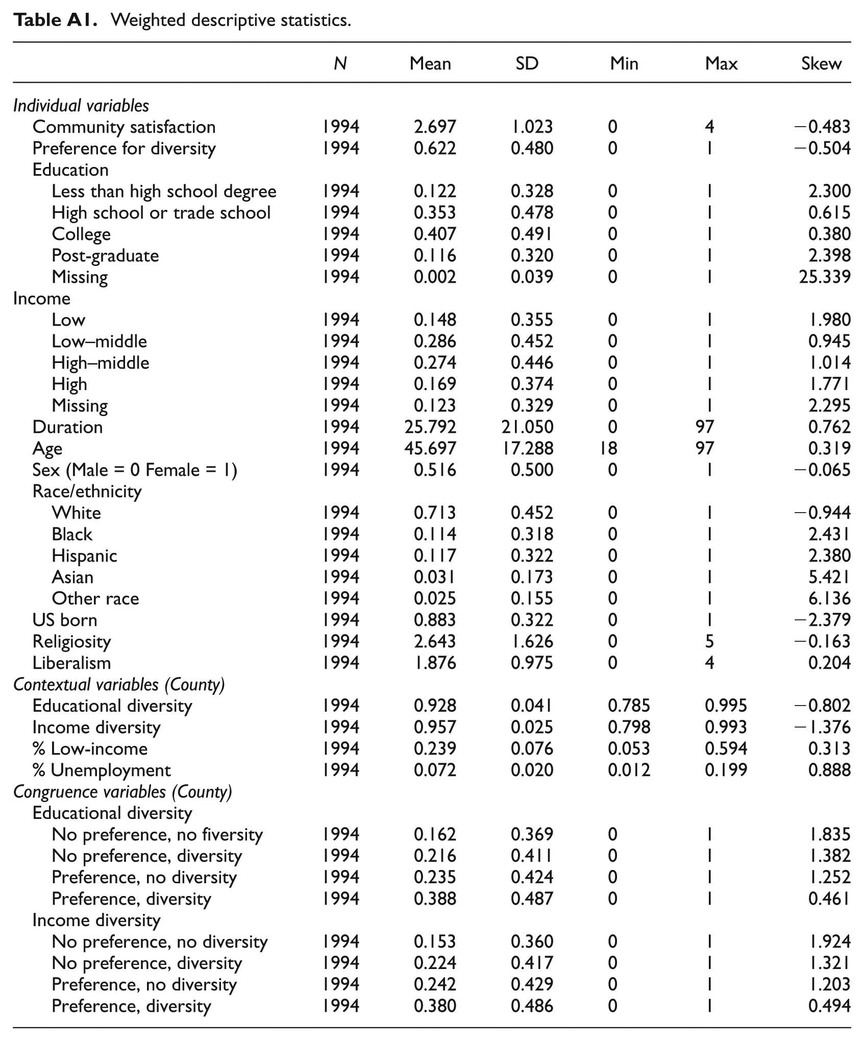
My study includes a range of control variables previously shown to be correlated with preference for diversity and community satisfaction (Campbell et al., 1976; Connerly and Marans, 1985; Galster and Hesser, 1981; Lu, 1999; Mohan and Twigg, 2007). Theses control variables are also generated from the Pew Social Trends survey. Duration is a continuous variable, which measures the proportion of lifetime years a respondent has lived in the local community. It is calculated by dividing years spent in local community by age. Age is a continuous variable ranging from 18 to 97 or over. Sex is a dummy variable, with a value of 1 indicating that the respondent is female. Race/ethnicity is reported using five mutually exclusive and exhaustive dummy variables: non-Hispanic white, non-Hispanic black, Hispanic, non-Hispanic Asian and other or mixed-race. Nativity is indicated with the variable U.S. Born; a score of one indicates that the respondent was born in the USA. Religiosity is measured on a five-point scale where a score of zero indicates that the respondent never attends religious services and a score of five indicates that the respondent attends religious services more than once a week. The variable liberalism expresses the respondent’s political ideology on a five-point scale ranging from very conservative at the low end to very liberal at the high end. Both the religiosity and liberalism variables reflect beliefs that may shape the interpretive process underlying satisfaction, the likelihood of taking action to improve community conditions and an individual’s general outlook on life. All of the individual control variables have less than 6% missing data. In order to maintain a consistent sample throughout the analysis, list-wise deletion was employed with the exceptions already noted for income and education. Weighted summary statistics for the resulting sample of 1994 are presented in the Appendix in Table A1.

The Pew Social Trends survey permits the exploration of the residential context of respondents since it includes the county of residence for each respondent. This study uses the 2005–2009 American Community Survey (ACS) five-year estimates to generate socioeconomic variables for each respondent’s county of residence. The ACS provides data annually for a sample of the US population. I utilise the 2005–2009 estimates because the time period straddles the Pew survey collection and because the five-year estimates include data for all counties and are more reliable than single- or three-year estimates.

In order to reflect the socioeconomic context of respondents’ communities, I create a series of socioeconomic variables. Diversity measures are calculated for education and income. Diversity is quantified using a score on the entropy index (E) for the county, which I have standardised by dividing by the natural log of the number of unique groups. The equation for the standardised entropy index, where π_r equals an educational or income category’s proportion of the county population, is (Iceland, 2004):

E = \sum_{r = 1}^{r} (π_{r}) \ln [\frac{1}{π_{r}}]

(1)

Quantified this way, diversity indicates how evenly the different socioeconomic groups are represented within the community. The measure can range from 0 to 1, with a score of 1 equalling perfect diversity, where all groups are represented evenly (i.e. make up the same proportion of the population), and a score of 0 equalling perfect homogeneity, where only one group is present.

Five educational attainment groups for the county population 25 years and over are used to construct the educational diversity measure: no high school degree; high school degree; some college; four-year college degree; and master’s, professional or doctorate degree. Income diversity reveals the county distribution of the following eight household income categories: less than US$10,000; US$10,000 to less than US$25,000; US$25,000 to less than US$40,000; US$40,000 to less than US$60,000; US$60,000 to less than US$75,000; US$75,000 to less than US$100,000; US$100,000 to less than US$150,000; and US$150,000 or more.

Some scholars have suggested that the concentration of certain income groups is more important than socioeconomic diversity (Baum et al., 2010). In order to explore this possibility, I consider percent low-income in the analysis. Households are considered low-income if they earn less than US$25,000, which translates to approximately 50% of the national median household income (Galster et al., 2008). The last contextual socioeconomic measure is percent unemployment, which indicates the percentage of the civilian population 16 years and over that is in the labour force but is not employed. Weighted descriptive statistics for the contextual variables are presented in the Appendix in Table A1.

Finally, I combine individual and contextual data to create socioeconomic diversity congruence variables. The congruence variables indicate whether respondents’ preferences for diversity align with the diversity of their communities. For each type of socioeconomic diversity there are four dummy variables: no preference – no diversity; no preference – diversity; preference – no diversity; and preference – diversity. In the first and the last groups, congruence is achieved because preferences and experiences match.

A county is considered diverse if its diversity is higher than the mean diversity of all areas in the study. According to this criterion, 58% of respondents live in counties that are educationally diverse and 59% live in counties that have high income diversity. Weighted descriptive statistics for the congruence variables (presented in the Appendix in Table A1) reveal that diversity preferences and experiences align for only slightly more than half of respondents.

Data analysis

The analysis begins with an examination of two antecedents of satisfaction: preferences and experiences. Specifically, I consider the relationships among individual socioeconomic and control variables, preferences for diversity and actual diversity. As an initial step, I employ weighted logistic regression to assess how respondents’ education and income, duration, age, sex, race/ethnicity, nativity, religiosity and political ideology relate to their preferences for socioeconomic diversity. I then use weighted ordinary least squares (OLS) regression to evaluate how the same individual characteristics, as well as diversity preference, relate to living in communities with high educational and income diversity, respectively.

The second part of the analysis looks at respondents’ reports of community satisfaction directly. I employ weighted OLS regression to assess how individual socioeconomic and control variables relate to community satisfaction. Next, I add contextual socioeconomic variables to the equation and regress community satisfaction on individual socioeconomic and control variables as well as educational diversity, income diversity, percent low-income and percent unemployment.

In the last set of models, I return to the idea of explaining satisfaction through the correspondence of preferences and experiences. I regress community satisfaction on education and income, individual control variables and socioeconomic diversity congruence measures. The weighted regression is run twice in order to test whether it matters which type of diversity is used (educational or income).

Since the analyses include individual as well as contextual variables, it is possible that clustering could influence the regression results. However, because of the sampling method there is minimum clustering within the data. More than half of the counties contain only one respondent and only 31 counties have 10 or more respondents. Still, in order to be conservative, I correct for clustering by using robust standard errors in all of the regressions.

Results

Socioeconomic diversity preference

Table 1 shows the results from the weighted logistic regression of preference for socioeconomic diversity on individual education, income and control variables. The reference group for education, in this and all other models, is high school degree or trade school. Compared with this group, having less than a high school degree decreases the odds of having a preference for diversity by 44% holding all other variables constant (see the odds ratios in the third column). Following the same trend, the odds of having a preference for socioeconomic diversity increases by 26% for those with some college or a college degree and by 44% for those with post-graduate training controlling for all other variables. In general, education is positively and statistically significantly related to preference for diversity. The only education group without a significant effect is the group for which education data are missing. In contrast, none of the income groups are statistically significantly related to preference for diversity. Several of the control variables show significant relationships with preference for diversity. Being US born and being more liberal both increase the odds of having a preference for socioeconomic diversity. Duration is also negatively related with preference for diversity. However, this relationship is only marginally significant (p = 0.058).

Table 1.

Weighted logistic regression of diversity preference on individual SE and control variables.

	β	Robust SE(β)	Odds ratio
Socioeconomic variables
Education
Less than H.S. degree	−0.572**	0.202	0.564
College	0.228*	0.113	1.257
Post-graduate	0.366*	0.170	1.442
Missing	−1.589	1.140	0.204
Income
Low	−0.094	0.204	0.911
High-middle	−0.086	0.136	0.918
High	0.151	0.169	1.163
Missing	0.341^†	0.179	1.406
Control variables
Duration	−0.003^†	0.002	0.997
Age	0.000	0.003	1.000
Female	−0.057	0.109	0.944
Race/ethnicity
Black	0.211	0.189	1.235
Hispanic	0.291	0.203	1.338
Asian	−0.052	0.365	0.949
Other race	0.634 ^†	0.385	1.885
US born	0.600**	0.202	1.822
Religiosity	0.056	0.035	1.057
Liberalism	0.176**	0.061	1.192
Constant	−0.478	0.321	0.620
χ²	59.97
d.f.	18.000
Pseudo R²	0.031

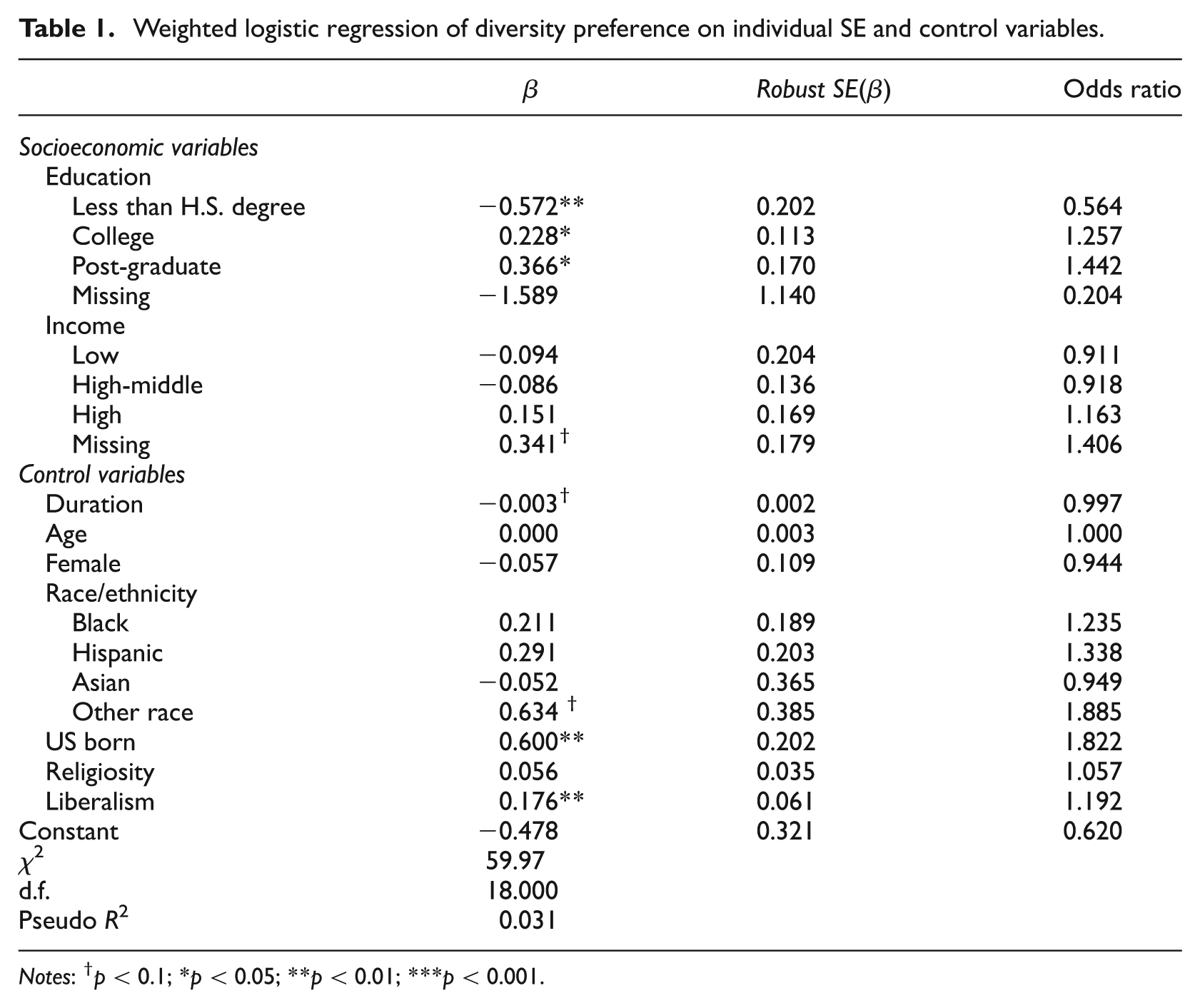
Notes: ^† p < 0.1; *p < 0.05; **p < 0.01; ***p < 0.001.

Correlates of community diversity

Who is most likely to live in communities that have high levels of socioeconomic diversity? Table 2 illustrates the results of two weighted OLS regressions of county-level socioeconomic diversity on individual socioeconomic and control variables. In the first model, socioeconomic diversity is measured using educational diversity and in the second model it is measured using income diversity.

Table 2.

Weighted OLS regression of community diversity on individual variables.

	Educational diversity		Income diversity
	b	Robust SE	b	Robust SE
Socioeconomic variables
Education
Less than H.S. degree	−0.005	0.004	−0.004	0.003
College	0.009***	0.002	0.004*	0.002
Post-graduate	0.014***	0.003	0.006***	0.002
Missing	0.027**	0.008	0.017***	0.005
Income
Low	0.005	0.004	0.003	0.002
High-middle	0.006*	0.003	0.002	0.002
High	0.015***	0.003	0.007***	0.002
Missing	0.011**	0.004	0.005*	0.002
Diversity preference	0.003	0.002	0.001	0.001
Control variables
Duration	−0.000**	0.000	−0.000*	0.000
Age	0.000	0.000	0.000	0.000
Female	0.000	0.002	0.000	0.001
Race/ethnicity
Black	0.021***	0.003	0.006**	0.002
Hispanic	0.015**	0.004	0.006*	0.003
Asian	0.018***	0.005	0.005	0.005
Other race	−0.001	0.008	0.002	0.003
US born	−0.013***	0.003	−0.004*	0.002
Religiosity	−0.002**	0.001	−0.002***	0.000
Liberalism	0.003**	0.001	0.001	0.001
Constant	0.925***	0.006	0.957***	0.004
R ²	0.127		0.064
F-Statistic	12.40		6.40

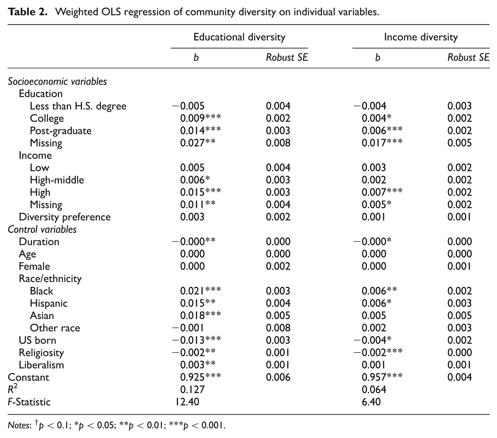
Notes: ^† p < 0.1; *p < 0.05; **p < 0.01; ***p < 0.001.

In both models, education and income are positively related to community diversity. Having more income and a higher education is associated with living in a county with higher levels of educational and income diversity.

Interestingly, the coefficient for the missing income group is statistically significant in both models. This suggests that data for income are not missing at random, but that people who decline to report their incomes may differ from the rest of the sample in a meaningful way. The coefficients for this group are most similar to the high income group, which supports the commonly held belief that people with higher incomes are less likely to report their incomes. The last socioeconomic predictor, preference for diversity, is not significant in either model indicating a lack of correspondence between preferred and actual (objective) diversity.

No matter which measure of socioeconomic diversity is employed, education or income, the relationships between the individual control variables and community diversity remain largely unchanged. In both models, being a racial/ethnic minority, being foreign born and being liberal are positively related to living in a socioeconomically diverse county. In contrast, controlling for all other variables, duration and higher religiosity are negatively related to residing in a diverse community.

While the general patterns are the same between the two models, the individual socioeconomic and control variables explain more of the variance in educational diversity (12.7%) than in income diversity (6.4%). In addition, the coefficients are stronger and the significance levels are higher in the educational diversity model than in the income diversity model.

Accounting for variation in satisfaction

What role does socioeconomic status play in residents’ satisfaction with their communities? In the first model of Table 3, community satisfaction is regressed on three individual socioeconomic variables (education, income and diversity preference) as well as individual control variables. The model explains 10.5% of the variance in community satisfaction. Education is positively related to satisfaction; however, post-graduate is the only group with a statistically significant coefficient. Income is also positively and significantly related to satisfaction. Respondents with higher levels of income report higher levels of community satisfaction. Diversity preference, once again, is not statistically significant. Among the control variables, being black or Asian versus white is negatively related to satisfaction.

Table 3.

Weighted OLS regression of community satisfaction on individual and contextual variables.

	Individual		Individual + contextual
	b	Robust SE	b	Robust SE
Individual SE variables
Education
Less than H.S. degree	−0.098	0.101	−0.091	0.101
College	0.103^†	0.060	0.098^†	0.059
Post-graduate	0.253**	0.080	0.233**	0.078
Missing	0.035	0.261	0.012	0.281
Income
Low	−0.221*	0.097	−0.213*	0.096
High-middle	0.142*	0.063	0.142*	0.063
High	0.292***	0.074	0.258***	0.073
Missing	0.072	0.086	0.074	0.085
Diversity preference	0.034	0.051	0.033	0.050
Individual control variables
Duration	−0.000	0.001	−0.000	0.001
Age	0.003^†	0.002	0.003^†	0.001
Female	0.043	0.049	0.045	0.048
Race/ethnicity
Black	−0.604***	0.094	−0.525***	0.093
Hispanic	−0.176^†	0.098	−0.150	0.100
Asian	−0.475*	0.198	−0.447*	0.187
Other race	−0.183	0.230	−0.145	0.222
US born	−0.002	0.106	−0.005	0.104
Religiosity	0.019	0.018	0.018	0.017
Liberalism	−0.046	0.029	−0.050^†	0.029
Contextual SE variables
Educational diversity			0.226	0.816
Income diversity			−1.022	1.252
% Low-income			−0.251	0.404
% Unemployment			−6.056***	1.437
Constant	2.562***	0.169	3.826***	1.028
R ²	0.105		0.121
F-Statistic	7.50		8.58

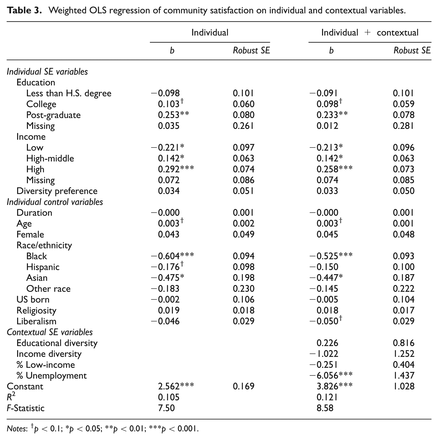
Notes: ^† p < 0.1; *p < 0.05; **p < 0.01; ***p < 0.001.

In the second model in Table 3, contextual county-level socioeconomic variables are added to the analysis. Adding contextual socioeconomic variables to the weighted OLS regression model increases the explained variance to 12.1%. While educational diversity, income diversity and percent low-income all lack significance, percent unemployment has a statistically significant, negative relationship with community satisfaction. When more people in the community are unemployed, respondents are less satisfied.

Does congruence matter?

In a final set of models, I test to what extent the congruence between preferences for and experiences with diversity can explain variations in community satisfaction. The results from these models are displayed in Table 4. The relationships between individual education and income and community satisfaction are consistent with those found in previous models. The same is true for the individual control variables. However, none of the congruence variables are statistically significant, suggesting that congruence between preferences and experiences with community does not have an effect on community satisfaction.

Table 4.

Weighted OLS regression of community satisfaction on individual and diversity congruence variables.

	Educational diversity		Income diversity
	b	Robust SE	b	Robust SE
Individual SE + control
Education
Less than H.S.	−0.097	0.101	−0.097	0.102
College	0.098	0.060	0.102	0.060
Post-graduate	0.248**	0.080	0.250**	0.080
Missing	0.007	0.264	0.041	0.360
Income
Low	−0.223*	0.098	−0.223*	0.098
High-middle	0.138*	0.064	0.140*	0.063
High	0.287***	0.074	0.290***	0.073
Missing	0.066	0.086	0.070	0.086
Duration	−0.000	0.001	−0.000	0.001
Age	0.002	0.002	0.003^†	0.002
Female	0.045	0.049	0.041	0.049
Race/ethnicity
Black	−0.616***	0.094	−0.605***	0.095
Hispanic	−0.181^†	0.100	−0.178^†	0.099
Asian	−0.480*	0.199	−0.478*	0.199
Other race	−0.189	0.228	−0.180	0.229
US born	0.009	0.106	0.001	0.105
Religiosity	0.020	0.018	0.019^†	0.018
Liberalism	−0.045	0.029	−0.047*	0.029
Diversity congruence
No preference, diversity	0.109	0.078	0.030	0.079
Preference, no diversity	0.136	0.090	−0.032	0.090
Preference, diversity	0.118	0.081	−0.006	0.082
Constant	2.479***	0.178	2.584***	0.177
R ²	0.107		0.106
F-Statistic	7.06		6.91

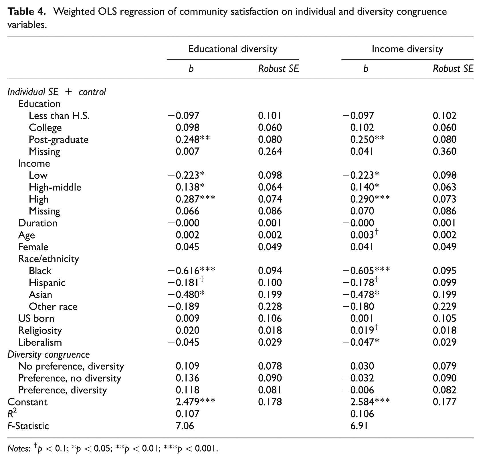
Notes: ^† p < 0.1; *p < 0.05; **p < 0.01; ***p < 0.001.

Discussion

Community satisfaction is important for individuals, communities and the nation as a whole. Because of its effect on quality of life, its impact on community vitality and its primacy in government policies and assessments, community satisfaction should maintain an important place in scholars’ research agendas. There is still much we do not understand about the relationships among socioeconomic status, preferences and community satisfaction.

This study takes a first step toward unravelling some of these relationships by examining both individual and contextual socioeconomic status, including socioeconomic diversity, and by considering two antecedents of satisfaction: preferences and experiences. Consistent with previous studies, I find that higher socioeconomic status, in the form of education, is associated with having a preference for socioeconomic diversity. In addition, US born respondents and those who report higher levels of liberalism are more likely to prefer socioeconomic diversity. Community planners could use this information on preferences for diversity to recruit residents for mixed-income housing developments.

However, in the USA, class and race are intricately related, so it is possible that when a respondent expresses an attitude toward socioeconomic diversity, they could really be expressing an attitude toward racial/ethnic diversity. Additional analyses were estimated in order to consider the possibility that preference for socioeconomic diversity was merely a euphemism for preference for racial/ethnic diversity. However, preference for racial/ethnic diversity and preference for socioeconomic diversity were only weakly correlated (r = 0.212) and controlling for preference for racial/ethnic diversity, the results in Table 2 and Table 3 remain the same. Still, it is possible that social desirability bias could be affecting these results. It may no longer be socially acceptable to report an aversion to living in close proximity to racial/ethnic minorities, but respondents may feel more comfortable reporting an aversion to living near lower-income residents. In a country where race is highly correlated with income, completely separating socioeconomic diversity from racial/ethnic diversity may never be possible.

This study confirms that preferences do not always align with experiences. My results show that having a preference for diversity is not significantly related to living in a more socioeconomically diverse community. Still, socioeconomic status seems to influence experiences with diversity. When socioeconomic diversity is operationalised as educational or income diversity, having more education and income is positively associated with living in a diverse community. This could be because higher socioeconomic status provides more opportunity to live in different types of neighbourhoods, including ones that are socioeconomically diverse. Lower-income individuals and those with little education may be trapped in lower-income, relatively homogeneous communities. Control variables such as duration, racial/ethnic minority status, political liberalism and religiosity are also strong predictors of socioeconomic diversity.

My study consistently demonstrates that individual socioeconomic variables influence community satisfaction. Individual education and income explain a non-trivial proportion of the variation in satisfaction and remain statistically significant after controlling for age, gender, race/ethnicity, religiosity, political ideology and contextual socioeconomic variables. This may be because people with higher income and more education live in physically nicer communities with more amenities, or because they feel that they have more control over their life and their surroundings. Among the contextual socioeconomic variables, percent unemployment is the strongest predictor of dissatisfaction. Such a finding hints that poverty and other social problems related to unemployment might be important for community satisfaction. However, since I was not able to include individual unemployment in my models, it is also possible that percent unemployment could be capturing an individual effect of personal unemployment on community satisfaction. Essentially, in a community with a high unemployment rate, the likelihood that any individual is unemployed is increased. Future research should examine the relationship between individual unemployment and community satisfaction.

The lack of alignment between preferences for and experiences with socioeconomic diversity is interesting, and one might posit that it would have a negative effect on community satisfaction. However, my analyses reveal that neither preferences for diversity nor contextual socioeconomic diversity are significantly related to community satisfaction. Furthermore, when diversity congruence variables are considered, respondents whose preferences and experiences with diversity align are no more likely to be satisfied with their communities.

While the insignificance of the congruence variable is surprising, it is possible that congruence between preferences and experiences with regard to some other contextual attribute, such as quality of schools or public transportation, could be more important for community satisfaction. Future research that considers residents’ preferences or expectations for different community characteristics could add to the community satisfaction literature.

Since my analyses rely on survey data I am also limited by the quality of responses. The response rate of 22% could have influenced my results. In addition, I am limited by the geographic identifiers that are available to me. The county has merit as a community unit because of its role as a governing unit and in many cases aligns well with the size of a typical community. However, some counties may be too large to capture the concept of community well. Future studies should employ different geographic units. In particular, I think that smaller geographic units, such as census places or towns, would be an appropriate size. Including contextual community measures is a first step toward understanding the antecedents of community satisfaction; however, by ignoring aspirations, current studies of satisfaction are leaving out half of the picture.

Footnotes

Appendix

Table A1.

Weighted descriptive statistics.

	N	Mean	SD	Min	Max	Skew
Individual variables
Community satisfaction	1994	2.697	1.023	0	4	−0.483
Preference for diversity	1994	0.622	0.480	0	1	−0.504
Education
Less than high school degree	1994	0.122	0.328	0	1	2.300
High school or trade school	1994	0.353	0.478	0	1	0.615
College	1994	0.407	0.491	0	1	0.380
Post-graduate	1994	0.116	0.320	0	1	2.398
Missing	1994	0.002	0.039	0	1	25.339
Income
Low	1994	0.148	0.355	0	1	1.980
Low–middle	1994	0.286	0.452	0	1	0.945
High–middle	1994	0.274	0.446	0	1	1.014
High	1994	0.169	0.374	0	1	1.771
Missing	1994	0.123	0.329	0	1	2.295
Duration	1994	25.792	21.050	0	97	0.762
Age	1994	45.697	17.288	18	97	0.319
Sex (Male = 0 Female = 1)	1994	0.516	0.500	0	1	−0.065
Race/ethnicity
White	1994	0.713	0.452	0	1	−0.944
Black	1994	0.114	0.318	0	1	2.431
Hispanic	1994	0.117	0.322	0	1	2.380
Asian	1994	0.031	0.173	0	1	5.421
Other race	1994	0.025	0.155	0	1	6.136
US born	1994	0.883	0.322	0	1	−2.379
Religiosity	1994	2.643	1.626	0	5	−0.163
Liberalism	1994	1.876	0.975	0	4	0.204
Contextual variables (County)
Educational diversity	1994	0.928	0.041	0.785	0.995	−0.802
Income diversity	1994	0.957	0.025	0.798	0.993	−1.376
% Low-income	1994	0.239	0.076	0.053	0.594	0.313
% Unemployment	1994	0.072	0.020	0.012	0.199	0.888
Congruence variables (County)
Educational diversity
No preference, no fiversity	1994	0.162	0.369	0	1	1.835
No preference, diversity	1994	0.216	0.411	0	1	1.382
Preference, no diversity	1994	0.235	0.424	0	1	1.252
Preference, diversity	1994	0.388	0.487	0	1	0.461
Income diversity
No preference, no diversity	1994	0.153	0.360	0	1	1.924
No preference, diversity	1994	0.224	0.417	0	1	1.321
Preference, no diversity	1994	0.242	0.429	0	1	1.203
Preference, diversity	1994	0.380	0.486	0	1	0.494

Acknowledgements

The author would like to thank Barrett A Lee, Marin R Wenger, Michael Timberlake and anonymous referees for their support and helpful comments.

Funding

Support for this research has been provided by a National Science Foundation Graduate Research Fellowship (DGE1255832) and from the Population Research Institute of Penn State University, which receives infrastructure funding from the Eunice Kennedy Shriver National Institute of Child Health and Human Development (R24HD041025). Any opinions, findings, and conclusions or recommendations expressed in this material are those of the author and do not necessarily reflect the views of the National Science Foundation or the National Institutes of Health.

References

Andersson

Musterd

Galster

. (2007) What mix matters? Exploring the relationships between individuals’ incomes and different measures of their neighborhood context. Housing Studies 22(5): 637–660.

Baum

Arthurson

Rickson

(2010) Happy people in mixed-up places: The association between the degree and type of local socioeconomic mix and expressions of neighborhood satisfaction. Urban Studies 47(3): 467–485.

Blokland

van Eijk

(2010) Do people who like diversity practice diversity in neighbourhood life? Neighbourhood use and the social networks of ‘diversity seekers’ in a mixed neighbourhood in the Netherlands. Journal of Ethnic and Migration Studies 36(2): 313–332.

Campbell

Converse

Rodgers

(1976) The Quality of American Life: Perceptions, Evaluations, and Satisfactions. New York: Russell Sage Foundation.

Chaskin

Joseph

(2010) Building ‘community’ in mixed-income developments: Assumptions, approaches, and early experiences. Urban Affairs Review 45(3): 299–335.

Connerly

Marans

(1985) Comparing two global measures of perceived neighborhood quality. Social Indicators Research 17: 29–47.

Durband

Eckart

(1973) Social rank, residential effects and community satisfaction. Social Forces 52(1): 74–85.

Filkins

Allen

Cordes

(2000) Predicting community satisfaction among rural residents: An integrative model. Rural Sociology 65(1): 72–86.

Fried

(1982) Residential attachment: Sources of residential and community satisfaction. Journal of Social Issues 38(3): 107–119.

10.

Fried

(1986) The neighborhood in metropolitan life: Its psychosocial significance. In: Taylor

(ed.) Urban Neighborhoods: Research and Policy. New York: Praeger Publishers, pp. 331–336.

11.

Galster

Hesser

(1981) Residential satisfaction: Compositional and contextual correlates. Environment and Behavior 13(6): 735–758.

12.

Galster

Andersson

Musterd

(2010) Who is affected by neighbourhood income mix? Gender, age, family, employment and income differences. Urban Studies 47(14): 2915–2944.

13.

Galster

Booza

Cutsinger

(2008) Income diversity within neighborhoods and very low-income families. Cityscape: A Journal of Policy Development and Research 10(2): 257–300.

14.

Goudy

(1977) Evaluations of local attributes and community satisfaction in small towns. Rural Sociology 42(3): 371–382.

15.

Grinstein-Weiss

Yeo

Anacker

. (2011) Homeownership and neighborhood satisfaction among low- and moderate-income households. Journal of Urban Affairs 33(3): 247–265.

16.

Heaton

Fredrickson

Fuguitt

. (1979) Residential preferences, community satisfaction, and the intention to move. Demography 16(4): 565–573.

17.

Hipp

(2009) Specifying the determinants of neighborhood satisfaction: A robust assessment in 24 metropolitan areas. Social Forces 88(1): 395–424.

18.

Iceland

(2004) The Multigroup Entropy Index (Also Known as Theil’s H or the Information Theory Index). US Census Bureau. Available at: http://www.census.gov/hhes/www/housing/housing_patterns/multigroup_entrpy.pdf (accessed 20 January 2011).

19.

Lee

Guest

(1983) Determinants of neighborhood satisfaction: A metropolitan-level analysis. The Sociological Quarterly 24(2): 287–303.

20.

(1999) Determinants of residential satisfaction: Ordered logit vs. regression models. Growth and Change 30: 264–897.

21.

McKinnish

White

(2011) Who moves to mixed-income neighborhoods? Regional Science and Urban Economics 41(3): 187–195.

22.

Miller

Tsemberis

Malia

. (1980) Neighborhood satisfaction among urban dwellers. Journal of Social Issues 36: 101–117.

23.

Mohan

Twigg

(2007) Sense of place, quality of life and local socioeconomic context: Evidence from the Survey of English Housing, 2002/03. Urban Studies 44(10): 2029–2945.

24.

Musterd

(2008) Residents’ views on social mix: Social mix, social networks and stigmatisation in post-war housing estates in Europe. Urban Studies 45(4): 897–915.

25.

Parkes

Kearns

Atkinson

(2002) What makes people dissatisfied with their neighbourhoods? Urban Studies 39(13): 2413–2438.

26.

Permentier

Bolt

van Ham

(2011) Determinants of neighbourhood satisfaction and perception of neighbourhood reputation. Urban Studies 48(5): 977–996.

27.

Pew Research Center (2009) Methodology: Pew Social Trends – October 2008. Available at: http://pewsocialtrends.org/category/datasets/?download=900 (accessed 1 March 2011).

28.

Putnam

(2007) E pluribus unum: Diversity and community in the twenty-first century: The 2006 Johan Skytte Prize Lecture. Scandinavian Political Studies 30(2): 137–174.

29.

Sarkissian

(1976) The idea of social mix in town planning: An historical review. Urban Studies 13: 231–246.

30.

Stipak

Hensler

(1983) Effect of neighborhood racial and socioeconomic composition on urban residents’ evaluations of their neighborhoods. Social Indicators Research 12(3): 331–320.

31.

Talen

(2010) The context of diversity: A study of six Chicago neighborhoods. Urban Studies 47(3): 486–513.

32.

Theodori

(2001) Examining the effects of community satisfaction and attachment on individual well-being. Rural Sociology 66(4): 618–628.

33.

Turner

(1997) Achieving a new urban diversity: What have we learned? Housing Policy Debate 8(2): 295–305.