
Abstract
Social scientists have long studied the effects of cities on human wellbeing and happiness. This article demonstrates that people in cities are less happy, confirming a long-standing argument in the literature. But it had not yet been tested whether it is urbanism that negatively affects happiness, or if urban problems such as crime and poverty are to blame. Wirth posited that urbanism itself led to negative effects, but Fischer noted the necessity of empirical tests of Wirth’s ideas. This study uses a happiness measure to provide a new look at the old question of urban unhappiness. Using the Behavioral Risk Factor Surveillance System from the US Centers for Disease Control and Prevention, we aim to untangle the effects of the city itself and urban problems on happiness in the USA. We find that the core characteristics of urban life (in particular size and density) contribute to urban unhappiness, controlling for urban problems. Urban unhappiness persists regardless of urban characteristics.
This article addresses a fundamental social science question: how does the modern world affect those who live in it? Modernisation and industrialisation brought urbanisation, rife with complex problems. Tönnies ([1887] 2002) and Durkheim ([1893] 1997) challenged us to investigate what living in cities does to us. The first American sociologists, Louis Wirth among them, were urban sociologists, similarly concerned with city characteristics, urban problems and happiness (Wirth, 1938). They did not use the term happiness, but other terms to denote the negative side of the urban way of life, such as ‘malaise’. 1 Wirth’s theory of urban life focused on how urbanism led to various negative consequences, including (1) cognitively, in terms of alienation, (2) behaviourally, in terms of deviance, and (3) structurally, in terms of anomie (normlessness), all of which would lead to unhappiness.
There is a long-standing debate about whether people in cities are unhappy. The academic debate started in sociology (Durkheim, [1893] 1997; Park, 1915; Weber et al., [1921] 1962; Wirth, 1938), but was abandoned by sociologists in the 1970s after Fischer’s major works were published. Recently, the topic was taken up by other disciplines, yet it has not addressed sociological research, and has used other approaches and foci. Regardless of the fact that urban life has much to offer residents, there is a consensus emerging among scholars that city living makes us, on average, unhappy and unhealthy (Adams, 1992; Adams and Serpe, 2000; Amato and Zuo, 1992; Balducci and Checchi, 2009; Berry and Okulicz-Kozaryn, 2009, 2011; Evans, 2009; Lederbogen et al., 2011). Those authors, however, used small data sets with few variables, typically operationalised city simply as the size of settlement, or used a dichotomous urban/rural variable. No study has controlled for city-level variables such as per capita income; no study so far has used a model that accounts for both personal and city-level factors that affect happiness. A fundamental question as framed by Fischer (1972, 1973, 1975) remains unanswered: is it cities themselves, in terms of size, density, and heterogeneity, that lead to unhappiness, or is it problems people typically associate with cities – notably poverty, crime and lack of support – that make people unhappy?
The first urban sociologists proposed that urbanisation created malaise (unhappiness) because of the core characteristics of cities: increased population size created anonymity and impersonality, density created sensory overload and withdrawal from social life, and heterogeneity led to anomie and deviance (see Park et al., [1925] 1984; Simmel, 1903; Tönnies [1887] 2002; Wirth, 1938). Some might assert that cities are defined by their problems, and argue that measures can be used interchangeably to examine both urbanism and urban problems. However, we follow Park, Wirth, and others to define urbanism by using population size and density. We seek to advance the understanding of urban unhappiness by better measuring urbanism using several size and density variables, and controlling for urban characteristics and problems to test whether urban unhappiness persists regardless of them. Recent large-scale survey data representative of a wide range of cities, as well as counties that are not cities as a comparison group, make this test possible.
Theoretical background
There are many advantages to cities. Labour specialisation, economies of scale, invention and creativity are all made possible by high-density living (e.g. Florida, 2008; Glaeser, 2011; O’Sullivan, 2009). Human civilisation as we know it was made possible by cities and the labour specialisation that took place in them (O’Sullivan, 2009); this made organic solidarity possible (Durkheim, [1893] 1997). Average standard of living has improved tremendously, even with high levels of inequality: by one estimate, those in the bottom decile today have a better standard of living than all but the top 1% did 100 years ago (Bok, 2010). For an overview of the progress that Americans have made since colonial times, see Fischer (2010). Progress in standard of living and urbanisation are closely related, leading some scholars to conclude that we are happier in cities than we are elsewhere (Glaeser, 2011); this is not so. In fact, Americans have not become any happier over time (Easterlin, 1974), and we are, on average, the least happy in cities (Berry and Okulicz-Kozaryn, 2011). The most celebrated thinkers in America’s intellectual history almost universally expressed ambivalence or animosity toward the city, among them: Jefferson, Emerson and Thoreau (White and White, 1977). Wirth (1938) famously summarised the negatives of city life, building on the worries of earlier European sociological theories (Tönnies, [1887] 2002). Cities are collections of heterogeneous people with different specialisations; there is a lot of variability among city dwellers. Relations between them are anonymous, superficial, impersonal, transitory, unstable and insecure (Wirth, 1938). Early theorists lamented what they saw as a lack of norms, which led to moral deviance such as crime (Wirth, 1938). Cities are fast-paced and crowded, creating a psychological overload because of the intensification of stimuli for urban dwellers and occasioning detachment, and a retreat to social isolation (Simmel, 1903). Simmel argued that people necessarily adapted to urban life by developing a blasé attitude: with the rapid pace and all the people we come across, we would not be able to handle it if we had to deeply engage with everyone and everything, so we become detached. Simmel noted that this reserve provides more personal freedom and privacy to urban dwellers, but it also necessitates impersonal interactions with those we encounter (Simmel, 1903). Cities generate moral disorder: misunderstandings, tension and conflict (Smelser and Alexander, 1999). For more elaboration see Fischer and Merton (1976).
Recent evidence raises other concerns about cities: density and heterogeneity predict lower social capital (Helliwell and Wang, 2010) and low social capital is associated with poor health and higher mortality (Kawachi et al., 1997; Subramanian et al., 2002). Poverty is concentrated in cities, and the more concentrated the poverty, the worse it is for people (Jargowsky, 1997). There is an abundance of crime (Bettencourt et al., 2007, 2010) and segregation (Jargowsky, 1997; Massey and Denton, 1993). There is more crime in cities than there is elsewhere, and high crime predicts poor health (Lynch et al., 2004; Zimmerman and Bell, 2006).
High density predicts low happiness (Fassio et al., 2013; Lawless and Lucas, 2011). One specific reason why there may be less happiness in cities is that ‘the pecuniary nexus tends to displace personal relations’ (Wirth, 1938: 1). In addition, ‘fashion tends to take the place of custom’ (Park, 1915: 605), and consumption does not have a lasting impact on life satisfaction because people adapt to material goods (Easterlin, 2003). Recent neurological evidence confirms early sociological theory: great cities actually overstimulate our brains to the point where it is not healthy (Lederbogen et al., 2011). Schwartz (2004) shows that the abundance of choice, exemplified in cities, often leads to depression, loneliness, anxiety and stress. Americans do not merely prefer smaller areas as documented earlier by Fuguitt and Zuiches (1975) and Fuguitt and Brown (1990), they are also happier in smaller areas (Lawless and Lucas, 2011).
There have been many attempts at discerning the effect of city living on happiness. But the limitation of even the most recent research is that it does not control for city-level variables such as per capita income, and city disadvantages such as crime and poverty, something that Fischer suggested researchers should do over 40 years ago. Fischer (1973: 222) acknowledged that people are less happy in the biggest cities, but he was not sure whether it was urbanism or other confounding variables that make residents unhappy in cities:
(1) Such preferences [for rural living] may be a function of idealized images founded on popular conceptions of urban and rural life. (2) They may indicate utopian hopes of maintaining urban opportunities in small communities. […] (3) These evaluations may result from the contemporary state of American cities rather than from the nature of cities per se.
The remainder of this article will try to answer item (3) above. We aim to discover whether city residents are less happy, controlling for problems people typically associate with contemporary cities. If so, these problems cannot be the cause of lower happiness in cities. Rather, urbanism’s core characteristics – large numbers of people and high density – along with other factors, make city dwellers unhappy:
H1: people in cities are less happy than are those in other areas if cities are defined by:
H1a: population size
H1b: density
H2: urban unhappiness will persist after controlling for problems people typically associate with cities.
In testing the above hypotheses we control for city characteristics that may affect happiness and for known person-level predictors of happiness.
Data and measurement
We analyse the 2005 Behavioral Risk Factor Surveillance System (BRFSS) from the United States Centers for Disease Control and Prevention. The BRFSS is representative of the USA, with a total sample size of over 100,000 people per year, well suited for the study of cities. The regular BRFSS data set, however, is not representative of most counties, so we use the SMART (Selected Metropolitan/Micropolitan Area Risk Trends) version of the BRFSS that is representative of counties; for simplicity we will refer to it as the BRFSS. The downside of the SMART version is a smaller number of counties, 232, but it still provides a good sample of the USA with enough variation. 2 See the appendix (available online) for a listing of counties. In addition to the 2005 BRFSS, as a robustness check, we include models using data for 2006, 2007 and 2008 in the appendix (available online), because the more recent waves have bigger samples, and to account for potential lag effects from variables measuring urban problems at the county level. In the main text we report the 2005 BRFSS results, because the county-level data we use are either for 2003, 2004 or 2005. All county-level data come from the Inter-university Consortium for Political and Social Research: County Characteristics, 2000–2007.
We use data at person and county levels. We do not have data at the city level. City attributes are measured at the county level; many metropolitan areas cover the whole county. Even where a metropolitan area covers part of a county, it seldom ends abruptly and changes into a non-urban area or open land. Where a metropolitan area abruptly ends, then it is due to a natural boundary such as an ocean in the case of coastal cities, but in that case the county ends as well. Furthermore, this limitation is ameliorated by another operationalisation of cities: the urban–rural continuum, which differentiates between metropolitan areas, cities, towns of various sizes and smaller areas. Another triangulation of measurement is performed using a person-level location variable: metropolitan status code.
The person-level dependent variable: Happiness
As noted above, we treat malaise as unhappiness, following research by Fischer (1972, 1973), who pioneered using happiness data to study urban malaise. Yet data and statistical software did not enable a proper test in the early 1970s. We use large-scale data and a model controlling for both personal and ecological characteristics.
Happiness is a multidimensional concept (e.g. Hills and Argyle, 2001), though for simplicity we use the terms happiness, life satisfaction and subjective wellbeing interchangeably (the dimensions overlap). The BRFSS has only one survey item measuring happiness. 3
The survey item reads ‘In general, how satisfied are you with your life?’. For simplicity, we recoded answers so that a higher numeric value means more happiness: 1 is ‘very dissatisfied’, 2 ‘dissatisfied’, 3 ‘satisfied’ and 4 ‘very satisfied’. Over 90% of respondents were either satisfied or very satisfied with their lives. The same variable has been used in recent happiness studies by Oswald and Wu (2010, 2011), Glaeser et al. (2014) and Winters and Li (2015).
The happiness measure, even though self-reported and subjective, is reliable, valid (Myers, 2000), and closely correlates with similar, more objective measures such as brain waves (Layard, 2005). Unhappiness strongly correlates with suicide incidence and mental health problems (Bray and Gunnell, 2006). Finally, to be clear, we study here general/overall happiness, not a domain-specific happiness such as neighbourhood or community satisfaction.
The main person- and county-level independent variables: City size/city population
In this study, we sacrifice breadth of measurement of urbanism at the cost of precision and use the most precise measures available: population size and density. Population size is used in two ways: as an urban–rural continuum with nine categories defined by the USDA (US Department of Agriculture) and as a metropolitan status code based on a survey item from the BRFSS. We chose continuous/ordinal measures because they convey more information than do binary or nominal ones (see Meyer, 2013; Wirth, 1938). The county-level urban–rural continuum ranges from 1 (‘metro>1 million’) to 9 (‘non-metro<2500, not adjacent to metro’). 4
The metropolitan status code differs within a county; it is a person-level variable and reflects the urban dweller status more precisely than does the county-level urban–rural continuum. The metropolitan status code is broken down into the following dummy variables: ‘not in an MSA’, ‘inside a suburban county of the MSA’ and ‘outside centre OR in MSA without centre’. ‘Centre city of MSA’ is the base case, and MSA stands for Metropolitan Statistical Area, a geographical area associated with an urban area of 50,000 people or more, as defined by the United States Office of Management and Budget.
The main county-level independent variable: Population density
We measure density as population (in thousands) per square mile, and there are staggering differences; density ranges from four people per square mile in Sweetwater County, WY to 70,000 people per square mile in New York County, NY.
The measures of urbanism we use do not capture heterogeneity directly. We do not include heterogeneity for three reasons. First, it is not obvious which type of heterogeneity is to be measured. In modern times we think of racial, ethnic and class diversity, but in Wirth’s conception, influenced by Durkheim’s focus on the increasing division of labour and occupational specialisation that accompanied urbanisation, heterogeneity may have been more about occupational diversity; Wirth writes of heterogeneity in ‘social groups’ (1938). It also may have been more about diversity in nation of origin, which while related to contemporary understandings of ethnicity, is not synonymous with the latter. As Wilson (2012) and Finney and Simpson (2005) note, sometimes the focus on race and ethnicity is misplaced. So we might consider measures of ethnicity or national origin, race, religion, income or occupation, for example. Second, there is precedent in recent literature to omit heterogeneity as part of a definition of urbanism, though literature consistently considers size and density (e.g. Meyer, 2013). Third, we looked at various measures of racial diversity, but did not find a consistent and robust relationship.
County-level controls: Measures of urban characteristics
As we have argued above, this paper’s key contribution is to disentangle the effects of the city (size, density) and urban problems on the happiness of city residents. To achieve that, we control for the following city characteristics: crime, housing stress, low education, low employment, persistent poverty, population loss, personal income (USD 1000)/cap, and percent Black. This set of controls addresses a fundamental confounding factor and an alternative explanation for city unhappiness: there are many poor people either stuck because they cannot afford to move, or who come to cities seeking a better life. Poverty and crime are seen as fundamental urban problems (Jargowsky, 1997). 5 Classical theorists posited that lack of support from others is an issue in cities (Park, 1915; Wirth, 1938), though Fischer (1982, 1995) argues that this urban problem is a myth. 6 However, we control for lack of support with a person-level variable: social/emotional support.
We control for eight city characteristics, but there are countless characteristics one could hypothetically include. Therefore we use county fixed effects (we can measure city size at person level, because there is a person-level survey item asking respondents about the location of their residence). Finally, we focus on several of the happiest and least happy counties. We focus on issues thought to be major urban problems, such as poverty and crime, as defined in the literature (e.g. Jargowsky, 1997), as well as other variables that might have an effect, such as personal income and percent Black. ‘Problems’ such as congestion or high cost of living are arguably very closely related to population density, and hence are characteristics of urbanism as defined here.
Person-level controls: Predictors of happiness
We control for several variables because they predict happiness as shown in the literature. Exploring the interactions of these variables with city size and density may be an interesting topic for future research, but it is beyond the scope of this study.
Increased income boosts happiness and unemployment depresses it (e.g. Di Tella and MacCulloch, 2006; Di Tella et al., 2001a, 2001b). Married people are happier than those who are unmarried (e.g. Diener and Seligman, 2004; Myers, 2000). African Americans are less happy than are Whites in the USA (e.g. Berry and Okulicz-Kozaryn, 2009, 2011), and they are concentrated in cities, so it is important to control for race in the context of urban unhappiness. Happiness is U-shaped with age, that is, both the young and the old are happier than are people during midlife (e.g. Sanfey and Teksoz, 2005).
Health is consistently an important predictor of happiness, so we control for health status, and we also control for education, which some authors find to predict happiness (see Dolan et al., 2008). There are substantial urban–rural differences in education. In general, urban relationships are impersonal and transitory (e.g. Wirth, 1938) and some posit that there is less support in cities (White and White, 1977) and less trust in cities (Berry and Okulicz-Kozaryn, 2011). We measure lack of support using the following question: ‘How often do you get the social and emotional support you need?’. It ranges from 1 (never) to 5 (always). 7 Together with several county-level variables this accounts for urban problems in testing whether it is such urban problems – or cities themselves – that create urban unhappiness.
The appendix (available online) lists all the variables used in this study along with their definitions, and includes summary statistics as well.
Model and results
Our modelling approach is similar to Fernandez and Kulik (1981) who also tested the effect of place on happiness and found that people are happier in smaller areas. By comparison with their work, the sample in the present study is over ten times larger, uses additional robustness checks and controls for what are typically characterised as urban problems.
We use a standard OLS regression with clustered standard errors by county. We also use BRFSS sampling weights to account for oversampling. We treat the four-step happiness variable as continuous (see Blanchflower and Oswald, 2011; Ferrer-i-Carbonell and Frijters, 2004). 8
Results are shown in Table 1. We first estimate a base model (A) that includes known predictors of happiness. Column (B) adds two basic proxies for urban problems: crime and poverty. We also include percent Black, not as an urban problem but because many US central cities include a large African American population, African Americans score lower on happiness measures than do white Americans, and therefore the lack of this variable in a model could bias results because of different levels of happiness between racial groups. Finally, column (C) includes several additional controls for city characteristics and possible urban problems: low education, housing stress, low employment, population loss and personal income per capita.
Survey weighted regressions of happiness.
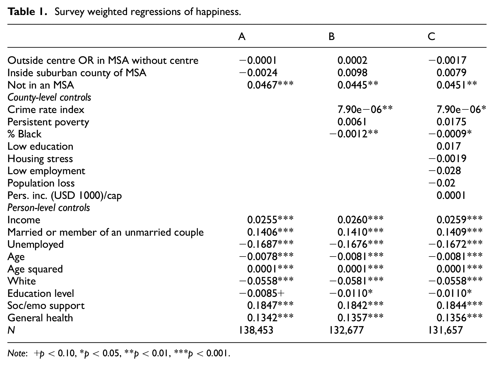
Note: +p < 0.10, *p < 0.05, **p < 0.01, ***p < 0.001.
We start with a person-level location variable. City size dummies are listed first in the table and indicate difference relative to the centre city. The most significant, both statistically and practically, is the ‘not in MSA’ dummy. As hypothesised, people are happiest outside of cities. Estimates are stable across specifications; it does not matter whether the city has stereotypical urban problems. People living outside of metropolitan areas as compared with central cities are happier by 0.05 on a scale from 1 to 4. This difference may appear to be small in practical terms, but it is still important. First, it contradicts claims that people are happier in cities, notably those by Glaeser (2011). Second, happiness is largely due to person-level influences such as unemployment, and ecology is secondary. Across 232 counties in our sample, happiness ranges between 3.18 and 3.56, with the vast majority of counties, 209 of the 232, in the 3.30 and 3.40 ranges. Third, an ecological difference of 0.05 (coefficient on ‘not in an MSA’ from Table 1) on a happiness scale from 1 to 4 can translate to large effects: for example, all else being equal, if one-third of 1% of the US population, about 1 million people, who live in central cities instead lived in non-urban areas, it would mean about 50,000 (0.05*1 million) people would be satisfied with their lives rather than dissatisfied.
All person-level variables are significant, while most county-level variables are not significant. It could be that the location variable is significant because of the large sample size at the person level. Yet, in Table 2 we use a county-level size variable, the urban–rural continuum. It ranges from 1 (‘metro>1 million’) to 9 (‘non-metro<2500, not adjacent to metro’). This triangulation of measurement serves as a robustness check; the smaller the place, the more happiness, no matter how the city is measured.
Survey weighted regressions of happiness.
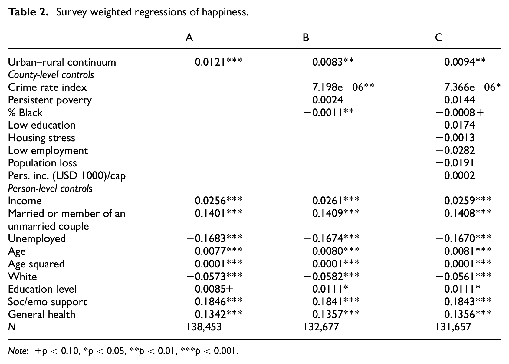
Note: +p < 0.10, *p < 0.05, **p < 0.01, ***p < 0.001.
The coefficient estimates are 0.01, and there are eight categories on the urban–rural continuum, so a change from 1 (‘metro>1 million’) to 9 (‘non-metro<2500, not adjacent to metro’) is associated with a happiness difference of about 0.1. What is striking about this second set of results is the persistence of statistical significance at the p < 0.01 level on the urban–rural continuum variable; the significance of all county-level control variables is much less stable. Urban unhappiness exists, and hence we find support for hypotheses H1a and H1b. To account for possible lag effects from contextual, county-level variables on happiness, we reran these models using the 2006, 2007 and 2008 BRFSS data (the results are in the appendix, available online).
Finally, Table 3 shows that the denser the county, the less happy people are there. Adding controls attenuates the effect. Crime and poverty explain away some of the city effect. Percent Black also explains some of the city effect. Yet, density remains negative and significant when controlling for a full set of covariates.
Survey weighted regressions of happiness.
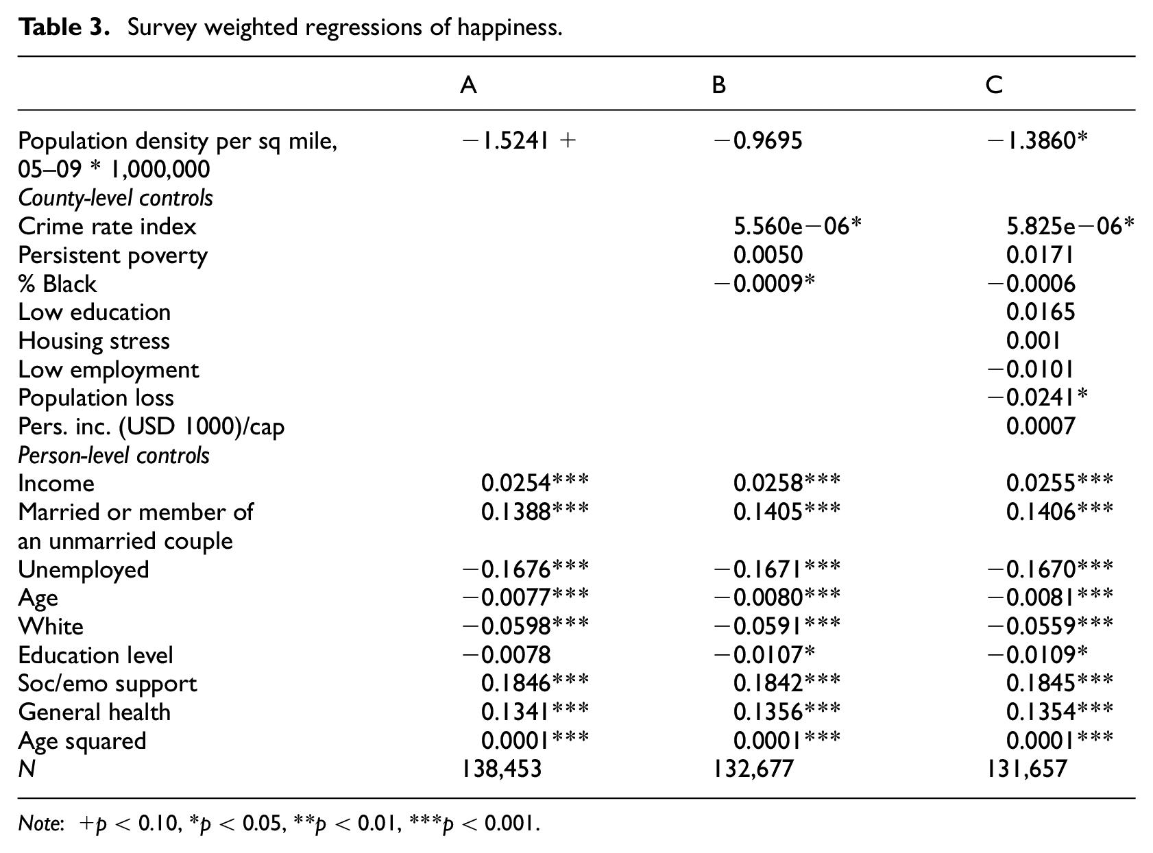
Note: +p < 0.10, *p < 0.05, **p < 0.01, ***p < 0.001.
Results from all models are consistent. Defining the city in multiple ways and controlling for commonly considered urban problems and other characteristics changes the results little, which suggests that it is the defining features of cities – size and density – that are responsible for the urban–rural happiness gradient, indicating support for hypothesis H2. Solving urban problems, if it were possible, would not likely make people in cities as happy as people are elsewhere. Urbanism – in terms of large population size and high density – is associated with lower happiness.
Fixed effects survey weighted regressions of happiness.

We use a county fixed effects model to account for potential omitted variable bias, any unobserved heterogeneity, and anything specific about the area that may affect results. US cities differ from each other substantially. It is not possible to control for all urban problems (or all confounding variables), but any such factors would be picked up in the fixed effects model. Lower happiness in urban areas persists in the fixed effects model.
Finally, we focus on several specific cases and make some illustrative comparisons. A ranking of happy counties (table 8 in the appendix, available online) shows that the happiest counties are not cities, and the least happy counties are large cities. The three happiest counties (happiness > 3.5) in this sample are rural, yet close to large cities. They therefore have the amenities nearby that cities offer, but they escape potential downfalls of larger size and higher density. Douglas County, CO, borders Denver, but remains largely rural and has a population density of 300/sq. mile. Shelby County, TN, is partially urban; it houses Memphis, yet most of the county is rural and the population density is relatively low at 1200/sq. mile. Johnson County, KS, is mostly rural, yet close to Kansas City and has a population density of 1100/sq. mile. On the other side of the scale, the counties with the lowest happiness scores (happiness < 3.2) in this sample are urban: the first one, St Louis city, MO, is all urban; it covers the central city of St Louis, and has about five times the population density of two of the three happiest counties, at 5700/sq. mile (and 19 times the density of the happiest county). The second and third least happy counties, Bronx, NY and Kings, NY (Brooklyn) are parts of the American city with the largest population, New York City; both counties have a density of over 30,000/sq. mile. The happiness differences between urban and non-urban counties, even though they appear small, are substantial because most people (>90%) are either satisfied ‘3’ or very satisfied ‘4’ with their lives and the standard deviation across counties in this sample is only 0.06. Hence, the urban–rural happiness gradient is quite substantial relative to the overall variability.
Discussion and future research
Fischer asked the right question about urban unhappiness: is it the city itself – in terms of its core characteristics of size and density – or is it what are typically thought of as urban problems that generate unhappiness? We have excluded alternative explanations (our controls and fixed effects at the county level), that urban problems such as poverty or crime are solely responsible for urban unhappiness. We have confirmed that people are less happy in cities, in part because of population size and density, the defining features of the city. Other variables also have an effect, but size and density matter, controlling for urban problems.
There is clearly a ‘city paradox’: cities provide sought-after resources, but we pay a price: the relative unhappiness of city life. High-density living fosters specialisation, information exchange, labour pooling, skills matching, knowledge spillovers, and more. On the other hand it can also foster crime, spread of disease, stress, cognitive and sensory overload, and other problems. Cities act like a magnifying glass, bringing out the best and the worst in us. This synergy has been estimated at the rate of 1.15 relative to the population – doubling population size increases everything (say crime or creativity) that an average person does by 15% (Bettencourt et al., 2007, 2010). Cities do not make people happier as Glaeser (2011) argues. People prefer to live outside of cities (Fuguitt and Brown, 1990; Fuguitt and Zuiches, 1975; Palmer, 2012) and, as we document here, people are happier outside of them.
Yet Americans are moving to metropolitan areas. This may point to an explanation of the Easterlin Paradox (1974) that economic growth does not result in happiness growth; perhaps this is due to people moving to less happy places. 9 Moving to a city will not necessarily make one less happy, nor will moving to a small town or village make one more happy. How moving to an area affects personal happiness is beyond the scope of this cross-sectional study. Yet, there is an urban–rural happiness gradient and it persists, regardless of urban problems such as poverty or crime. By pointing to urban unhappiness, we do not argue that urbanisation should be countered. There are many benefits to cities, and of course, some people are happier in cities than they would be elsewhere.
This study is about the USA and its results should not be generalised to other countries. At best these results can be generalised to other developed countries. However, in developing countries, there is likely to be a negative relationship between happiness and the city (Berry and Okulicz-Kozaryn, 2009).
As with any study, there needs to be more work done in this area; even though we continue a long-standing line of research, this is the first study to use county-level data to investigate the urban unhappiness hypothesis empirically. Future research may study how neighbourhoods (for example, census tracts) affect the wellbeing of residents. Cities are collections of neighbourhoods, and all characteristics, including happiness and urban problems, are distributed unevenly within a city and across its neighbourhoods. There are notable spatial inequalities (Ballas, 2013), so segregation and inequality are key fields for future work. Finer geographic resolution also has disadvantages; there are no surveys representative of neighbourhoods across a wide range of cities, so a neighbourhood study is not an alternative or an improvement over the present study but a complement to it. While neighbourhoods often seem independent or self-contained (‘a mosaic of little worlds which touch but do not interpenetrate’ (Park, 1915: 608)), there are spillovers as well; for example, poverty and crime in one neighbourhood does indirectly affect people and their happiness in other neighbourhoods. While people in public space may not engage in focused interaction, effectively being ‘alone, together’, people do encounter others in public transportation and in public spaces, especially in large cities (Morrill et al., 2005; Putnam, 2001).
Future research would do well to investigate why people choose to live in cities, given that urbanites are less happy, using person-level panel data. Future work might also explore the effect of the city on the happiness of different social groups. Additional research could use case studies of the happiest cities as opposed to the least happy cities and investigate more deeply than is possible with currently available data what makes residents happy. As more data become available, future research can focus on the exploration of multiple advantages and disadvantages of cities. We have striven to include the most important and easily measurable controls, but it is important to extend this research further by including an even larger set of city characteristics in the future. Notably, segregation, inequality, various types of pollution, and natural amenities are topics for future research in this area (Ballas, 2013; Brereton et al., 2008).
It may be possible that ‘deviant’ people choose to live in cities – and they may be less happy than are others and so that may depress overall city happiness. Indeed, Wirth (1938) argued that deviance would be higher in cities; Fischer (1995) referred to this as unconventionality, a more positive framing, but with the same notion that people with unusual interests or members of small subcultures would be more common in cities. These qualities may be to some degree picked up by person-level controls: income, education and unemployment, and by the county-level in the crime rate index. But otherwise, there is room for improvement, and future research could help in this area. In general, though, deviance and ‘qualities that make people unhappy’ are difficult to measure. There is also a possibility that unhappy people are pulled to cities; people who feel they do not belong in smaller areas and people who are unhappy where they live migrate to cities, but it is possible that even after urban migration their happiness remains. LGBTQ people (e.g. Doderer, 2011) and immigrants (e.g. Damm, 2009) prefer cities. But it is equally possible that happy and energetic extroverts move to cities to realise their full potential.
While there may be an element of self-selection, we think that it is possible that cities have the ability to change people in such a way that they become less happy. For instance, cities may intensify the pecuniary and consumerist orientation in people, and make them more stressed and overworked. Indeed:
To say that self-selection explains some of the differences between town and city is not to say that urbanism is irrelevant to those very same differences. It remains an indirect cause by stimulating selective migration. Although, part of urban/nonurban self-selection is coincidental, most of it results from processes originating in the nature of urbanism itself. (Fischer, 1982: 256)
And this is our interpretation and conclusion: urbanism is at least partially responsible for lower happiness in cities, regardless of urban problems.
Footnotes
Acknowledgements
We thank Michael Timberlake, the North American Editor of Urban Studies, whose comments on earlier writings by one of us (Okulicz-Kozaryn) on this subject inspired this study – to search for the effects of city size per se as opposed to the effects of compositional differences of bigger cities. We thank Paul Jargowsky and Arielle Kuperberg for their advice and comments, and our fellow affiliated scholars of the Center for Urban Research and Education at Rutgers-Camden for pushing us to be clearer in our argument. We are also grateful to the students in our courses, who have helped us think and rethink ideas about cities, but we take full responsibility for weaknesses in our arguments.
Funding
This research received no specific grant from any funding agency in the public, commercial, or not-for-profit sectors.