Trip and parking generation rates for different housing types: Effects of compact development

Abstract

Chinese

Guidelines for trip and parking generation in the United States come mainly from the Institute of Transportation Engineers (ITE). However, their trip and parking manuals focus on suburban locations with limited transit and pedestrian access. This study aims to determine how many fewer vehicle trips are generated and how much less parking demand is generated, by different housing types (single-family attached, single-family detached, and apartment and condo) and in different settings (from low density suburban environments to compact, mixed-use urban environments). Using household travel survey data from 30 diverse regions of the United States, we estimate a multilevel negative binomial model of vehicle trip generation and a multilevel Poisson model of vehicle ownership, vehicle trip generation and vehicle ownership being logically modelled as count variables. The models have the expected signs on their coefficients and have respectable explanatory power. Vehicle trip generation and vehicle ownership (and hence parking demand) decrease with the compactness of neighbourhood development, measured with a principal component that depends on activity density, land use diversity, percentage of four-way intersections, transit stop density and employment accessibility (after controlling for sociodemographic variables). The models capture the phenomena of ‘trip degeneration’ and ‘car shedding’ as development patterns become more compact. Reducing the number of required parking spaces, and vehicle trips for which mitigation is required, creates the potential for significant savings when developing urban projects. Guidelines are provided for using study results in transportation planning.

Keywords

car shedding compact development parking generation trip degeneration trip generation

Introduction

Vehicle use and ownership are of interest from the standpoints of energy, environment and transportation. Over half of the world’s oil and about 30% of total commercial world energy are consumed by the transport sector. In 2013, about 31% of total US CO₂ emissions and 26% of total US greenhouse gas emissions were generated by transportation (US EPA, 2015). Vehicle trip generation and vehicle ownership models are used by policy makers to identify factors that affect vehicle miles travelled (VMT), and therefore to address problems related to energy consumption, air pollution and traffic congestion (Dargay et al., 2007; Schipper, 2011).

Guidelines for trip and parking generation in the United States come mainly from the Institute of Transportation Engineers (ITE). The ITE Trip Generation Manual and Parking Generation manual are considered ‘bibles’ in transportation planning. However, these manuals focus on suburban locations with limited transit and pedestrian access. This study aims to determine how many fewer vehicle trips are generated, and how much less parking demand is generated, by different housing types in different settings, from low density suburban environments to compact, mixed-use urban environments.

It does so with the largest sample of travel and vehicle ownership data ever collected outside the National Household Travel Survey (NHTS) of 2009. The use of data for single regions, the specification of different models in each study and the use of different metrics to represent the built environment preclude the use of models for general transportation planning purposes. By contrast, this study pools data from 30 diverse regions of the US and uses consistently defined metrics to estimate best-fit vehicle trip generation and vehicle ownership models of three different types of housing (single-family attached, single-family detached, and apartment and condo).

Literature review

The built environment

In travel research, influences of the built environment on travel have often been named with words beginning with D – density, diversity, design, destination accessibility and distance to transit (Ewing and Cervero, 2010). While not part of the environment, demographics are the sixth D, controlled as confounding influences in travel studies.

Table 1 indicates how D variables are typically measured. Note that these are rough categories, divided by ambiguous and unsettled boundaries that may change in the future. Some dimensions overlap (e.g. diversity and destination accessibility). Still, it is a useful framework to organise the empirical literature and provide order-of-magnitude insights.

Table 1.

The D variables.

D variable	Measurement
Density	Density is always measured as the variable of interest per unit of area. The area can be gross or net, and the variable of interest can be population, dwelling units, employment or building floor area. Population and employment are sometimes summed to compute an overall activity density per areal unit.
Diversity	Diversity measures pertain to the number of different land uses in a given area and the degree to which they are balanced in land area, floor area or employment. Entropy measures of diversity, wherein low values indicate single-use environments and higher values more varied land uses, are widely used in travel studies. Jobs-to-housing or jobs-to-population ratios are less frequently used.
Design	Design measures include average block size, proportion of four-way intersections and number of intersections per square mile. Design is also occasionally measured as sidewalk coverage (share of block faces with sidewalks); average building setbacks; average street widths; or numbers of pedestrian crossings, street trees or other physical variables that differentiate pedestrian-orientated environments from auto-orientated ones.
Destination accessibility	Destination accessibility measures ease of access to trip attractions. It may be regional or local. In some studies, regional accessibility is simply distance to the central business district. In others, it is the number of jobs or other attractions reachable within a given travel time, which tends to be highest at central locations and lowest at peripheral ones. The gravity model of trip attraction measures destination accessibility. Local accessibility is a different animal, usually measured as distance from home to the closest shop.
Distance to transit	Distance to transit is usually measured as an average of the shortest street routes from the residences or workplaces to the nearest rail station or bus stop. Alternatively, it may be measured as transit route density, distance between transit stops or the number of stations per unit area. In this literature, frequency and quality of transit service are overlooked.

Source: Ewing and Cervero (2001, 2010); Ewing et al. (2015); Leck (2006); Saelens and Handy (2008); Stevens (2017).

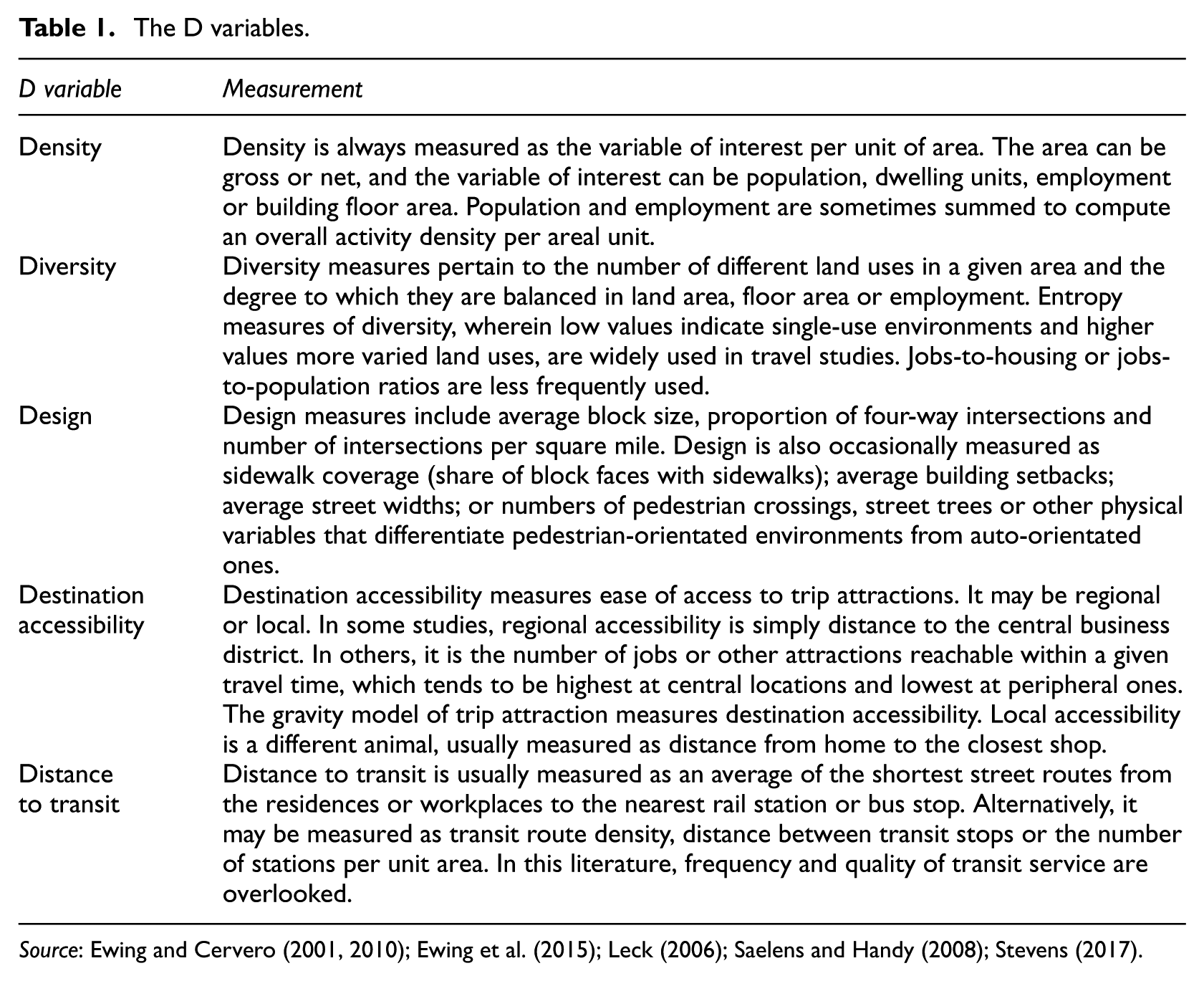
As the D values increase (except distance to transit, with an inverse relationship), the generalised cost of travel by alternative modes decreases, relative utility increases and mode shifts occur.

Vehicle trip generation and degeneration

The ITE Trip Generation Manual itself states that its ‘[d]ata were primarily collected at suburban locations having little or no transit service, nearby pedestrian amenities, or travel demand management (TDM) programs’ (ITE, 2012: 1). As a result, ITE methods overestimate vehicle trips generated at urban sites. A sample of 17 residential transit oriented developments (TODs) averaged 44% fewer daily vehicle trips than estimated by ITE (Arrington and Cervero, 2008). Another study found actual peak-hour trip rates to be between 26% and 50% lower than ITE rates for mid-rise apartments, general office buildings and quality restaurants at urban infill sites (Kimley-Horn and Associates, Inc., 2009). At 30 smart growth development sites in California, actual vehicle trip data showed 56–58% fewer vehicle trips than the ITE model predicted (Handy et al., 2013). In four out of five TOD cases, Ewing et al. (2017) found vehicle trip generation rates to be about half or less than half of what is predicted in the ITE Trip Generation Manual.

There are rich studies on the built environment and travel in the literature. A meta-analysis in 2010 found more than 200 individual studies of the built environment and travel (Ewing and Cervero, 2010). A more recent meta-regression analysis expanded this sample considerably (Stevens, 2017). The most common travel outcomes in these studies are VMT, walk trips and transit trips. Among the Ds, destination accessibility appears to have the strongest relationship to VMT, probably followed by street network design. The relationship of distance to transit to VMT is relatively weak, and the other two D variables have relationships that vary based on the specific method of calculation and the sample selected. The combined impact of these variables on VMT could be quite large (Ewing and Cervero, 2017).

A sixth D variable is demographics, which also affect household travel behaviour. The effects are not captured in the above meta-analysis or meta-regression, nor any literature review we are aware of. But individual studies would seem to indicate that demographics dominate the built environment when it comes to trip frequencies, that the built environment dominates demographics when it comes to trip lengths and that demographics have more effect on VMT than does the built environment – though both are important (Ewing and Cervero, 2001; Ewing et al., 2015).

Generalising across this vast literature, trip generation is a function of socioeconomic characteristics of travellers and the built environment. Compact developments that concentrate residents, workers and retail shops in close proximity to one another can ‘degenerate’ vehicle trips.

Vehicle ownership, car shedding and associated parking generation

Vehicle ownership and associated parking generation are one and the same. A household with two vehicles will generate peak demand for two parking spaces. The ITE Parking Generation manual notes that study sites upon which the manual is based are ‘primarily isolated, suburban sites’ (ITE, 2010). Studies show that vehicle ownership is lower in transit-served areas than in those that are not transit-served (Faghri and Venigalla, 2013; Zamir et al., 2014). By comparing parking-generation rates for housing projects near rail stops with parking supplies and with ITE’s parking-generation rates, Cervero et al. (2010) found there is an oversupply of parking near transit, sometimes by as much as 25–30 per cent. Oversupply of parking spaces may result in an increase in vehicle ownership, which is supported by the strong positive correlation between parking supply and vehicle ownership and auto use (Chatman, 2013; Guo, 2013; Weinberger, 2012).

There are many studies that have found additional relationships between vehicle ownership and built environmental variables. Households that live in dense, mixed-use and transit-served areas tend to own fewer automobiles, a phenomenon called car shedding; at the same time, they make more walking, bike and transit trips (Ewing and Tilbury, 2002). Studies have found that the built environment affects vehicle ownership, after controlling for the sociodemographic characteristics of households. All of the Ds have been related to vehicle ownership in one study or another (Cao et al., 2007; Chatman, 2013; Guo, 2013; Kim and Kim, 2004; Pinjari et al., 2011; Zegras, 2010). Ewing et al. (2017) found that peak parking demands in exemplary TODs, with all the Ds working for them, were less than half the numbers recommended by ITE in its Parking Generation manual.

Methodology

This study addresses the external validity issues with existing models by pooling household travel and built environment data from 30 diverse US regions and using a large number of consistently defined and measured built environmental variables to model vehicle ownership and use.

Household travel survey data

The most widely used data source to study travel behaviour is the household travel survey. Household travel survey data are the fundamental input for regional travel demand modelling and forecasting. Many Metropolitan Planning Organisations (MPOs) conduct their own travel surveys. We have contacted more than 100 MPOs with a population of at least 100,000 within their regions to obtain travel and supporting built environmental data. This has been a five-year effort.

We now have a convenience sample of data for 34 regions. Regions had to offer regional household travel surveys with XY coordinates, so we could geocode the precise locations of residences and capture the built environment for households more accurately than using predefined and aggregated geographic units. It is not easy to assemble databases that meet this criterion, as confidentiality concerns mean that MPOs are often unwilling to share XY travel data. In addition, for this study, household travel data had to be from the past decade. Travel behaviour has been changing as lifestyles change. We could have further limited our sample to newer surveys, but at the cost of degrees of freedom and generalisability. This constraint reduced our dataset to 30 regions across the United States. The regions are as diverse as Boston and Portland at one end of the urban form continuum and Houston and Atlanta at the other.

To compare the residential trip generation in household travel surveys with ITE trip generation rates, we limited the trips and households using the following criteria: we only included driver-based vehicle trips (trips made by passengers in a vehicle were not counted); we only included home-based vehicle trips (trips made between non-home locations were not counted); we only included households where every member of the household provided a travel diary (many households provided incomplete trip records); and we only included households where the last trip for each person was home-based (many respondents forgot to report the last trip of the day, the one that takes them home).

The resulting pooled data set consists of 619,773 trips by 63,077 households (Table 2). To our knowledge, this is the largest sample of household travel records ever assembled for such a study outside of the National Household Travel Survey (NHTS) of 2009. And, relative to NHTS, our database provides much larger samples for individual regions and permits the calculation of a wide array of built environmental variables based on the precise locations of households. NHTS provides geocodes (identifies households) only at the census tract level.

Table 2.

Household travel survey dataset included in this study from 30 regions of the US.

Regions	Survey date	Surveyed households	Surveyed trips
Albany, NY	2009	882	7809
Atlanta, GA	2011	6900	71,127
Boston, MA	2011	6119	70,299
Burlington, NC	2009	373	3135
Charleston, SC	2009	139	1225
Dallas, TX	2009	1962	18,951
Denver, CO	2010	4499	46,597
Eugene, OR	2011	1347	14,002
Greensboro, NC	2009	1192	10,489
Hampton Roads, VA	2009	1419	11,807
Houston, TX	2008	4201	50,450
Indianapolis, IN	2009	2997	30,840
Madison, WI	2009	84	853
Miami, FL	2009	753	6267
Minneapolis-St. Paul, MN-WI	2010	6800	50,647
Orlando, FL	2009	530	4681
Phoenix, AZ	2008	2674	24,063
Portland, OR	2011	3633	40,151
Provo-Orem, UT	2012	1025	15,042
Richmond, VA	2009	382	3403
Rochester, NY	2011	2024	13,178
Salem, OR	2010	1317	13,592
Salt Lake City, UT	2012	2451	28,748
San Antonio, TX	2007	1147	11,804
Seattle, WA	2014	4123	34,869
Springfield, MA	2011	643	6722
Syracuse, NY	2009	409	3673
Tampa, FL	2009	1499	12,140
West Palm Beach, FL	2009	635	5024
Winston-Salem, NC	2009	918	8185
Total	—	63,077	619,773

Built environmental data

The regions included in our household travel survey sample were, in addition, able to supply GIS data layers for streets and transit stops, population and employment for traffic analysis zones (TAZs) and travel times between zones by different modes for the same years as the household travel surveys.

The XY coordinates from the household travel survey were geocoded by using GIS to identify locations of households. Road network buffers were built around household locations. Road network buffers have been proven more appropriate to study travel choice than circular buffers or any predefined spatial units such as TAZs, census block groups, etc. (Oliver et al., 2007; Tian and Ewing, 2017).

Point, line and polygon layer listed above were joined with road network buffers of household locations by using spatial analysis to obtain raw data, such as the number of intersections within buffers. These were then used to compute refined built environmental measures such as intersection density, which is simply the number of intersections divided by land area within the buffer. All of the GIS operations and spatial analysis were done by using ArcGIS 10.4 software.

Variables

Using these datasets, the built environment around a household’s home address was measured for buffers of different widths (quarter of a mile, half a mile and one mile street network distances). Ultimately, a half a mile buffer was chosen to define the relevant built environment, as a compromise which takes advantage of our precise household geocodes and optimises the explanatory power of our vehicle trip and parking generation models. The idea here is that people living in walkable and bikeable neighbourhoods will have alternatives to driving, and therefore will make fewer vehicle trips and own fewer automobiles. Also, half a mile is considered a common limit on people’s willingness to walk to transit. In fact, according to the 2009 NHTS, the average walk trip length in the United States varies by trip purpose from 0.52 miles for shopping trips to 0.88 miles for work trips. The overall average is 0.70 miles, which implies a relevant environmental scale of half a mile to one mile. Also, according to the 2009 NHTS, the average walk access trip to transit is about 0.52 miles.¹ Again, the relevant built environment would be half a mile to a mile from the destination people would be prepared to walk to.

Household income was provided in interval form in the raw data. The midpoint of each interval was assigned to the respective household. It was also adjusted for inflation by the percentage increase of the Consumer Price Index (CPI) from the survey year to 2012. Likewise, average state petrol price for the year of the survey, from the Texas Transportation Institute’s Annual Urban Mobility database, was included as a predictor variable, after being adjusted for inflation. This variable varies by year and by state, sometimes fairly significantly, and reflects the operating cost of an automobile.

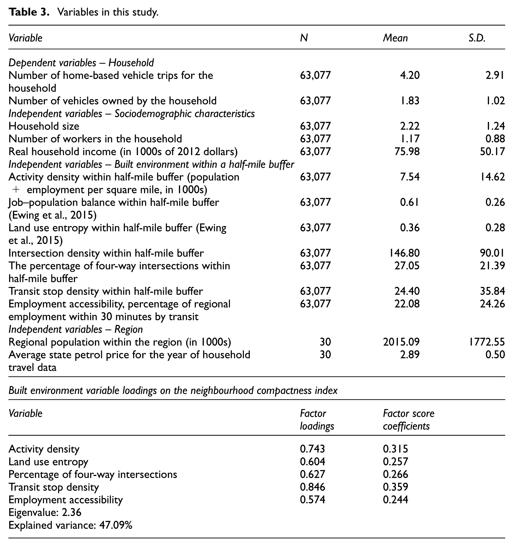
The dependent and independent variables used in this study are defined in Table 3. Sample sizes and descriptive statistics are also provided. The variables in this study cover all of the Ds, from density to demographics. With different measures, a total of 12 independent variables are available to explain household vehicle ownership and use. All variables are consistently defined from region to region. We categorised the types of house into three groups: single-family detached; single-family attached; and apartment and condo.

Table 3.

Variables in this study.

Variable	N	Mean	S.D.
Dependent variables – Household
Number of home-based vehicle trips for the household	63,077	4.20	2.91
Number of vehicles owned by the household	63,077	1.83	1.02
Independent variables – Sociodemographic characteristics
Household size	63,077	2.22	1.24
Number of workers in the household	63,077	1.17	0.88
Real household income (in 1000s of 2012 dollars)	63,077	75.98	50.17
Independent variables – Built environment within a half-mile buffer
Activity density within half-mile buffer (population + employment per square mile, in 1000s)	63,077	7.54	14.62
Job–population balance within half-mile buffer (Ewing et al., 2015)	63,077	0.61	0.26
Land use entropy within half-mile buffer (Ewing et al., 2015)	63,077	0.36	0.28
Intersection density within half-mile buffer	63,077	146.80	90.01
The percentage of four-way intersections within half-mile buffer	63,077	27.05	21.39
Transit stop density within half-mile buffer	63,077	24.40	35.84
Employment accessibility, percentage of regional employment within 30 minutes by transit	63,077	22.08	24.26
Independent variables – Region
Regional population within the region (in 1000s)	30	2015.09	1772.55
Average state petrol price for the year of household travel data	30	2.89	0.50
Built environment variable loadings on the neighbourhood compactness index
Variable	Factor loadings	Factor score coefficients
Activity density	0.743	0.315
Land use entropy	0.604	0.257
Percentage of four-way intersections	0.627	0.266
Transit stop density	0.846	0.359
Employment accessibility	0.574	0.244
Eigenvalue: 2.36
Explained variance: 47.09%

Principal component analysis

Rather than relying on multiple, correlated variables to represent the built environment around households, we chose to reduce many correlated variables to one factor, called a neighbourhood compactness index, representing the built environment around households. This factor was derived with principal component analysis (PCA), an analytical technique that takes a larger number of correlated variables and extracts a smaller number of factors that embody the common variance in the original data set.

Compactness indices have now been developed for metropolitan areas (Hamidi et al., 2015), census urbanised areas (Hamidi and Ewing, 2014) and metropolitan counties (Ewing et al., 2016b). In this article, we extend the practice to neighbourhoods, extracting (as in the earlier studies) a single variable from a set of five highly correlated D variables that captures nearly half of the variance in the original dataset.

At the smaller scale of the neighbourhood, other indices have been developed that mirror ours, such as Frank’s walkability index, which combines four D variables – net residential density, intersection density, land use mix and retail floor area ratio (FAR) – for each census block group, giving street connectivity twice the weight of the other three variables (Frank et al., 2005, 2006, 2010). Ours differs from Frank’s in that we consider all five types of D variables, use PCA to capture the common variance in the five and use buffers that are centred on the household location rather than on arbitrary census geography.

The principal component selected to represent the built environment was the first one extracted, the one capturing the largest share of common variance among the component variables and the one upon which the component variables loaded most heavily (Table 3). It is the only principal component with an eigenvalue greater than 1, a common cutoff point above which principal components are retained. All component variables load on this principal component with intuitively reasonable signs. Given the loadings, this principal component appears to represent the accessibility of residences to trip attractions outside the home.

As in earlier studies deriving compactness indices, we transformed the first principal component, which had a mean of 0 and standard deviation of 1, to a scale with a mean of 100 and standard deviation of 25, which we refer to as a neighbourhood compactness index. The range is from 67 to 577, meaning that the distribution is skewed to the right. There are a lot of neighbourhoods around the mean, but very few that are highly compact as we have measured compactness. Larger values correspond to greater compactness, as we have defined it and measured it with five variables via PCA.

To compute descriptive statistics and compare vehicle trip and parking generation rates with ITE, we have tried to rationalise the selection of cut points using standard deviations above and below the mean to define ranges. We define five levels of compactness, corresponding to more than one standard deviation below the mean (with index scores <= 75, 11.8% sample), between one standard deviation and the mean (with scores between 75 and 100, 46.4% sample), between the mean and one standard deviation above the mean (with scores between 100 and 125, 28.5% sample), between one standard deviation above the mean and two standard deviations above the mean (with scores between 125 and 150, 10.0% sample) and more than two standard deviations above the mean (with scores > 150, 3.4% sample). Vehicle trip rates and vehicle ownership rates follow smooth curves as we move from the most sprawling neighbourhoods to the most compact.

Multilevel modelling

To increase statistical power and external validity, we pooled data from 30 diverse regions. The data and model structure are hierarchical, with households ‘nested’ within regions. The best statistical approach for nested data is multilevel modelling (MLM), also called hierarchical modelling (HLM). MLM accounts for spatial dependence among observations (Raudenbush and Bryk, 2002). This dependence violates the independence assumption of ordinary least squares (OLS) regression and related statistical methods such as Poisson regression. Standard errors of regression coefficients based on these methods will consequently be underestimated. Moreover, coefficient estimates will be inefficient. Multilevel modelling overcomes these limitations, accounting for the dependence among observations and producing more accurate coefficient and standard error estimates (Ewing et al., 2015).

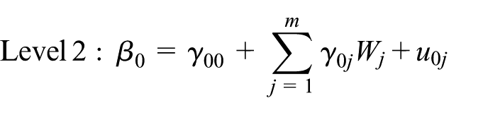
The multilevel models estimated in this study can be characterised as pairs of linked statistical models. At the first level (Level 1), household transportation outcomes are modelled within each region as a function of household characteristics plus a random error. Thus, each region has a region-specific regression equation that describes the association between household characteristics and outcomes. At the second level (Level 2), the region-specific intercept is conceived as outcomes, and is modelled in terms of regional characteristics plus random effects. Such models are often termed ‘random intercept’ models, to denote that only the intercept randomly varies (Raudenbush and Bryk, 2002).

Households living in a region such as Boston are likely to have very different vehicle trip generation or vehicle ownership characteristics compared with a region such as Houston, regardless of household and neighbourhood characteristics. The essence of MLM is to isolate the variance associated with each data level. MLM partitions variance between the household level (Level 1) and the regional level (Level 2) and then seeks to explain the variance at each level in terms of level-specific variables (Ewing et al., 2015).

The number of vehicle trips generated by a household and the number of vehicles owned by a household are count variables, which can only assume the values of zero, one, two or some larger positive integer. Two regression methods are used to model count variables – Poisson and negative binomial regression. They differ in their assumptions about the distribution of the dependent variable. Poisson regression is appropriate if the dependent variable is equi-dispersed, while negative binomial regression is appropriate if the dependent variable is overdispersed. Popular indicators of overdispersion are the Pearson and χ2 statistics divided by the degrees of freedom, so-called dispersion statistics. If these statistics are greater than 1.0, a model is said to be overdispersed (Hilbe, 2011: 88 and 142). By these measures, we have overdispersion of vehicle trips and near equi-dispersion of vehicle ownership rates, so the negative binomial model is appropriate for the former and the Poisson model is appropriate for the latter. Also, the frequency distributions of vehicle trips and vehicle ownership agree with the dispersion statistics (see examples in Figure 1 for the distributions of single-family detached housing). Models were estimated with HLM 7, Hierarchical Linear and Nonlinear Modelling software. Only the intercepts were allowed to vary randomly across level 2. All the regression coefficients at level 2 were treated as fixed and are called random intercept models (Raudenbush and Bryk, 2002). The two-level random intercept, multilevel Poisson and negative binomial regression equation is as follows:

Level 1 : E (Y | x_{1}, \dots x_{n}) = e^{β_{0} + \sum_{i = 1}^{n} β_{i} x_{i}}

Level 2 : β_{0} = γ_{00} + \sum_{j = 1}^{m} γ_{0 j} W_{j} + u_{0 j}

β_{i} = γ_{i 0}

Figure 1.

The distributions of vehicle trips and vehicle ownership for single-family detached housing.

Where: E refers to the estimated value of the dependent variable, β₀ refers to the intercept of the dependent variable at level 1, βi refers to the coefficients of independent variables at level 1, x_i refers to the independent variables at level 1, γ₀₀ refers to the overall intercept, γ_0j refers to the coefficients of independent variables at level 2, W_j refers to the independent variables at level 2, u_0j refers to the random error component for the deviation of the intercept and γ_i0 refers to the overall coefficients.

Results

Descriptive statistics

Vehicle trip generation and degeneration

Table 4 provides vehicle trip rates from our 30-region database, for three different housing types and five different levels of neighbourhood compactness. As expected, average trip rates per household are higher for single-family detached than single-family attached households, and for single-family attached than apartments and condos (multifamily units). Also as expected, average vehicle trip rates per household drop off with rising neighbourhood compactness.

Table 4.

Average vehicle trip generation rates by housing type from 30-region database, ITE Trip Generation Manual and NHTS.

30-region database
	Neighbourhoodcompactness index	Sample size	Vehicle trips (per household)	Vehicle trips (per person)
Single-family detached	< 75	6766	4.95	2.08
	75–100	23,952	5.04	2.17
	100–125	11,928	4.38	2.11
	125–150	3008	3.69	1.94
	> 150	240	2.87	1.47
	Average	45,894	4.76	2.12
Single-family attached	< 75	297	4.01	2.27
	75–100	2623	3.47	2.17
	100–125	2324	3.04	1.94
	125–150	921	2.57	1.50
	> 150	214	1.88	1.11
	Average	6379	3.17	1.96
Apartment and condo	< 75	200	3.27	2.03
	75–100	2053	3.10	2.01
	100–125	3172	2.57	1.74
	125–150	2072	1.82	1.32
	> 150	1502	1.21	.88
	Average	8999	2.31	1.57
ITE Trip Generation Manual (weekday)
			Vehicle trips (per household)	Vehicle trips (per person)
Single-family detached (210)			9.52	2.55
Condominium/townhouse (230)			5.81	2.49
Apartment (220)			6.65	3.31
2009 National Household Travel Survey (NHTS)
		Sample size	Vehicle trips (per household)	Vehicle trips (per person)
Single-family detached		64,855	4.45	2.23
Single-family attached		13,994	2.87	1.90
Apartment and condo		4089	3.27	1.97

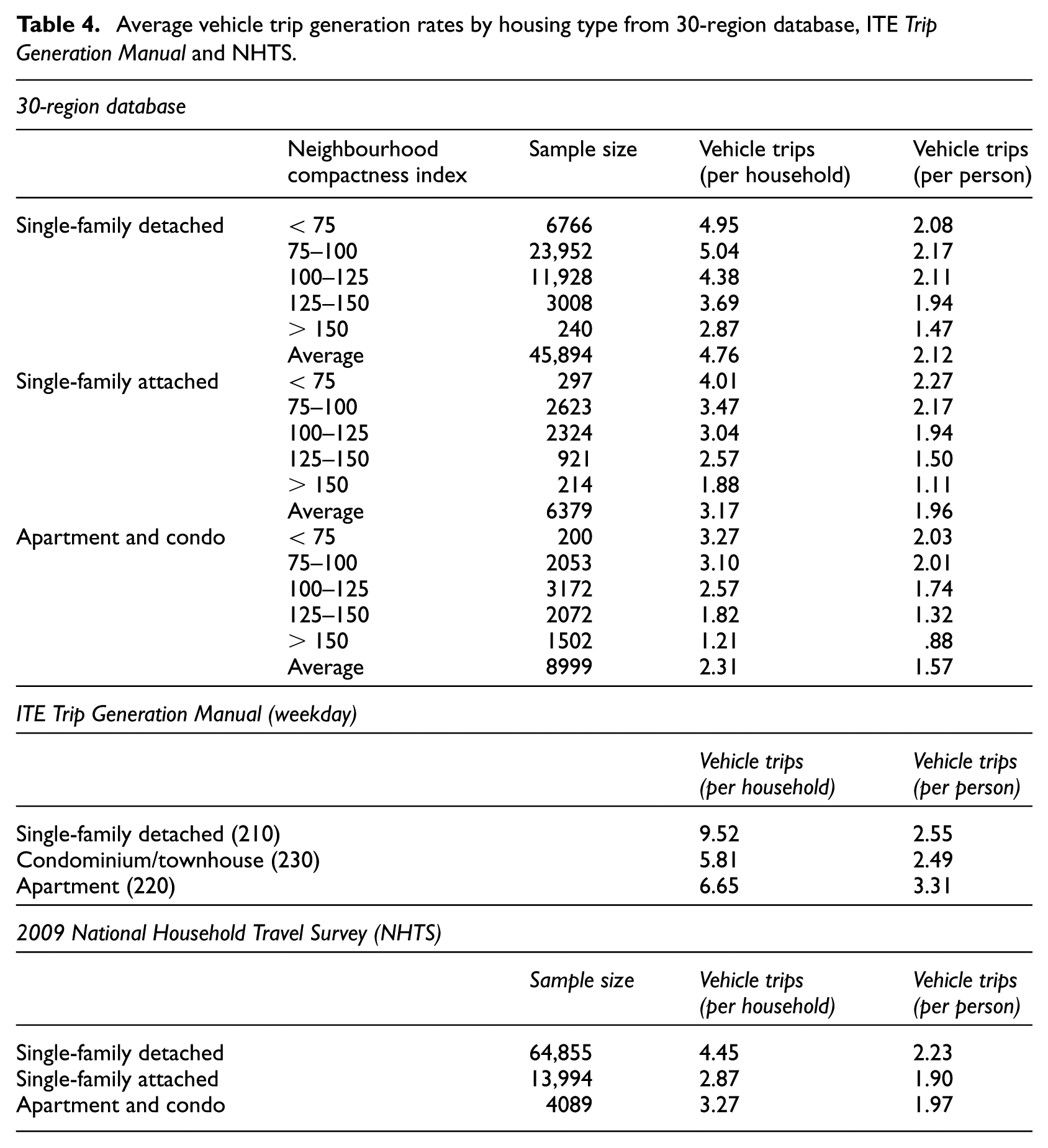
Two interesting patterns emerge. First, when vehicle trip rates are presented on a per person basis instead of a per household basis, differences among housing types and compactness levels partially disappear. That is to say, household size differences account for some (but not all) of the differences in vehicle trip rates. Second, the drop off in vehicle trip rates with compactness is far more pronounced between average and compact neighbourhoods than between sprawling and average neighbourhoods. Comparing the extremes, single-family households in sprawling neighbourhoods generate 2.08 vehicle trips per person per day, while multifamily households in compact neighbourhoods generate only 0.88 vehicle trips per person per day.

Table 4 also provides comparable (as nearly comparable as possible) vehicle trip generation rates from ITE and NHTS. Our rates are much lower than ITE’s, even with the bulleted data limitations indicated above. Again, part of the difference has to do with household size. The differences between ITE and self-reported rates are not as stark on a per person basis. But even on a person basis, our rates and NHTS rates are lower than ITE’s. This raises the question of why self-reported vehicle trip rates would be lower than automated driveway counts from individual housing developments. Self-reports could be biased downward, since people may forget about certain vehicle trips after the fact or may simply tire of inputting trip data. Also, our trip rates exclude package delivery trips to households in a development, visitor trips by friends and family, lawn and household maintenance trips, public service trips for rubbish collection and public safety and other trips that would not show up in a household travel diary survey.

The large disparity in trip generation rates on a per household basis suggests that any adjustments to ITE trip generation rates to account for the D variables should be applied only to the household’s own home-based trip rates, not to the difference between our rates and ITE’s.

Vehicle ownership and car shedding

Parking generation is more complicated than vehicle trip generation. There is both supply of and demand for parking. There is off-street and on-street parking, only the former of which is captured by ITE. And, of course, there are ITE guidelines and actual parking numbers for surveyed households.

Table 5 presents average vehicle ownership per household as a function of housing type and compactness level. As expected, households in single-family detached housing own more cars than those in single-family attached housing, and those in single-family attached housing own more than those in apartments and condos (multifamily housing). Also, as expected, households in sprawling neighbourhoods own more cars than those in average neighbourhoods, while those in average neighbourhoods own more cars than those in compact neighbourhoods.

Table 5.

Average vehicle ownership (and associated parking) by housing type from 30-region database, ITE Parking Generation and NHTS.

30-region database
	Neighbourhood compactness index	Sample size	Vehicle ownership (per household)	Vehicle ownership (per person)
Single-family detached	< 75	6766	2.33	1.04
	75–100	23,952	2.15	0.98
	100–125	11,928	1.87	0.95
	125–150	3008	1.63	0.89
	> 150	240	1.41	0.79
	Average	45,894	2.07	0.98
Single-family attached	< 75	297	1.78	1.01
	75–100	2623	1.44	0.92
	100–125	2324	1.24	0.80
	125–150	921	1.13	0.69
	> 150	214	1.03	0.60
	Average	6379	1.33	0.84
Apartment and condo	< 75	200	1.65	1.04
	75–100	2053	1.29	0.87
	100–125	3172	1.07	0.74
	125–150	2072	0.88	0.65
	> 150	1502	0.74	0.56
	Average	8999	1.03	0.73
ITE Parking Generation (weekday)
			Setting	Peak demand (vehicles per household)
Single-family detached (210)			—	1.83
Townhouse/condominium (230)			Suburban	1.38
Low/mid-rise apartment (221)			Suburban	1.23
			Urban	1.20
High-rise apartment (222):5 or more floors			Central city, not downtown	1.37
2009 National Household Travel Survey (NHTS)
		Sample size	Vehicle ownership (per household)	Vehicle ownership (per person)
Single-family detached		64,855	2.15	1.11
Single-family attached		13,994	1.25	0.84
Apartment and condo		4089	1.75	1.07

Again, two interesting patterns emerge. First, when vehicle ownership rates are presented on a per person basis instead of a per household basis, differences among housing types and compactness levels partially disappear. That is to say, household size differences account for some (but not all) of the differences in vehicle ownership rates. Second, the drop off in vehicle ownership rates with compactness is approximately the same between average and compact neighbourhoods as it is between sprawling and average neighbourhoods. Comparing the extremes, single-family households in sprawling neighbourhoods own 1.04 vehicles per person, while multifamily households in compact neighbourhoods own only 0.56 vehicles per person.

Table 5 also provides comparable (as nearly comparable as possible) vehicle ownership rates from ITE and NHTS. Our rates are lower than ITE’s. Again, part of the difference has to do with household size. The disparity in vehicle ownership rates on a per household basis suggests that adjustments to ITE vehicle ownership rates to account for the D variables are necessary.

Inferential statistics

Vehicle trip generation and degeneration

The best-fit multilevel negative binomial regression models for vehicle trip generation by different housing types are shown in Table 6. Also presented in Table 6 are measures of effect size, specifically elasticities of vehicle trips with respect to each of the independent variables. The elasticity in a negative binomial model is just the regression coefficient times the mean value of the independent variable.

Table 6.

Multilevel negative binomial regression for household vehicle trip generation.

Single-family detached household
	Coefficient	Standard Error	t-ratio	p-value	Elasticity
Intercept	1.104	0.076	14.553	< 0.001	—
Regional population	−0.00002	0.000008	−2.176	0.038	−0.040
Petrol price	—	—	—	—	—
Household size	0.170	0.011	15.150	< 0.001	0.413
Workers	0.122	0.007	16.369	< 0.001	0.156
Household income	0.002	0.0002	9.523	< 0.001	0.167
Neighbourhood compactness index	−0.002	0.0007	−3.183	0.002	−0.189
‘—’ This variable is not statistically significant at 0.05 level
Pseudo-R2: 0.32Highest VIF: 1.456
Single-family attached household
	Coefficient	Standard Error	t-ratio	p-value	Elasticity
Intercept	1.189	0.137	8.651	< 0.001	—
Regional population	−0.00003	0.000008	−3.391	0.002	−0.060
Petrol price	—	—	—	—	—
Household size	0.199	0.014	14.693	< 0.001	0.348
Workers	0.151	0.022	6.797	< 0.001	0.131
Household income	0.002	0.0003	9.129	< 0.001	0.118
Neighbourhood compactness index	−0.006	0.001	−4.452	< 0.001	−0.661
‘—’ This variable is not statistically significant at 0.05 level
Pseudo-R2: 0.26Highest VIF: 1.554
Apartment and condo household
	Coefficient	Standard Error	t-ratio	p-value	Elasticity
Intercept	1.207	0.067	18.133	< 0.001	—
Regional population	—	—	—	—	—
Petrol price	—	—	—	—	—
Household size	0.128	0.009	14.135	< 0.001	0.198
Workers	0.136	0.010	13.991	< 0.001	0.116
Household income	0.003	0.0002	13.987	< 0.001	0.143
Neighbourhood compactness index	−0.007	0.0007	−9.787	< 0.001	−0.854
‘—’ This variable is not statistically significant at 0.05 level
Pseudo-R2: 0.60Highest VIF: 1.388

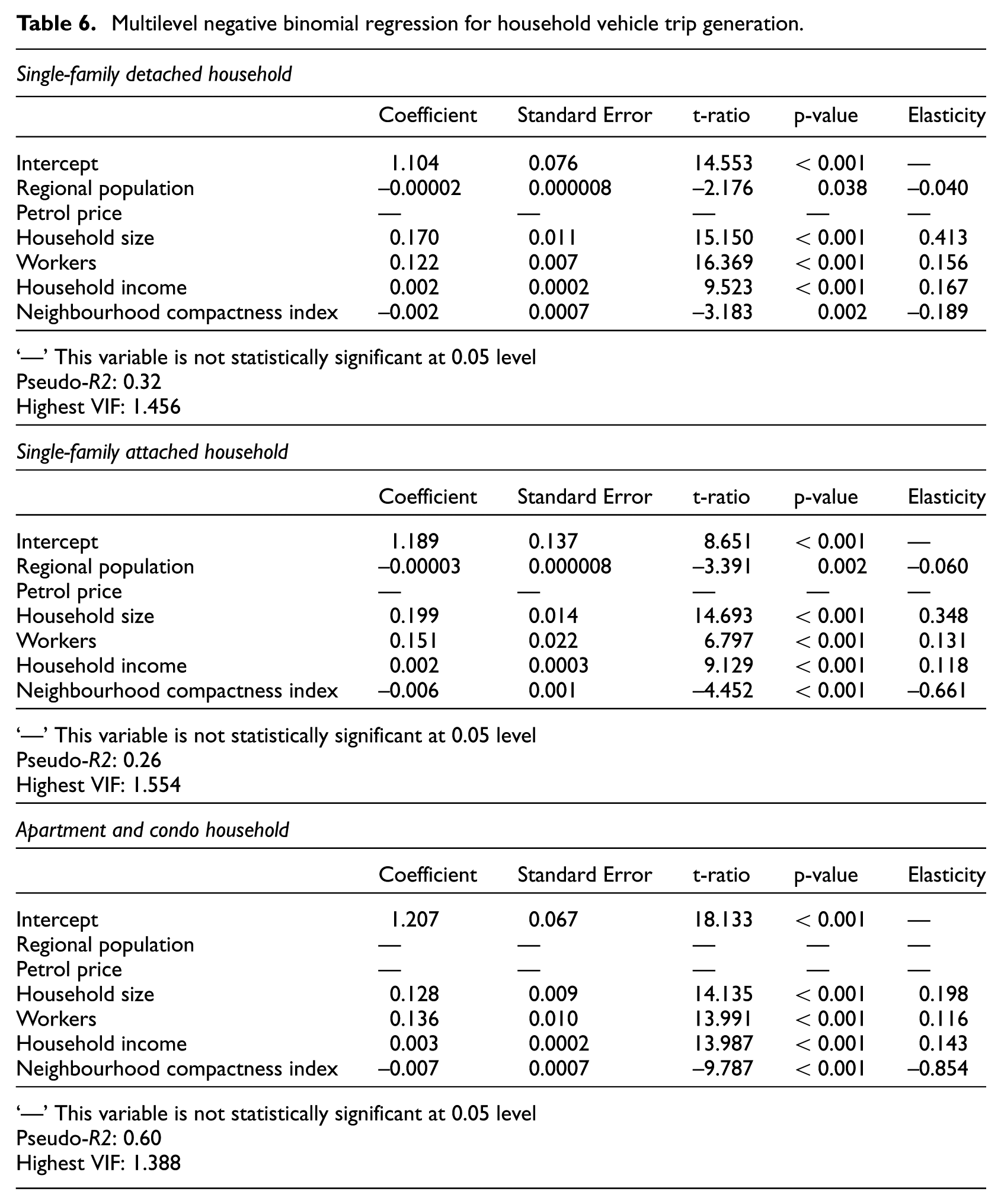
For all three types of housing, the number of vehicle trips generated by a household increases with household size, number of working members and household income. Bigger households with more workers and higher incomes tend to generate more vehicle trips.

We see evidence of trip degeneration as well. Controlling for socioeconomic variables, vehicle trip generation declines with neighbourhood compactness. This relationship suggests that areas with high population and employment densities, diverse land uses, good street connections, great transit service and high accessibility allow direct substitution of transit, walking and bike travel for automobile travel. This finding is in line with the literature generally (Ewing and Cervero, 2010; Ewing et al., 2015). The elasticities of vehicle trip frequency with respect to compactness, –0.661 for single-family attached housing and –0.854 for apartments and condos, are larger in absolute value than the elasticities of any other independent variables. It may also be the case that people in compact areas drive less due to the higher cost of driving, such as higher parking costs and lower driving speeds.

At the regional level, for single-family detached and attached housing, vehicle trips also decline with regional population. Larger regions typically offer much better transit service, which leads to substitution of transit trips for automobile trips.

The pseudo-R²s of the models range from 0.26 to 0.92. We have shown the pseudo-R² largely because urban planners are used to dealing with R²s and may want this information. Pseudo-R²s in multilevel regressions are not equivalent to R²s in OLS regression, and should not be interpreted the same way. The pseudo-R² bears some resemblance to the statistic used to test the hypothesis that all coefficients in the model are zero, but there is no construction of which it is a measure of how well the model predicts the outcome variable in the way that R² does in conventional regression analysis.

Vehicle ownership and car shedding

The best-fit multilevel Poisson regression models of vehicle ownership for different housing types are also shown in Table 7. Also presented in Table 7 are measures of effect size, specifically elasticities of vehicle ownership with respect to each of the independent variables. The elasticity in a Poisson regression model is just the regression coefficient times the mean value of the independent variable.

Table 7.

Multilevel Poisson regression for household vehicle ownership (and associated parking).

Single-family detached household
	Coefficient	Standard Error	t-ratio	p-value	Elasticity
Intercept	0.842	0.085	9.869	< 0.001	—
Regional population	—	—	—	—	—
Petrol price	−0.060	0.019	−3.124	0.005	−0.173
Household size	0.070	0.006	10.954	< 0.001	0.170
Workers	0.147	0.007	20.592	< 0.001	0.188
Household income	0.002	0.0002	10.082	< 0.001	0.167
Neighbourhood compactness index	−0.005	0.0004	−13.106	< 0.001	−0.473
‘—’ This variable is not statistically significant at 0.05 level
Pseudo-R2: 0.39Highest VIF: 1.459
Single-family attached household
	Coefficient	Standard Error	t-ratio	p-value	Elasticity
Intercept	0.393	0.126	3.108	0.005	—
Regional population	—	—	—	—	—
Petrol price	−0.056	0.025	−2.250	0.032	−0.162
Household size	0.123	0.018	6.670	< 0.001	0.215
Workers	0.190	0.027	7.187	< 0.001	0.165
Household income	0.003	0.0003	9.907	< 0.001	0.177
Neighbourhood compactness index	−0.005	0.0006	−9.321	< 0.001	−0.551
‘—’ This variable is not statistically significant at 0.05 level
Pseudo-R2: 0.92Highest VIF: 1.562
Apartment and condo household
	Coefficient	Standard Error	t-ratio	p-value	Elasticity
Intercept	0.555	0.286	1.944	0.062	—
Regional population	—	—	—	—	—
Petrol price	−0.147	0.083	−1.762	0.049	−0.425
Household size	0.128	0.009	14.545	< 0.001	0.198
Workers	0.211	0.019	11.375	< 0.001	0.179
Household income	0.004	0.0003	15.235	< 0.001	0.190
Neighbourhood compactness index	−0.005	0.0007	−7.657	< 0.001	−0.610
‘—’ This variable is not statistically significant at 0.05 level
Pseudo-R2: 0.61Highest VIF: 1.389

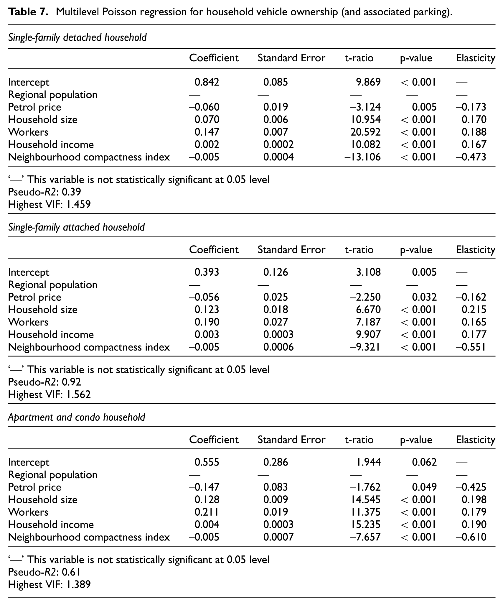
For all three types of housing, the number of vehicles owned by a household increases with household size, number of working members and household income.

We see evidence of car shedding as well. Controlling for socioeconomic variables, vehicle ownership declines with neighbourhood compactness. This relationship suggests that areas with high population and employment densities, diverse land uses, good street connections, great transit service and high accessibility allow direct substitution of transit, walking and bike travel for automobile travel, and thus car shedding. The elasticities of vehicle ownership with respect to compactness, –0.473 for single-family detached housing, –0.551 for single-family attached housing and –0.610 for apartments and condos, are larger in absolute value than the elasticities of any other independent variables. Note that, with one exception, these elasticities are smaller in absolute value than those of vehicle trip frequency. This seems plausible. Even those living in compact areas, who do not drive on a regular basis, may still desire the convenience of owning a car for leisure and other occasional activities.

At the regional level, for all three types of housing, vehicle ownership declines with petrol price. The elasticity of vehicle ownership with respect to petrol price for apartments and condos is larger than for single-family households. Multifamily households are more sensitive to petrol price than single-family households. Petrol price reflects the operating cost of an automobile. Although vehicle ownership is a fixed cost, higher operating costs discourage people from owning more vehicles. The pseudo-R²s of the models are 0.39 or higher. See the above discussion of pseudo-R²s in multilevel models.

Discussion and conclusion

Smart growth, as an alternative to auto-orientated sprawling development, encourages mixed residential and nonresidential land uses in walkable communities with transit options and nearby essential destinations. Increasingly, planners, scholars, innovative developers and local officials across the world promote smart growth as an antidote to many of the ills associated with urban sprawl. It is vitally important to accurately estimate the traffic impacts of a smart-growth development if communities are to reward such projects through lower exactions and development fees or expedited project approvals, and to right-size parking requirements. However, lacking a reliable methodology for adjusting trip and parking generation rates, communities relying on ITE guidelines are led to understate the traffic benefits of mixed-use development proposals and therefore discourage otherwise desirable developments.

This study explores how many fewer vehicle trips are generated and how much less parking demand is generated by different housing types in different settings, from low density suburban environments to compact, mixed-use urban environments. The results show that vehicle trip generation and vehicle ownership (and hence parking demand) decrease with the compactness of neighbourhoods after controlling for sociodemographic factors. In other words, the posited phenomena of ‘trip degeneration’ and ‘car shedding’ are borne out.

Applications to planning

How might the statistics in Tables 4 to 7 be used to plan for new developments? For the purpose of preliminary analysis or when the built environment and sociodemographic data are not available, a planner could estimate vehicle trip and parking generation from the descriptive statistics (Tables 4 and 5) showing average numbers aggregated from multiple regional household travel surveys. For three housing types – single-family detached, single-family attached and apartment and condo – and five levels of compactness in built environment setting, planners could apply the average vehicle trips and average vehicle ownership (per household or per person) to a specific development site.

On the other hand, with the complete data sets listed in Table 3, planners are able to predict more accurate and reliable values of vehicle trip and parking generation. The process of calculating these two values is laid out below.

First, planners need to collect all required built environment and sociodemographic data. Second, built environment variables must be converted to a compactness index for a neighbourhood (a half-mile buffer) around a given site.² Third, all values of independent variables must be entered into the regression equations in order to estimate vehicle trip generation or parking generation rates (Tables 6 and 7). Note that the predicted values in negative binomial and Poisson models are the logs of the expected values of the outcome variables. Thus, to derive estimates of vehicle trip generation and vehicle ownership, one needs to exponentiate the values from the regression equations, that is, take the anti-logs of the values.³

Additionally, in order to illuminate the region-specific intercepts that were estimated in the second level of the model, Figure 2 shows how the intercepts change with respect to regional population for vehicle trip generation and regional petrol price for vehicle ownership (and associated parking). This aspect of the models is a key feature of the specification and an important part of the rationale for using multilevel modelling. Planners can see how much variation exists between regions once socioeconomic variables and neighbourhood compactness have been controlled for. At the regional level, the intercept for vehicle trip generation decreases with the increase of regional population and the intercept for vehicle ownership decreases with the increase of regional average petrol price. The decreasing rates vary among different housing types.

Figure 2.

The region-specific intercepts.

Study limitations

We acknowledge a few limitations of this study. First, it may be difficult for local planners and engineers to collect and process the built environment data required for use of our tables. Some GIS data in the ‘Built environmental data’ section above might not be available at the local level or may require collaborations among multiple agencies. Also, data processing requires GIS skills such as network analysis. Most desirably, MPOs would collect, process and publish compactness metrics for subareas (traffic analysis zones perhaps) within their regions. We have done this for individual households in 30 regions, so it is doable.

Second, in Tables 6 and 7, we have presented elasticities with respect to the neighbourhood compactness index, a composite of five D variables. Results for the individual D variables are available upon request. We acknowledge that diverse impacts of built environment variables are glossed over by using a single measure of compactness to characterise the built environment. We acknowledge that the different D variables have different impacts on travel behaviour and vehicle ownership.

We thought seriously about presenting predictive equations for outcomes including several D variables, or presenting elasticities of outcome variables with respect to several D variables, from which outcomes could be computed starting with ITE rates. The reason for creating an index, rather than treating the D variables individually, is that we wanted to present vehicle trip rates and vehicle ownership (parking demand) in look-up tables that mimic ITE’s. Planners can conveniently consult 3 x 5 tables to predict trip generation and parking demand for a new development project. Parenthetically, we regressed our two outcome variables on the D variables individually, controlling for sociodemographics. All the D variables have the expected negative relationships to outcomes and are statistically significant.

Third, relying on conventional household travel surveys, this study did not control for attitudinal variables or residential self-selection effects. Only three of the regions included attitudinal variables in their surveys. Residential self-selection occurs if the choice of residence depends in a significant way on preferences for owning automobiles or choosing one mode of transportation over another (Cao et al., 2006; Ewing et al., 2016a). Such attitudes confound the relationship between the residential environment and travel choices or vehicle ownership. The benefits associated with compact urban development patterns – trip degeneration and car shedding in this study – may be overestimated or underestimated. The evidence is mixed (Ewing and Cervero, 2010; Ewing et al., 2016a; Stevens, 2017).

Fourth, while count regression models (negative binomial or Poisson regression) are commonly used in vehicle trip and parking generation studies, they treat car ownership as separate from vehicle trip generation when the two are actually linked (Anowar et al., 2014). Car ownership plays a mediating role in the complex relationship between the built environment and travel behaviour (Aditjandra et al., 2012). Using structural equation models, future research might be able to measure both the direct effect of the built environment on travel behaviour and the indirect effect via car ownership.

Fifth, household travel surveys may not be the most accurate source of vehicle trip generation estimates for residential developments. There are significant differences between our results and ITE trip generation rates due presumably to under-reporting of trips in household diary surveys plus delivery and visitor traffic not captured in household travel surveys. These create systematic downward bias that needs to be corrected in trip generation analysis.

Finally, this is a convenience sample of regions, not a random sample. There is an element of self-selection. But in our defence … we reached out to more than 100 regions in our effort to get every bit of travel data available. There is a certain randomness about which regions have conducted travel surveys recently, which have geo coded exact trip locations with XY coordinates and which are willing to release XY data to us. We have reduced the time spread of surveys to seven years, from 2007 on, so there is less bias associated with recency. The individual household travel surveys in the 30 regions are randomised, so it is only at Level 2 (the regional level) not Level 1 (the household level) that any bias would be present. And we modelled level 2 characteristics that might cause differences across regions. Consider how much less biased our 30-region sample is than the typical one-region sample that characterises most of the built environment-travel literature. Our results would not be expected to apply perfectly to any given region or subarea within a given region, particularly to small metropolitan areas and nonmetropolitan areas, since regions in our sample are large. As with the ITE vehicle trip and parking generation rates, planners and other users must be careful about extrapolating the results beyond the original sample.

Still, we believe that our results have the potential to improve ITE trip generation and parking generation estimates by explicitly accounting for trip degeneration and car shedding in compact, mixed-use urban environments (as compared with ITE’s sprawling, single-use suburban environments). They should not be viewed so much as a substitute for ITE rates but rather as a supplement to them that can be used by professional planners and engineers in project-specific trip and parking generation analyses.

Footnotes

Declaration of conflicting interests

The author(s) declared no potential conflicts of interest with respect to the research, authorship, and/or publication of this article.

Funding

The author(s) received no financial support for the research, authorship, and/or publication of this article.

ORCID iDs

Guang Tian

Keunhyun Park

Notes

References

Aditjandra

Cao

Mulley

(2012) Understanding neighbourhood design impact on travel behaviour: An application of structural equations model to a British metropolitan data. Transportation Research Part A: Policy and Practice 46(1): 22–32.

Anowar

Eluru

Miranda-Moreno

(2014) Alternative modeling approaches used for examining automobile ownership: A comprehensive review. Transport Reviews 34(4): 441–473.

Arrington

Cervero

(2008) TCRP report 128: Effects of TOD on housing, parking, and travel. Washington, DC: Transportation Research Board of the National Academies.

Cao

Handy

Mokhtarian

(2006) The influences of the built environment and residential self-selection on pedestrian behavior: Evidence from Austin, TX. Transportation 33(1): 1–20.

Cao

Mokhtarian

Handy

(2007) Cross-sectional and quasi-panel explorations of the connection between the built environment and auto ownership. Environment and Planning A 39(4): 830–847.

Cervero

Adkins

Sullivan

(2010) Are suburban TODs over-parked? Journal of Public Transportation 13(2): 47–70.

Chatman

(2013) Does TOD need the T? On the importance of factors other than rail access. Journal of the American Planning Association 79(1): 17–31.

Dargay

Gately

Sommer

(2007) Vehicle ownership and income growth, worldwide: 1960–2030. The Energy Journal 28(4): 143–170.

Ewing

Cervero

(2001) Travel and the built environment: A synthesis. Transportation Research Record: Journal of the Transportation Research Board 1780: 87–114.

10.

Ewing

Cervero

(2010) Travel and the built environment: A meta-analysis. Journal of the American Planning Association 76(3): 265–294.

11.

Ewing

Cervero

(2017) ‘Does compact development make people drive less?’: The answer is yes. Journal of the American Planning Association 83(1): 19–25.

12.

Ewing

Tilbury

(2002) Sketch Models for Integrated Transportation and Land Use Planning. Gainesville, FL: Gainesville Metropolitan Transportation Planning Organization.

13.

Ewing

Hamidi

Grace

(2016a) Compact development and VMT – Environmental determinism, self-selection, or some of both? Environment and Planning B: Planning and Design 43(4): 737–755.

14.

Ewing

Hamidi

Grace

(2016b) Urban sprawl as a risk factor in motor vehicle crashes. Urban Studies 53(2): 247–266.

15.

Ewing

Tian

Goates

et al . (2015) Varying influences of the built environment on household travel in 15 diverse regions of the United States. Urban Studies 52(13): 2330–2348.

16.

Ewing

Tian

Lyons

et al . (2017) Trip and parking generation at transit-oriented developments: Five US case studies. Landscape and Urban Planning 160: 69–78.

17.

Faghri

Venigalla

(2013) Measuring travel behavior and transit trip generation characteristics of transit-oriented developments. Transportation Research Board Annual Meeting 2397: 72–79.

18.

Frank

Sallis

Conway

et al . (2006) Many pathways from land use to health: Associations between neighborhood walkability and active transportation, body mass index, and air quality. Journal of the American Planning Association 72(1): 75–87.

19.

Frank

Sallis

Saelens

et al . (2010) The development of a walkability index: Application to the Neighborhood Quality of Life Study. British Journal of Sports Medicine 44(13): 924–933.

20.

Frank

Schmid

Sallis

et al . (2005) Linking objectively measured physical activity with objectively measured urban form: Findings from SMARTRAQ. American Journal of Preventive Medicine 28(2 Suppl. 2): 117–125.

21.

Guo

(2013) Residential street parking and car ownership: A study of households with off-street parking in the New York City region. Journal of the American Planning Association 79(1): 32–48.

22.

Hamidi

Ewing

(2014) A longitudinal study of changes in urban sprawl between 2000 and 2010 in the United States. Landscape and Urban Planning 128: 72–82.

23.

Hamidi

Ewing

Preuss

et al . (2015) Measuring sprawl and its impacts: An update. Journal of Planning Education and Research 35(1): 35–50.

24.

Handy

Shafizadeh

Schneider

(2013) California Smart-Growth Trip Generation Rates Study. Available at: http://downloads.ice.ucdavis.edu/ultrans/smartgrowthtripgen/Final_Report.pdf (accessed 24 February 2017).

25.

Hilbe

(2011) Negative Binomial Regression. 2nd edn. Cambridge, UK: Cambridge University Press.

26.

Institute of Transportation Engineers (ITE) (2010) Parking Generation. 3rd edn. Washington, DC: ITE.

27.

Institute of Transportation Engineers (ITE) (2012) Trip Generation Manual. 9th edn. Washington, DC: ITE.

28.

Kim

(2004) Effects of public transit on automobile ownership and use in households of the USA. Review of Urban and Regional Development Studies 16(3): 245–262.

29.

Kimley-Horn and Associates Inc. (2009) Trip-Generation Rates for Urban Infill Land Uses in California. Available at: http://www.dot.ca.gov/research/researchreports/reports/2009/final_summary_report-calif._infill_trip-generation_rates_study_july_2009.pdf (accessed 24 February 2017).

30.

Leck

(2006) The impact of urban form on travel behavior: A meta-analysis. Berkeley Planning Journal 19(1): 37–58.

31.

Oliver

Schuurman

Hall

(2007) Comparing circular and network buffers to examine the influence of land use on walking for leisure and errands. International Journal of Health Geographics 6(41): 1–41.

32.

Pinjari

Pendyala

Bhat

et al . (2011) Modeling the choice continuum: An integrated model of residential location, auto ownership, bicycle ownership, and commute tour mode choice decisions. Transportation 38: 933–958.

33.

Raudenbush

Bryk

(2002) Hierarchical Linear Models: Applications and Data Analysis Methods. 2nd edn. Thousand Oaks, CA: SAGE Publications, Inc.

34.

Saelens

Handy

(2008) Built environment correlates of walking: A review. Medicine and Science in Sports and Exercise 40(7 Suppl): S550–S566.

35.

Schipper

(2011) Automobile use, fuel economy and CO₂ emissions in industrialized countries: Encouraging trends through 2008? Transport Policy 18(2): 358–372.

36.

Stevens

(2017) Does compact development make people drive less? Journal of the American Planning Association 83(1): 7–18.

37.

Tian

Ewing

(2017) A walk trip generation model for Portland, OR. Transportation Research Part D: Transport and Environment 52: 340–353.

38.

United States Environmental Protection Agency (US EPA) (2015) Overview of Greenhouse Gases. Available at: https://www.epa.gov/ghgemissions/overview-greenhouse-gases#carbon-dioxide (accessed 24 February 2017).

39.

Weinberger

(2012) Death by a thousand curb-cuts: Evidence on the effect of minimum parking requirements on the choice to drive. Transport Policy 20: 93–102.

40.

Zamir

Nasri

Baghaei

et al . (2014) Effects of transit-oriented development on trip generation, distribution, and mode share in Washington, D. C., and Baltimore, Maryland. Transportation Research Record: Journal of the Transportation Research Board 2413: 45–53.

41.

Zegras

(2010) The built environment and motor vehicle ownership and use: Evidence from Santiago de Chile. Urban Studies 47(8): 1793–1817.