Does the monocentric model work in a polycentric urban system? An examination of German metropolitan regions

Abstract

Chinese

In explaining the determinants of urban spatial structure, researchers have relied on the traditional monocentric ‘Alonso-Mills-Muth’ model. This article contributes to this discussion by testing the viability of the monocentric model when applied to metropolitan areas in Germany, a country traditionally associated with a polycentric urban structure, regional differences and urban shrinkage. We estimate the model with a unique dataset covering 92 metropolitan areas over two time periods (2000 and 2014), which allows estimation in both a cross-sectional and a panel framework. Using spatial and panel regression techniques, we test whether the underlying determinants of urbanisation vary according to factors unique to the German context, including the roles of historical geography, regional polycentricism and urban shrinkage. We found that, similar to the US studies, the model performed reasonably well, particularly with the overall fit and the performance of the population variable, which was significant and positively related to urbanised area. Personal income and land prices showed mixed results, and the coefficients for transportation costs proved to be challenging. We also found that regional geography matters: a region in eastern Germany is smaller than one in the west. A proxy variable for regional polycentricity was not significant. Finally, we found that the model’s behaviour differs between growing and shrinking regions, most notably in the differing impacts that population change has on the change in urbanised area.

Keywords

agglomeration/urbanisation built environment economic processes land use monocentric model planning urban spatial structure

Introduction

The increasingly global and wide-ranging discussion on sprawl and urban growth patterns has produced attempts not only to empirically define, measure and quantify the phenomenon, but more importantly to better understand its drivers. Much of this work is based on North American metropolitan regions and datasets, but recent work has also addressed the operationalisation of urbanisation patterns in other regions, particularly Europe, China and Israel (Frenkel and Ashkenazi, 2008; Gao et al., 2016; Oueslati et al., 2015; Siedentop and Fina, 2010, 2012).

In explaining urban spatial structure, urban economists have relied on the traditional monocentric ‘Alonso-Mills-Muth’ model due to its simplicity and reliability (Brueckner and Fansler, 1983; McGrath, 2005; Oueslati et al., 2015; Paulsen, 2012, 2014; Spivey, 2008; Wassmer, 2006). These studies either examine a single city at a particular point in time or test the model with a cross-sectional sample of (usually) US cities. Several studies utilise a panel framework to estimate the impact of the independent variables on urbanised land area or the distance to the urban fringe (McGrath, 2005; Paulsen, 2012), including a rare study of European metropolitan areas (Oueslati et al., 2015). More recent studies apply sophisticated spatial regression analyses and expand the model to make it more suitable for polycentric metropolitan regions (e.g. Gómez-Antonio et al., 2016). Many of these studies have confirmed that the assumptions of the model – namely that urban area is a function of population, income, land values and marginal transportation costs – have held up under a wide variety of model specifications.

This article contributes to this discussion by testing the viability of the monocentric model when applied to metropolitan areas in Germany. In doing so, we assume that there are sufficient unique characteristics of German metropolitan urbanisation, including the role of historical geography, regional polycentricity, land market regulation and systemic urban shrinkage, to warrant different specifications and outcomes of the monocentric model. We expect that the spatial extent of German metropolitan regions will respond differently to the model compared with US regions. Specifically, German regions will be less responsive to changes in income and transportation, and to market forces more generally, due to the larger role of spatial planning and land use policy in determining urban form in Germany (Siedentop et al., 2016). Moreover, we expect the monocentric model to not perform as well in Germany, which has historically had a very polynucleated and polycentric settlement pattern. As such, we expect a lower goodness of fit, similar to Oueslati et al. (2015), who found a much lower goodness of fit for their study of European metropolitan areas. Furthermore, an empirical examination of German metropolitan areas allows us to test a number of hypotheses. These include the effectiveness of the model in explaining metropolitan areas given the role of the historical geography of eastern and western Germany 20 years after reunification, and the effectiveness of the model in explaining spatial structure in shrinking regions and in highly polycentric regions.

In specifying the monocentric model for Germany, we are able to utilise a consistent and continuous dataset and to test the variation in the robustness of the model across a number of dependent variables. We estimate a spatial regression model with a unique dataset covering 92 metropolitan areas over two time periods (2000 and 2014), which allows estimation in a cross-sectional model as well as a panel framework. We can therefore analyse if the model’s validity, as well as the dependent variables’, influence change over time.

Despite the focus on German metropolitan areas, this article is of interest to a broader international audience for a number of reasons. First, we contribute to the international comparative literature on the drivers of land use change, and expand the geographic scope of the monocentric model by empirically validating it using a unique dataset from Germany described above. Second, we contribute to the methodological development of the model by addressing issues of spatial autocorrelation through the specification of a spatial error model. Finally, we test a number of empirical hypotheses which will be of relevance to those interested in the drivers of urban spatial structure more broadly, in particular the role of polycentricity and urban shrinkage in determining urban spatial form. The rest of the article is organised as follows. First, we briefly review the theory and empirical research behind the monocentric model. Then we examine the literature particularly as it pertains to the construction and operationalisation of our variables. Next, we present cross-section estimates from a spatial error model and estimates from a fixed effects panel model on the determinants of urbanised land area. We also calculate the respective elasticities for the dependent variables for both cross-sectional and panel models, and disaggregate our dataset to understand whether the determinants of urban spatial structure differ for growing and non-growing metropolitan areas. Finally, we draw some conclusions and compare our models with each other as well as with similar studies.

The monocentric model

The monocentric model, commonly referred to as the Alonso-Mills-Muth model (henceforth AMM) after its initial developers (Alonso, 1964; Mills, 1972; Muth, 1969), was developed to explain urban land use and its relationship to urban land values. The AMM model is predicated on households maximising utility and having perfect knowledge of the market. Furthermore, all employment in the city takes place within a single Central Business District (CBD) and no housing durability or inertia exists in the housing market.

The AMM model requires five variables for an empirical estimation (Brueckner, 1987; Wheaton, 1974). The dependent variable assumes a concentric city with a radius of $x$ , and an urbanised land area of A ( $A = x^{2} π$ ) where $x$ is the city’s radius. The independent variables are urban population size (L), income (y), agricultural land rents (r_a) and transportation costs measured as per-mile monetary commuting costs as a function of distance to the urban centre ( $t = t (x)$ ).

For an equilibrium to hold, urban rents must equal agricultural rents at the urban fringe ( $r = r_{a} |_{x = \bar{x}})$ but outbid them inside the city ( $r > r_{a} |_{x < \bar{x}})$ , and population must fit into the urban area defined by the urban fringe $\bar{x}$ . Following the AMM model’s comparative static analysis provided by Brueckner (1987: 831–836), the independent variables’ effects on city size are as follows: $\frac{\partial A}{\partial L} > 0; \frac{\partial A}{\partial r_{a}} < 0; \frac{\partial A}{\partial y} > 0; \frac{\partial A}{\partial t} < 0$ .

Brueckner’s (1987: 831–836) economic intuition behind these effects gives the following results. An increase in population produces an increase in urbanised area $(\frac{\partial A}{\partial L} > 0)$ . Increasing demand for housing drives up prices since the existing urban area ( $\bar{x}$ ) cannot accommodate the higher population, which requires an expansion of urban area to ensure that $r = r_{a}$ at the urban fringe. Conversely, an increase in agricultural rents leads to a decrease in urban area $(\frac{\partial A}{\partial r_{a}} < 0)$ as it becomes more costly to develop land on the urban fringe. An increase in income causes the urban area to expand $(\frac{\partial A}{\partial y} > 0)$ as housing consumption increases, particularly along the urban fringe where land and housing is cheaper. Increasing incomes therefore cause the urban fringe to expand outwards to re-establish $r = r_{a}$ . An increase in transportation costs decreases the urban area $(\frac{\partial A}{\partial t} < 0)$ , as travelling any given distance becomes more expensive and central locations become more attractive.

Despite criticisms of the model for being overly static and not taking into account the increasingly fragmented and polycentric nature of many metropolitan growth patterns, previous empirical analyses find that the model holds up for the most part. Paulsen (2012: 562) provides an informative summary of a number of empirical studies, including Brueckner and Fansler (1983), Wassmer (2006) and Spivey (2008), all of which find that the model can explain a large portion of the variation in urban size (R²≥ 0.80) and where the independent variables (population, income and land price) have the expected sign. Measuring transportation costs adequately has proven to be challenging and has often resulted in unexpected signs. Oueslati et al. (2015) find that the AMM model only explains about a third of the variation in the amount of urbanised area in several European countries. This result is not unexpected, given the greater role that market forces play in determining urban spatial patterns in the US compared with European metropolitan areas. Finally, a comprehensive overview of empirical articles testing the AMM model and using the traditional urban spatial size as the dependent variable is provided by DeSalvo and Su (2019: 94). Interestingly, the authors find that most estimations are conducted using OLS specifications, thus neglecting spatial dependence.

Empirical basis: Geography, data and models

For our study, we utilise urban labour market regions (Städtische Arbeitsmarktregionen) from the German Federal Institute for Research on Building, Urban Affairs and Spatial Development (BBSR) as the unit of analysis. In this case, an urban labour market region is defined as adjacent counties (Landkreis) with at least 50 per cent of the population in large and medium sized cities of more than 25,000 inhabitants and a population density of at least 150 inhabitants per square kilometre, as well as counties outside of large and medium sized cities but with a population density of more than 150 inhabitants per square kilometre. Moreover, urban labour market regions are considered as functionally integrated areas based on commutes as a proxy for patterns of economic interconnection.

For the dependent variable, we utilise the amount of urbanised area (as defined by the Federal Office of Statistics) in 2000 and 2014. The urbanised area includes built-up land (residential, commercial, public use) as well as traffic areas and recreational areas such as public parks and sports facilities. These years were chosen because consistent data on land use (size of urbanised area) and independent variables at the level of counties (as the building blocks of urban labour market regions) were available.

US-based studies have tended to rely on Census of Agriculture data that include the median agricultural land value per acre at the county scale. Using these data, both Spivey (2008) and Paulsen (2012) calculate weighted average land values for each urbanised area in US dollars per acre, weighting by a county’s share of the metropolitan land area. To obtain a similar measure, we utilise average land price for potentially developable land (€/m²) from the Federal Office of Statistics. We feel this is a better approximation for the German context as only land designated as developable in a preparatory land-use plan (Flächennutzungsplan), which identifies future land uses according to projected needs, can be granted a building permit. The same office provides per capita income data that we use as well. For the panel estimation, monetary values were adjusted to 2010 values to ensure intertemporal comparability, using a price index which is published by the Federal Office of Statistics.

All US-based studies have difficulty operationalising transportation costs, as there is no direct monetary measure of commuting cost per mile, and in fact, neither Wassmer (2006) nor Paulsen (2012) include this variable in their model. As no Europe-wide data on transport costs exist, Oueslati et al. (2015) rely on highway density data from the Eurostat regional dataset as a proxy for transport costs, on the assumption that highway investment reduces the time and the costs of commuting. We utilise two different indicators – commuting time as a proxy for the opportunity cost of transportation, and average diesel prices per litre as a monetary cost measure. We utilise two separate variables, as we readily note that commuting time is not completely exogenous to the dependent variable (city size) and fuel prices better reflect the cost of transportation.

Commuting time is based on data from the German Federal Employment Agency, which provides origin–destination matrices for commuters travelling between their place of residence and their place of work by means of private automobile (and excludes public transportation trips). The Landkreise are assigned to urban labour market regions based on centroids, and the commuter number for each urban labour market region is computed by aggregating the data for Landkreise. Open street map data are used to create the network dataset required for network analysis. Travel times along the street network are computed for each origin–destination link, represented by centroids. Travel times for each labour market area are derived by aggregating the travel times calculated for each origin–destination link for two time periods (2002 and 2013). Although these dates deviate from our other variables (2000 and 2014), we argue that the commuting times are unlikely to have changed much between 2000 and 2002 or between 2013 and 2014. In some cases where residence and workplace are non-adjacent and in different states, the data were only available for administrative regions (NUTS2, so-called Regierungsbezirke). We assume that longer commutes should be correlated with both monetary and opportunity costs (see e.g. Glaeser and Kahn, 2004: 2493) and reflect the true cost of commuting. We also include an additional commuting variable which is similar in operationalisation but is much finer grained and utilises Verbandsgemeinden (municipality associations) instead of Landkreise. We feel this is a more robust proxy for commuting costs compared with Landkreise. Unfortunately, we only had these data for the year 2017, so they were only included in the model for the later time period, again implicitly assuming that travel times have not substantially changed between 2014 and 2017. However, for the panel model, we utilised only the Landkreis-based commuting variable, which has a lower resolution, due to the lack of available Verbandsgemeinde in the earlier time period.

For monetary cost, we utilise the yearly average cost of diesel for the region based on data collected by the Leibniz Institute for Economic Research. The Institute has collected data on fuel prices since Germany required all fuel stations to publish their prices beginning in 2013. The stations are geo-referenced and can therefore be linked to the labour market regions. While this variable more adequately captures the theoretical basis of the model, it is unfortunately only available for the later time period (2014).

In addition to these standard indicators, we also included two variables more specific to the general conditions in Germany. First, we hypothesise that regional variations exist in the ability of the model to explain urban spatial structure, particularly between eastern and western Germany. Since reunification, different economic, political and demographic conditions between eastern and western Germany have had differential impact on urban form and urban spatial structure (Schmidt, 2011). In order to control for this, we include a geographic dummy variable that takes a value of one if the region under consideration is located in former East Germany. Previous research (Schmidt et al., 2018) found that the East/West dummy was consistently significant and negative in explaining urban patterns. However, the unique conditions affecting urban spatial structure following the fall of the Berlin wall (for example specific economic incentives and subsidies) disappeared over time (Nuissl and Rink, 2003; Schmidt, 2011; Stanilov, 2007), suggesting declining differences between eastern and western urbanisation patterns. We therefore expect the model fit to change with time, too.

Second, Germany has a long tradition of decentralised and polycentric urban spatial development, and the degree of polycentricity of a metropolitan area will impact the ability of the model to explain the urbanised area size. The problem with applying the AMM model to a polycentric urban region is that the radian of the first city intersects with the radian of the second city at an urban rent level that is higher than agricultural rent $(r_{city 1} = r_{city 2} > r_{a} |_{x_{{1, 2}} < {\bar{x}}_{{1, 2}}})$ . Thus, these two (or more) cities merge into each other and create one bi- (or multi-)polar city. The AMM model has been modified with some limitations to explain such scenarios (e.g. see Fujita and Ogawa, 1982, for a linear city with two centres).

Spivey (2008) attempts to proxy the role of polycentric urban spatial structure on the model. She uses data from McMillen and Smith (2003), who estimated the number of sub-centres in over 60 large urban areas using commuting costs from the Texas Transport Institute. She finds that the coefﬁcient is negative (i.e. more sub-centres are associated with a smaller land area), and statistically signiﬁcant only at the 10 per cent level. Spivey concludes that sub-centres are more likely to develop in densely populated areas, or that increased density associated with sub-centre development helps to mitigate sprawl.

To control for polycentricity, we utilise information from the German central place system. According to their importance or rank in the urban hierarchy, these ‘central places’ provide services and infrastructure for the surrounding regions. Our proxy for polycentricity indicates the number of medium- and upper-level central places per capita in a labour market region. The greater the number of central places in a region, the greater is the degree of polycentricity. Using the number of central places has the added benefit of controlling for one of the primary state spatial planning and regional planning tools in Germany. The central place system regulates the growth opportunities of municipalities according to their central place status. Higher-tier central places usually have greater allowances for new development on previously non-developed land than lower-tier central places. Thus, we would expect the number of central places to be positively associated with urbanisation patterns.¹

Finally, we examine the model’s ability to explain the urban structure of shrinking cities. Urban decline is widespread in many regions experiencing deindustrialisation, particularly Eastern Europe, as cities and regions face post-socialist economic and political restructuring against a backdrop of longstanding demographic decline, an issue particularly acute in Germany (Müller and Siedentop, 2004; Nuissl and Rink, 2003). According to the model, population shrinkage should cause a decrease in the urbanised area. However, in reality we hardly ever observe a decrease in the urbanised area if population and/or income decreases (our dataset does not have any incidences where this occurs). Rather, municipalities may try to mitigate shrinkage by permitting additional greenfield development on the city’s periphery to attract new residents and firms, contrary to the model prediction. Because of this, we expect the empirical estimation of the AMM model to yield rather weak results for shrinking regions.

We also hypothesize that the overall explanatory ability of the model will be less than for the US counterparts due to the stronger role of government regulation in determining urbanisation patterns. This hypothesis is also consistent with Oueslati et al. (2015), who find that the model only explains about a third of the variation in the amount of urbanised area. However, as we control for a number of additional variables, we should nevertheless be able to identify the model’s overall relevance for the German context.

Descriptive statistics of all variables used in this study are found in Table 1. From an original dataset of 115 labour market regions, we omitted all regions with missing relevant variables (21) and then removed those regions without any neighbour according to first order Queen contiguity (2), reducing our sample size to 92 labour market regions.

Table 1.

Descriptive statistics of the variables used in this study.

Variable	Obs	Mean	Std. Dev.	Min.	Max.
Urbanised land area (in hectares)
2000	92	21,657.89	15,748.29	3612	100,420
2014	92	23,676.40	17,375.24	4368	111,134
Population
2000	92	508,876.1	508,090.0	77,106	2,707,494
2014	92	513,862.7	536,705.9	79,387	2,813,754
Per capita income (in €)^a
2000	92	16,359.28	1604.671	12,899.5	21,283.0
2014	92	21,739.77	2222.217	17,551.0	32,373.5
Average price of land (in € per m²)^a
2000	92	125.925	74.713	32.13	360.75
2014	92	158.808	119.764	43.43	941.07
Average commuting time (in minutes)
2002 (Landkreis-based)	92	17.373	2.465	11.6	24.8
2013 (Landkreis-based)	92	17.652	2.495	12.0	24.8
2017 (Verbandsgemeinde-based)	92	24.968	7.453	7.358	36.806
Diesel prices (in €)^a
2014	92	1.337	0.012	1.314	1.363
Central places per 100,000 inhabitants
2000	92	1.394	0.646	0.26	3.32
2014	92	1.408	0.657	0.27	3.24
Share of employees working in the core city/cities
2017	92	44.940	18.315	7.171	85.566

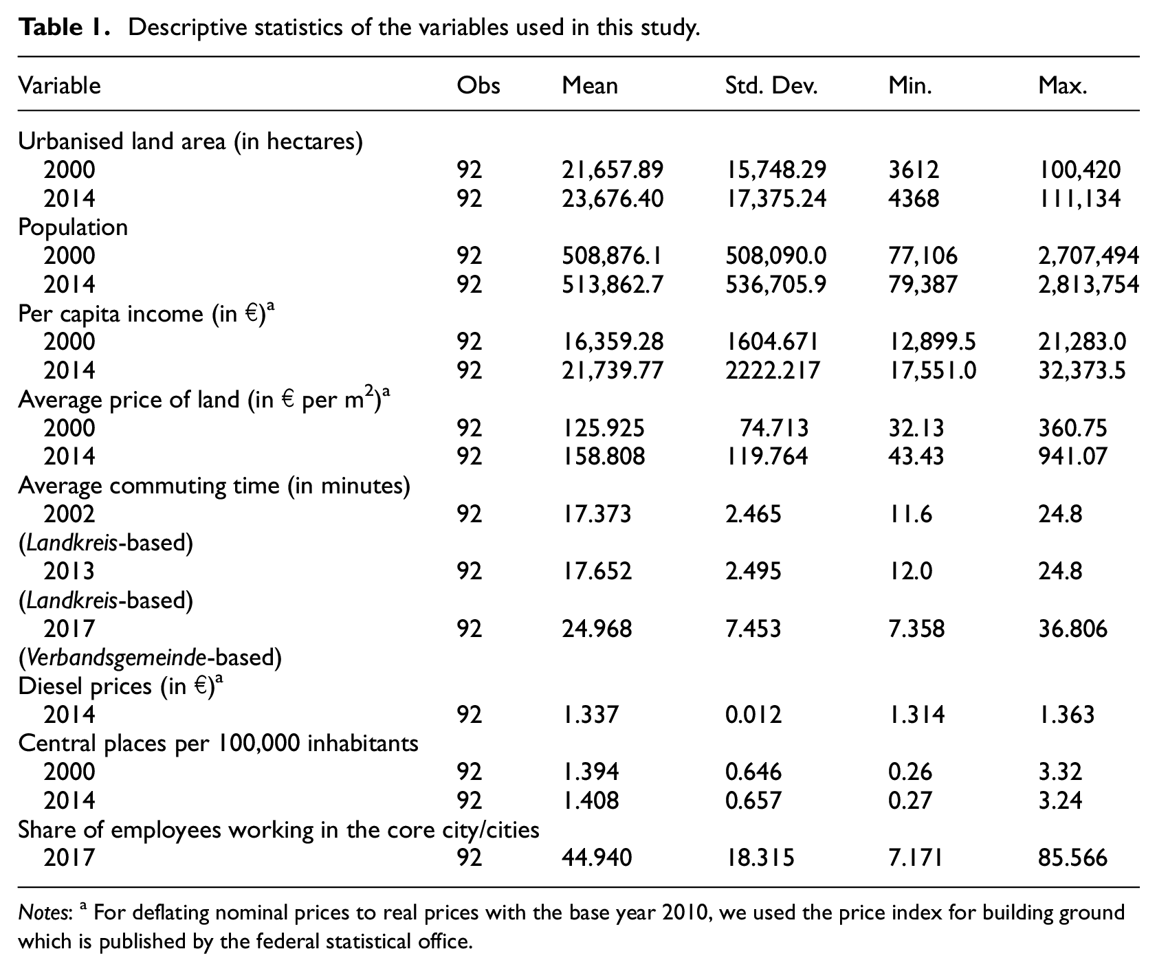
Notes: ^a For deflating nominal prices to real prices with the base year 2010, we used the price index for building ground which is published by the federal statistical office.

We first estimate cross-sectional models separately for two points in time, 2000 and 2014, using urbanised land area as the dependent variable. For 2014, we estimated two models, one where transportation cost is operationalised using average Verbandsgemeinde-based commuting times, and another where transportation cost is operationalised as average diesel prices.

We identified some estimation problems with the standard OLS model due to heteroscedasticity and misspecification. The latter could be due to insufficient acknowledgement of spatial dependence. Thus, we ran some space-related regression diagnostics and concluded, based on (robust) Lagrange Multiplier test statistics, that a spatial error model is more appropriate than standard OLS or a spatial lag model. As our main interest in this article is to test whether or not an augmented version of the AMM model holds for German labour market regions, we did not go further into the details of additional sources of spatial dependence. We therefore employed a robust spatial error model and a Queen’s first order contiguity spatial weights matrix for all years under consideration.²

Second, in order to exploit the balanced panel structure of our data, we perform a panel data estimation using a fixed effects estimator. The primary advantage of a panel approach is that the larger sample size often results in more efficient estimates, particularly if the researcher is interested in understanding the change between two time periods and why different observations behave differently at different time periods. Several previous studies have utilised a panel framework. Examples include McGrath (2005), who estimates the model for 33 cities in the US from 1950 to 1990; Paulsen (2012), who uses urbanised land data from 1980, 1990 and 2000 for 329 metropolitan areas; and Oueslati et al. (2015), who utilise panel data for 282 European cities in 1990, 2000 and 2006.

In addition to comparing the marginal effects of some of the independent variables between the cross-sectional and panel models, we also calculate the elasticities for both models and compare them with elasticities of similar studies.

On the validity of the monocentric city model

Cross-sectional estimates

Table 2 presents the results of the cross-sectional models for the two years (2000 and 2014). Two models were utilised for 2014; the first capitalises on the availability of the average fuel price data for 2014, and the second utilises the fine-grained commuting data available for 2017.

Table 2.

Cross-section estimates of the monocentric model.

	Urbanised land area 2000(using Landkreis data)	Urbanised land area 2014(using diesel prices)	Urbanised land area 2014 (using Verbandsgemeinde data)
Population	0.0317^***	0.0338^***	0.0304^***
Population	(0.000)	(0.000)	(0.000)
Per capita income	−0.453	−0.0450	−0.0483
Per capita income	(0.099)	(0.850)	(0.813)
Avg. price of land (€/m²)	−28.80^***	−21.62^**	−11.99^*
Avg. price of land (€/m²)	(0.000)	(0.002)	(0.046)
Avg. commuting time (2002, 2017)	256.2	-	536.0^***
Avg. commuting time (2002, 2017)	(0.225)		(0.000)
Avg. price of diesel, 2014		31441.9
Avg. price of diesel, 2014	-	(0.401)	-
Central place per 100,000	204.1	342.0	−376.7
Central place per 100,000	(0.700)	(0.614)	(0.457)
East/West dummy	−5978.9^***	−3748.5^*	−2694.7
East/West dummy	(0.000)	(0.019)	(0.198)
Constant	12,049.4^*	−31,635.1	−1655.9
	(0.013)	(0.523)	(0.708)
lambda Constant	0.480^***	0.508^***	0.556^***
lambda Constant	(0.000)	(0.000)	(0.000)
sigma Constant	2980.4^***	3816.2^***	3249.9^***
sigma Constant	(0.000)	(0.000)	(0.000)
Observations	92	92	92
AIC	1759.6	1806.3	1779.1
BIC	1782.3	1829.0	1801.8

Notes: Spatial error model with robust standard errors. p-values in parentheses.

p < 0.05, ^**p < 0.01, ^***p < 0.001.

In all the models, the spatial error coefficient (lambda) was highly significant. Furthermore, in each of the models, coefficients for population and the average price of land were significant and had the expected sign in accordance with the theory. Keeping in mind that urbanised land area is measured in hectares, the population coefficients indicate that, all else being equal, one more resident would be associated with more than 300 m² of additional urbanised land area in 2000 and 2014.³ The difference between the 2000 and 2014 coefficients suggests that the marginal land consumption per new urban resident has remained fairly stable over 14 years and proves quite robust across model specifications. This finding is in contrast with Paulsen (2012), who found that US metropolitan areas saw increasing rates of land consumption per capita over time.

Per capita income was not significant in explaining urban area size in any cross-sectional model specification. This is in contrast to both the theory and the empirical results obtained in US studies that found income to be significant in explaining urbanised area (Brueckner and Fansler, 1983; McGrath, 2005; Paulsen, 2012; Spivey, 2008). The reasons for these counterintuitive results could be that increased demand for housing (and hence urbanised areas) was not realised due to growth management policies and restrictive land use regulation. While there are no such constraints included in the traditional AMM model, they are very much a reality in German metropolitan areas. This is consistent with our hypothesis that German metropolitan regions are less responsive to market forces compared with their US counterparts. In addition, much recent metropolitan population growth has taken place in central areas, especially on brownfield land through infill development (Schmidt et al., 2018). Higher incomes have led to greater housing space consumption, but the effect on urban areal size and spatial structure is less obvious. This trend could be another explanation as to why income is uncorrelated with urban size in our model.

The dummy variable for whether or not a region was located in eastern Germany was significant and negative in nearly all models. The coefficients are quite large, though decreasing over time and losing statistical significance, suggesting a decline in regional differences between eastern and western Germany, a finding that corroborates conclusions elsewhere (Schmidt, 2011; Schmidt et al., 2014). However, metropolitan areas in eastern Germany are underrepresented in our sample, so the reported results should not be overinterpreted.

The number of central places per capita, our proxy to capture polycentricity, was not significant in any of the models, contrary to the findings of Schmidt et al. (2018). That said, the implication that German metropolitan areas are fairly monocentric is in line with Krehl (2015, 2018) and Knapp and Volgmann (2011). Krehl (2018: 90f.) demonstrates that distance to the main employment centre explains between 50% and 75% of the regional employment density pattern in four selected German city regions.

The different proxies for transportation costs proved unreliable. While the average commuting time in 2000 was statistically insignificant, it was significant and positive when using the more fine-grained commuting variable available in 2017. These results are somewhat surprising because the theory suggests that an increase in travelling costs should decrease the urbanised area. However, we are utilising pure travelling times rather than monetary costs, which the AMM model suggests. Thus, we rely on time as a proxy for transportation opportunity cost. The average price of diesel as a true monetary cost for any given distance, which better operationalises the theory behind the monocentric model, is not significant in explaining the urbanised area size. These partly counterintuitive results are similar to other studies that have had difficulty operationalising transportation costs (Brueckner and Fansler, 1983; McGrath, 2005; Oueslati et al., 2015; Spivey, 2008). Paulsen (2012: 564) suggests that the reason is that transportation times in general (and commuting patterns in particular) are endogenous to the model, but some additional discussion as to why fuel price may not be significant is warranted. First, there is very little geographic variation in the fuel prices in Germany to significantly contribute to explaining urban spatial structure. Second, a large number of commuters utilise company cars and therefore are not sensitive to fuel prices; and third, German metropolitan areas are sufficiently reliant on public transit so that the variable fuel prices only have a moderate impact on transportation costs.

The elasticities of urbanised land area with respect to the classic AMM model’s independent variables are presented below. Again, they are based on a spatial error model with robust standard errors. They are evaluated at sample means and suggest elasticities less than unity.

A 1% increase in population in 2000 would increase demand for urbanised land by 0.74%. This result is similar to estimated population elasticities in some of the US studies, in particular McGrath (2005, who reports 0.76%) and Paulsen (2012: 565, who reports 0.62 to 0.635%), but substantially lower than Spivey (2008, who reports 0.91%) and Brueckner and Fansler (1983, who estimate a nearly unitary elasticity). The elasticity of urbanised land area with respect to the average price of land is lower for both points in time than similar estimates by Brueckner and Fansler (1983, −0.231) and Paulsen (2012, ranging from −0.220 to −0.258), but larger than estimates by McGrath (2005, −0.1) and Spivey (2008, −0.03).

In general, the identified statistically significant elasticities (see Table 3) match well with the theoretical predictions from the AMM model. Thus, we conclude that the monocentric city model holds comparatively well for German labour market regions despite the fact that many regions exhibit a rather decentralised and polycentric urban structure.

Table 3.

Cross-section elasticities: Elasticities using the delta method, evaluated at all means.

	Urbanised land area 2000(using Landkreis data)	Urbanised land area 2014(using diesel prices)	Urbanised land area 2014 (using Verbandsgemeinde data)
Population	0.7460^***	0.7332^***	0.6581^***
Population	(0.000)	(0.000)	(0.000)
Per capita income	−0.3430	−0.0413	−0.0442
Per capita income	(0.098)	(0.850)	(0.813)
Avg. price of land (€/m²)	−0.1679^***	−0.1448^**	−0.0801^*
Avg. price of land (€/m²)	(0.000)	(0.002)	(0.041)
Average commuting time (2002, 2017)	0.2060	-	0.5631^***
Average commuting time (2002, 2017)	(0.223)		(0.000)
Avg. price of diesel, 2014		1.7740
Avg. price of diesel, 2014	-	(0.403)	-
Central place per 100,000	0.0132	0.0203	−0.0223
Central place per 100,000	(0.700)	(0.615)	(0.455)
East/West dummy	−0.0120^***	−0.0069^**	−0.0049
East/West dummy	(0.000)	(0.016)	(0.194)
Observations	92	92	92

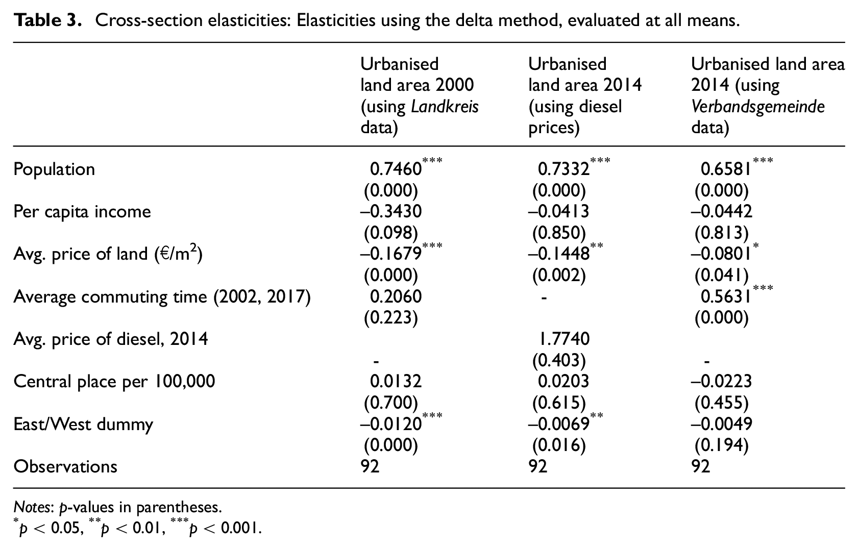
Notes: p-values in parentheses.

p < 0.05, ^**p < 0.01, ^***p < 0.001.

Panel estimation results

In addition to the cross-sectional models, we also estimated our models in a panel framework, a method utilised by similar studies (McGrath, 2005; Oueslati et al, 2015; Paulsen, 2012). The advantage of utilising a panel model is that it is able to fix potential biases that occurred in cross-section models, such as unobserved time-invariant regional characteristics that affect both earlier and later time periods. We utilised a Hausman-type test to compare the appropriateness of using either fixed or random effects estimators. The results indicated that the fixed effects model is preferred. Whereas cross-sectional estimates measure the average behaviour of a ‘typical’ region in either a western or eastern region, the fixed effects panel estimates measure the marginal effect of an explanatory variable on the dependent variable but permitting for region-specific intercepts. The panel data estimation results for the full sample of metropolitan regions are presented in column 2 of Table 4. In addition, we also tested whether the model differed between growing and non-growing regions (for our purposes, non-growing regions include both shrinking regions and regions with unclear development direction). For the classifications of ‘growing’ and ‘non-growing’, we relied on the BBSR, which created a multi-dimensional index incorporating population change, net migration, change in workforce and employment, the rate of unemployment and change in tax incomes, to distinguish growing from shrinking cities (for details, see BBSR, 2015). These results are presented in columns 3 and 4.

Table 4.

Panel estimates of the monocentric model (using xtreg in Stata and the option vce(robust).

	All regions	Growing regions	Non-growing regions
Population	0.0184^***	0.0295^***	−0.0324^***
	(0.007)	(0.000)	(0.000)
Per capita income	0.187^***	0.171^**	0.0700
	(0.000)	(0.001)	(0.209)
Avg. price of land (€/m²)	7.885	3.749	2.919
	(0.054)	(0.187)	(0.687)
Average commuting time (2002, 2013)	2009.8^*	2856.1^**	1472.5^*
	(0.020)	(0.005)	(0.032)
Central place per 100,000	−503.0	2558.2	−2536.4
	(0.820)	(0.327)	(0.427)
Constant	−25,915.2	−50,065.0^**	5717.7
	(0.090)	(0.005)	(0.614)
Observations	184	124	60
Within R ²	0.759	0.833	0.819

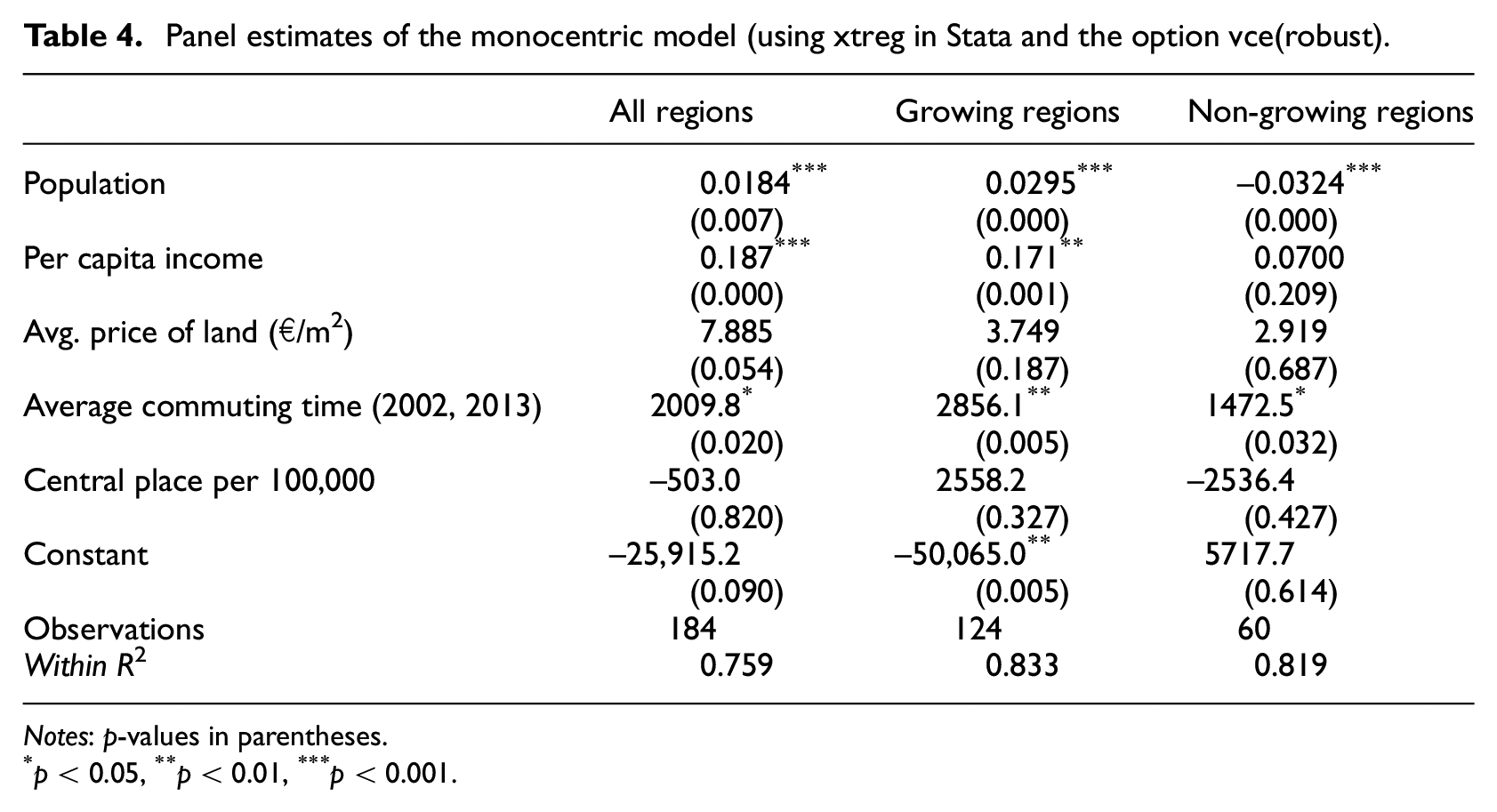
Notes: p-values in parentheses.

p < 0.05, ^**p < 0.01, ^***p < 0.001.

The models perform remarkably well with goodness of fit values of 0.75 and greater, suggesting that the AMM model works well for the entire set of regions. As predicted by the theory, the panel estimated coefficient for population is highly significant and positive. However, it was negative for non-growing regions. This implies that if the population decreases in non-growing cities, the urbanised area will nevertheless increase; this is even greater than the effect of adding an additional person to a growing region. The reasons for this theoretically counterintuitive result could be differences in land use policies and regulatory approaches between growing and non-growing cities. Shrinking cities in particular are more likely to promote development in order to attract new firms and residents (Wiechmann and Pallagst, 2012), while growing cities are more likely to regulate and manage growth. However, the policy dimension is not accounted for in the AMM model and we do not have information in our sample to further examine this issue here.

Unlike the cross-sectional model, per capita income was highly significant, whereas the price of land was not. The reasons for the change in significance could be that the cross-section models suffer from an omitted variable bias that was resolved in the panel specification. It may prove useful to include further (unobserved) region-specific but time-fixed variables into the cross-section models, such as housing preferences or urban labour market capacities, in order to capture this. Interestingly, per capita income ceases to be significant in non-growing regions, but remains significant in growing regions, suggesting that non-growing regions are less responsive to changes in wealth.

Average commuting time is significant for all regions and is positively related to urban area size, a result also in line with the cross-section results but somewhat contradictory to the theory as it suggests that transportation costs negatively affect urban area size. For the panel estimation, we were limited to utilising only the average commuting time variable based on the Landkreise. As mentioned earlier, this could be because the commuting variable does not properly account for all transportation costs, including both opportunity cost of commuting and monetary cost of commuting.

Panel estimated elasticities are presented in Table 5. As with the elasticities for the cross-sectional model, the elasticities for urbanised land area were calculated at sample means.

Table 5.

Panel estimated elasticities of urbanised land area, evaluated at all means using the delta method.

	All regions	Growing regions	Non-growing regions
Population	0.4146^**	0.6835^***	−0.6667^***
	(0.006)	(0.000)	(0.000)
Per capita income	0.1576^***	0.1298^**	0.0765
	(0.000)	(0.001)	(0.198)
Avg. price of land (€/m²)	0.0495^*	0.0241	0.0170
	(0.050)	(0.182)	(0.684)
Avg. commuting time (2002, 2013)	1.5527^*	1.9970^**	1.4748^*
	(0.018)	(0.004)	(0.024)
Central place per 100,000	−0.0311	0.1311	−0.2405
	(0.819)	(0.323)	(0.421)
Observations	184	124	60

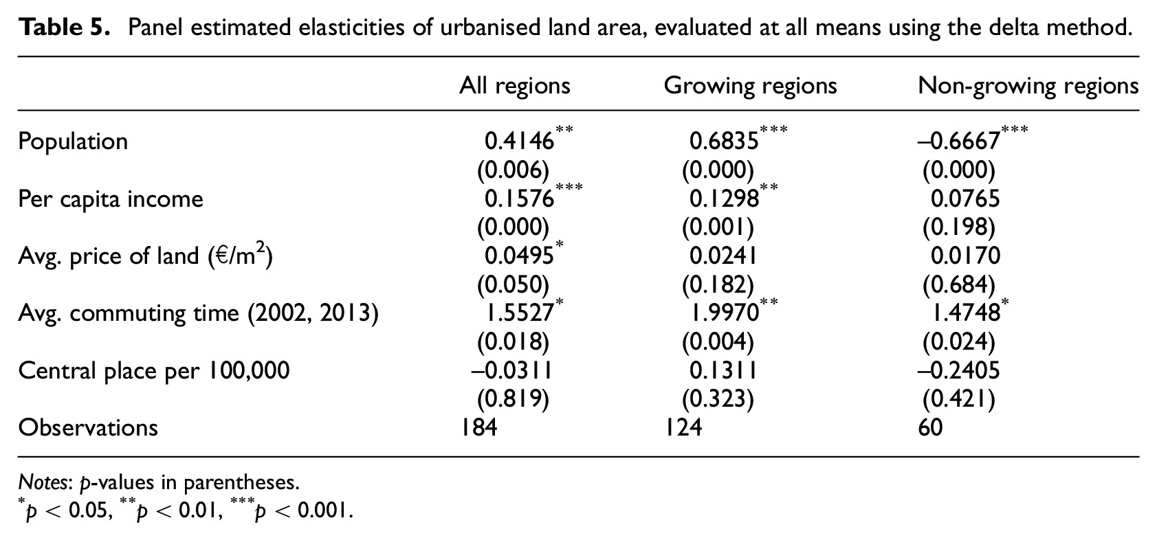
Notes: p-values in parentheses.

p < 0.05, ^**p < 0.01, ^***p < 0.001.

The estimated elasticity of urbanised land with respect to change in population is 0.41 for all regions, which is substantially lower than those estimated by McGrath (2005, 0.76) and Paulsen (2012, 0.8), but greater than that found by Oueslati et al. (2015, 0.288). These relations change if we separate growing and non-growing regions. Growing cities increase in size when population increases, whereas non-growing cities increase in size with falling population. We note an average increase in the urbanised area of 41% if population increases by 1%; this value substantially changes if we separately analyse growing and non-growing labour market regions. Growing regions have similar elasticities to those of US regions (McGrath, 2005; Paulsen, 2012). The percentage changes are almost identical for non-growing regions – it is just the directions that differ – which suggests different strategic orientations and land use policy approaches.

The elasticity of land area with respect to income (0.15) is much lower than the elasticities found by Paulsen (2012, 0.399), McGrath (2005, 0.33) and Brueckner and Fansler (1983, 1.4). Interestingly, the elasticity of income is insignificant for non-growing areas, suggesting that increasing wealth would have no impact on urban area size in declining regions. The elasticity of land prices is significantly positive for the entire sample of regions, but is insignificant if growing and non-growing regions are analysed separately. This finding is in line with our regression analysis, and supports the interpretation that urbanised areas in Germany are less responsive to income increases as compared with the United States, for instance. The elasticity of the polycentricity proxy is insignificant in almost all specifications, suggesting it is not as relevant in explaining urban area size as the other variables.⁴ Average commuting time is significantly positive with values larger than unity, suggesting that urbanised area reacts in an elastic way to commuting time increases. Again, the coefficient’s wrong sign could be due to the measurement issues discussed above.

Conclusion

In this article, we have empirically investigated the explanatory power of the monocentric model in Germany, utilising a unique dataset covering 92 urban labour market regions over two time periods (2000 and 2014), using both cross-sectional and fixed effects panel models. In addition, we calculated elasticities for the determinants of urbanised area. Despite ignoring time-varying aspects of public policy and controlling for changes in institutional and regulatory environments, the monocentric model provides a robust explanation for urbanisation patterns in German metropolitan areas. In addition to applying the model to Germany, and applying a more consistent proxy for transportation costs than earlier studies, this research has made a number of important contributions.

First, similar to earlier results (Schmidt et al., 2018), we found evidence that regional geography does matter. The East/West dummy variable was consistently significant. The coefficient for the dummy variable for the cross-sectional models indicates that, all else being equal, an eastern metropolitan region is associated with an urbanised area that is considerably smaller than one in the west, expressing the different evolution of urbanisation patterns and land use planning systems. The coefficient decreased over time and has not been included in the fixed effects panel model due to its time-invariant nature.

Second, there are a number of points of comparison between our study and US-based studies. Similar to the US studies, the model performed reasonably well, particularly with the overall fit and the performance of the population variable, which were consistently significant and showed the correct sign. In addition, although the significance was more mixed depending on the model, the income and average land price value variables also performed acceptably. We readily note differences in the significance of the income and land price variables between the cross-sectional and the panel specifications. This could be due to the panel model’s ability to better account for omission of unobserved individual and time-fixed effects. The panel model’s result that land prices do not contribute much in explaining urbanised area is not very surprising. We expected the spatial structure of German metropolitan areas to reflect deliberate policy and integrated planning compared with the market forces of their US counterparts. While our empirical results cannot prove this, they suggest that this might be the case. Similar to the US studies, the proxy for transportation costs was unreliable in its effectiveness in explaining urbanisation patterns. This is not necessarily a repudiation of the AMM model, as the operationalisation of the transportation cost variable does not appropriately consider all facets of urban transportation important in Germany, as discussed earlier.

Third, there are some important similarities and differences with previous studies. Our proxy for polycentricity was not significant. This is in contradiction to the findings of Schmidt et al. (2018), who found that central places per capita were consistently significant in explaining urbanisation patterns at the regional level. However, it is in line with Krehl (2018), who finds evidence for the continued monocentric nature of German city regions. Similarly, average price of land was significant for this study, but was not significant according to Schmidt et al. (2018). This is a puzzling difference which could be the result of differences in the units of analysis: the Schmidt et al. (2018) study examined administrative regions, while in this study we were interested in metropolitan regions. These differing results confirm the scalar complexity and multidimensionality of the current urban spatial structure (see also Krehl and Siedentop, 2019), and confirm Agarwal et al. (2012: 440): ‘polycentricity is fully consistent with monocentricity applied locally’.

Finally, our results suggest that the model’s performance also depends on whether a region is growing or non-growing. We found evidence for a growth-oriented development strategy in demographically and/or economically declining regions. Such strategies seek to attract new residents, firms and taxpayers with developable (and often subsidised) land. Future research efforts could explore these issues in greater depth by utilising longer time spans to provide deeper insights into the roles that demographic and economic decline play in ongoing spatial restructuring processes. Along similar lines, considering the role of land use policies would permit a more encompassing view of the validity of the AMM model in the German context.

Footnotes

Declaration of conflicting interests

The author(s) declared no potential conflicts of interest with respect to the research, authorship, and/or publication of this article.

Funding

The author(s) received no financial support for the research, authorship, and/or publication of this article.

ORCID iDs

Stephan Schmidt

Angelika Krehl

Notes

References

Agarwal

Giuliano

Redfearn

(2012) Strangers in our midst: The usefulness of exploring polycentricity. The Annals of Regional Science 48(2): 433–450.

Alonso

(1964) Location and Land Use. Cambridge, MA: Harvard University Press.

BBSR (2015) Wachsende und schrumpfende Städte und Gemeinden in Deutschland. Bonn: BBSR.

Brueckner

(1987) The structure of urban equilibria: A unified treatment of the Muth-Mills model. In: Mills

(ed.) Handbook of Regional and Urban Economics. Amsterdam: North-Holland, pp. 821–845.

Brueckner

Fansler

(1983) The economics of urban sprawl: Theory and evidence on the spatial size of cities. The Review of Economics and Statistics 55: 479–482.

DeSalvo

(2019) The determinants of urban sprawl: Theory and estimation. International Journal of Urban Sciences 23(1): 88–104.

Frenkel

Ashkenazi

(2008) Measuring urban sprawl: How can we deal with it? Environment and Planning B 35: 1–24.

Fujita

Ogawa

(1982) Multiple equilibria and structural transition of non-monocentric urban configurations. Regional Science and Urban Economics 12(2): 161–196.

Gao

Huang

, et al. (2016) How does sprawl differ across cities in China? A multi-scale investigation using nighttime light and census data. Landscape and Urban Planning 148: 89–98.

10.

Glaeser

Kahn

(2004) Sprawl and urban growth. In: Henderson

Thisse

(eds) Handbook of Regional and Urban Economics: Cities and Geography. Amsterdam: Elsevier, pp. 2481–2527.

11.

Gómez-Antonio

Hortas-Rico

(2016) The causes of urban sprawl in Spanish urban areas: A spatial approach. Spatial Economic Analysis 11(2): 219–247.

12.

Knapp

Volgmann

(2011) Neue ökonomische Kerne in nordrhein-westfälischen Stadtregionen: Postsuburbanisierung und Restrukturierung kernstädtischer Räume. Raumforschung und Raumordnung 69(5): 303–317.

13.

Krehl

(2015) Urban spatial structure: An interaction between employment and built-up volumes. Regional Studies, Regional Science 2(1): 290–308.

14.

Krehl

(2018) Urban subcentres in German city regions: Identification, understanding, comparison. Papers in Regional Science 97(1): S79–S104.

15.

Krehl

Siedentop

(2019) Towards a typology of urban centers and subcenters – Evidence from German city regions. Urban Geography 40(1): 58–82.

16.

McGrath

(2005) More evidence on the spatial scale of cities. Journal of Urban Economics 58: 1–10.

17.

McMillen

Smith

(2003) The number of subcenters in large urban areas. Journal of Urban Economics 53(3): 321–338.

18.

Mills

(1972) Studies in the Structure of the Urban Economy. Baltimore, MD: Johns Hopkins University Press.

19.

Müller

Siedentop

(2004) Growth and shrinkage in Germany – Trends, perspectives, and challenges for spatial planning and development. German Journal of Urban Research 43: 14–32.

20.

Muth

(1969) Cities and Housing. The Spatial Pattern of Urban Residential Land Use. Chicago, IL: University of Chicago Press.

21.

Nuissl

Rink

(2003) Urban Sprawl and Post-socialist Transformation: The Case of Leipzig (Germany). Leipzig: UFZ Centre for Environmental Research, UFZ-Berichte 4/2003.

22.

Oueslati

Alvanides

Garrod

(2015) Determinants of urban sprawl in European cities. Urban Studies 52(9): 1594–1614.

23.

Paulsen

(2012) Yet even more evidence on the spatial size of cities: Urban spatial expansion in the US, 1980–2000. Regional Science and Urban Economics 42: 561–568.

24.

Paulsen

(2014) Geography, policy, or market? New evidence on the measurement and causes of sprawl (and infill) in US metropolitan regions. Urban Studies 51(12): 2629–2645.

25.

Schmidt

(2011) Sprawl without growth in eastern Germany. Urban Geography 32(1): 105–128.

26.

Schmidt

Fina

Siedentop

(2014) Post-socialist sprawl: A cross country comparison. European Planning Studies 23(7): 1357–1380.

27.

Schmidt

Siedentop

Fina

(2018) How effective are regions in determining urban spatial patterns? Evidence from Germany. Journal of Urban Affairs 40(5): 639–656.

28.

Siedentop

Fina

(2010) Monitoring urban sprawl in Germany: Towards a GIS-based measurement and assessment approach. Journal of Land Use Science 5(2): 73–104.

29.

Siedentop

Fina

(2012) Who sprawls most? Exploring the patterns of urban growth across 26 European countries. Environment and Planning A 44(11): 2765–2784.

30.

Siedentop

Fina

Krehl

(2016) Greenbelts in Germany’s regional plans – An effective growth management policy? Landscape and Urban Planning 145: 71–82.

31.

Spivey

(2008) The Mills–Muth model of urban spatial structure: Surviving the test of time? Urban Studies 45(2): 295–312.

32.

Stanilov

(2007) The Post-socialist City: Urban Form and Space Transformations in Central and Eastern Europe after Socialism. Berlin: Springer Verlag.

33.

Wassmer

(2006) The influence of local urban containment policies and statewide growth management on the size of United States urban areas. Journal of Regional Science 46(1): 25–65.

34.

Wheaton

(1974) A comparative static analysis of urban spatial structure. Journal of Economic Theory 9(2): 223–237.

35.

Wiechmann

Pallagst

(2012) Urban shrinkage in Germany and the USA: A comparison of transformation patterns and local strategies. International Journal of Urban and Regional Research 36: 261–280.