
Abstract
In this article, we adjust the Kuk randomized response model for collecting information on a sensitive characteristic for increased protection and efficiency by making use of forced “yes” and forced “no” responses. We first describe Kuk’s model and then the proposed adjustment to Kuk’s model. Next, by means of a simulation study, we compare the efficiency of the adjusted Kuk model relative to the pioneer Kuk model while maintaining at least equal protection of respondents.
Introduction
The collection of data on sensitive characteristics from human populations is not an easy task. For example, sensitive questions such as (a) Are you an Alawite? (b) Are you gay? (c) Have you ever molested a child? (d) Have you underreported your income on your tax return? (e) Do you smoke marijuana? (f) Have you ever cheated on an exam? (g) Are you a Baath Party Member? (h) Have you ever been involved in a crime? and so on, are not likely to be responded to honestly by the respondents if asked using direct question survey methods.
The randomized response technique (RRT) was first introduced by Warner (1965) to deal with the problem of estimating the proportion of individuals possessing a sensitive characteristic in a finite population. This technique enables respondents to provide truthful information anonymously on sensitive or highly personal questions without endangering their privacy. His design involves the use of two questions or statements, each of which divides the population into two mutually exclusive and complementary groups (say) A and not-A. In order to estimate π, the proportion of the population in the sensitive group A, each person appearing in a simple random sampling with replacement (SRSWR) sample is given a suitable randomization device. Using the device, the respondent is presented with one of the two statements of the form:
(i) I belong to group A (ii) I do not belong to group A.
The statements (i) and (ii) have known relative frequencies P and (1 − P), respectively, in the randomization device. The respondent answers “yes” or “no” according to the statement randomly selected and to his or her actual status with respect to membership in A, without revealing to the interviewer which statement has been chosen. In this way, the respondent preserves his or her privacy. Note that the true probability of a “yes” answer,

Suppose n* persons in the sample answered “yes” and n – n* answered “no.” An unbiased estimator

The estimator is unbiased if the respondents are persuaded to respond truthfully. Since

Clearly, the first part in equation (3) is the usual binomial variance associated with a direct question and truthful replies by all respondents and the second part is the additional variance due to the randomization device.
Warner (1965) noted that his estimator could assume values outside the closed interval [0, 1]. This drawback was first removed by Singh (1976) by proposing an estimator known as a shrinkage estimator, and later Raghavarao (1978) also made an attempt in this direction and developed a nonlinear biased estimator. Lee, Sedory, and Singh (2013) have pointed out that the Warner (1965) estimator remains an MLE for large sample sizes. They have provided minimum sample sizes that are required by the Warner (1965) estimator to attain values within the unit interval [0, 1]. They also reported that for small sample sizes the modification of the Warner (1965) estimator suggested by Singh (1976) remains valid.
Tracy and Osahan (1999) studied a new partial randomized response strategy in comparison to the Mangat and Singh (1990) model. Mangat and Singh (1994) provide a modified version of the Warner (1965) randomized design where the respondent is free to give an answer in terms of “yes” and “no” either by using a randomized response device or without using it. Singh et al. (1994) have suggested a two-stage RRT to estimate the proportion of population possessing a sensitive attribute. Odumade and Singh (2009) and Singh and Sedory (2011) have investigated a new estimator for estimating the proportion of a sensitive attribute by making use of two decks of cards. There are many models that have been developed and compared with the Warner (1965) model by several researchers, for example, refer to Mangat and Singh (1990), Mangat (1994), Gjestvang and Singh (2006), Barabesi, Diana, and Perri (2013, 2014), Diana, Giordan, and Perri (2013), and Abdelfatah and Mazloum (2014) among others. An extensive review of literature on randomized response sampling can be found in monographs by Chaudhuri (2011) and Chaudhuri and Christofides (2013). Nayak (1994) showed that most of the newly proposed randomized response models as of 1994 are as efficient as the Warner (1965) estimator at equal protection of respondents. We note that many models such as Warner (1965), Mangat and Singh (1990), and Mangat (1994) are special cases of another ingenious model due to Kuk (1990). This motivated the authors to think about trying to improve Kuk’s model from both the protection and efficiency points of views.
Kuk (1990) proposed a randomized response model that makes use of two randomization devices. The first randomization device, R 1 (say), has two possible outcomes, say a deck of cards each card bearing one of two possible questions: (i) Are you a member of group A? and (ii) Are you a member of group Ac ? with known probabilities θ1 and (1 − θ1), respectively. The second randomization device, R 2 (say), has the same two possible outcomes, say a deck of cards, each card bearing one of two possible questions: (i) Are you a member of group Ac ? and (ii) Are you a member of group A? With known probabilities θ2 and (1 – θ2), respectively. Assume that an SRSWR sample of n respondents is selected from the population of interest. Each respondent selected in the sample is provided with both randomization devices, R 1 and R 2, along with instructions on how to make use of these devices. Each respondent is also given the instruction that, if he or she belongs to the sensitive group A, then he or she should make use of the first randomization device R 1, while if he or she belongs to the nonsensitive group Ac , then he or she should make use of the second randomization device R 2, without disclosing to which group, A or Ac , he or she belongs. That is, the choice between the two randomization devices R 1 and R 2 is being made by the interviewee unobserved by the interviewer. Hence, the privacy of the respondent is maintained.
The true probability of a “yes” answer

and the maximum likelihood and unbiased estimator of π is given by:

where

Note that if θ1 = P and θ2 = (1 – P), then Kuk’s randomized response model reduces to the Warner (1965) model. If θ1 = 1 and θ2 = (1 – P), then Kuk’s model reduces to the Mangat (1994) model, and so on.
Adjusted Kuk’s Randomized Response Model
We consider selecting an SRSWR sample of n respondents from the given population of interest. Each respondent in the sample of n respondents is provided with two randomization devices, D
1 and D
2. The randomization device D
1 consists of a deck of cards, each card bearing one of two types of statements: (i) Use randomization device F
1 and (ii) Use randomization device

Flow chart of the adjusted Kuk randomized response model.
In the adjusted Kuk model, the probability of a “yes” answer is given by:
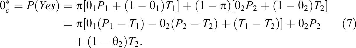
Let X be the number of observed “yes” answers in the SRSWR sample of n respondents. Obviously
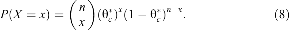
The log likelihood function is given by:

On setting
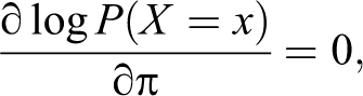
we get

as the MLE of the probability of a “yes” answer.
By the method of moments, we have the following theorem.

where


Hence the theorem.

Measures of Respondents’ Privacy Protection
Following Lanke (1975), we use his measure of protection of respondents, for Kuk’s and the proposed models defined as follows. The conditional probability in Kuk’s model that a respondent reporting “yes” also belongs to the sensitive group A is given by:

The conditional probability in Kuk’s model that a respondent reporting “no” also belongs to the sensitive group A is given by:
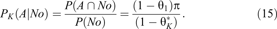
The least protection (or greatest incrimination) of a respondent reporting either “yes” or “no” while experiencing Kuk’s model is given by:

The conditional probability that a respondent reporting “yes” with the adjusted Kuk randomized response model also belongs to the sensitive group A is given as follows:

The conditional probability that a respondent reporting “no” with the adjusted Kuk randomized response model also belongs to the sensitive group A is given by:

The least protection of a respondent reporting either “yes” or “no” while experiencing the adjusted Kuk randomized response model is given by:

Comparison of the Models
We define the percentage relative protection (RP) of the adjusted Kuk randomized response model with respect to Kuk’s randomized response model as:

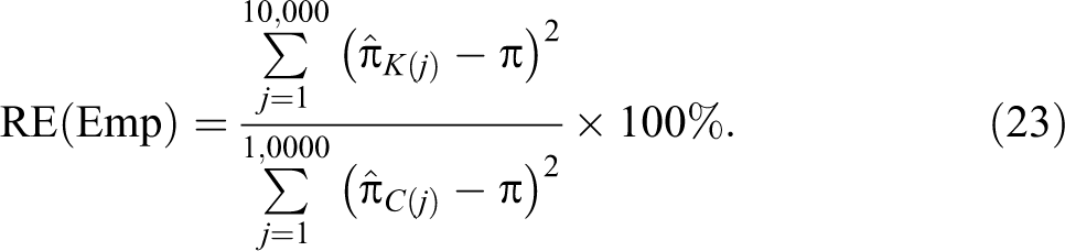
We also define the percentage relative efficiency (RE) of the adjusted Kuk randomized response model with respect to the pioneer Kuk model as:

For given values of θ1, and θ2 in Kuk’s model, we did a grid search for different choices of values of P 1, P 2, T 1, and T 2 such that

The Statistical Analysis System (SAS) codes used to produce results shown in Figure 2 are given in Supplementary Appendix A. Search results, given in Figure 2, demonstrate that for the given choice of parameters in Kuk’s model (say θ1 = 0.7 and θ2 = 0.2), and for each choice of π where 0.1 ≤ π ≤ 0.9 taken with a step of 0.1 there exists a choice of parameters P 1, P 2, T 1 and T 2 where both criteria are met. One observation that can be made from Figure 2 is that if π is close to 0, then values of RP may be notably higher than 100% in many situations, but when π is close to 0.9, then the value of RP does not differ very much from 100%. This means that if a characteristic is very sensitive and does not occur often in the population of interest, then it is feasible to construct a randomized response model that is more protective than its competitors and more efficient, but that if the prevalence of the sensitive characteristic across the population is great, then it is difficult to differentiate between the two randomized response models on the basis of privacy protection. To investigate these situations in more detail, we note that there were 1,935 cases where both the criterions are met. We provide in Tables 1 and 2 the descriptive statistics of the percentage RP and percentage RE for a range of values of the parameter of interest, 0.1 ≤ π ≤ 0.9 with a step of 0.1.
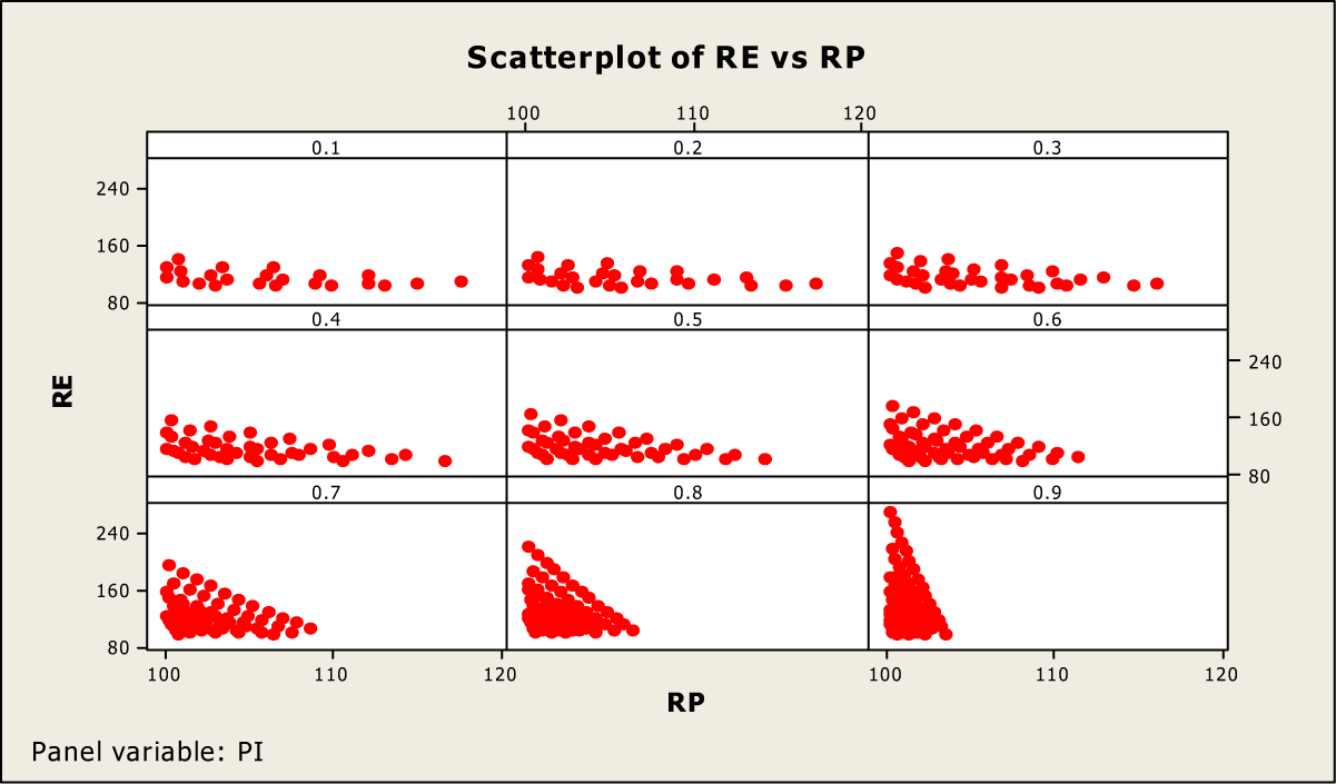
Relative efficiency (RE) versus relative protection (RP) for 0.1 ≤ π ≤ 0.9 with different choice of other parameters 0.1 ≤ P 1, P 2, T 1, T 2 ≤ 0.9, θ1 = 0.7, and θ2 = 0.2.
Descriptive Statistics of the Percentage Relative Protection (RP).
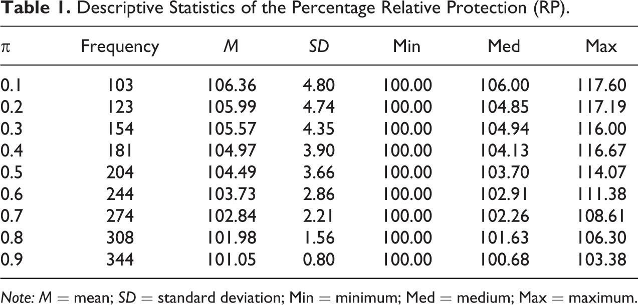
Note: M = mean; SD = standard deviation; Min = minimum; Med = medium; Max = maximum.
Descriptive Statistic of the Percentage Relative Efficiency (RE).
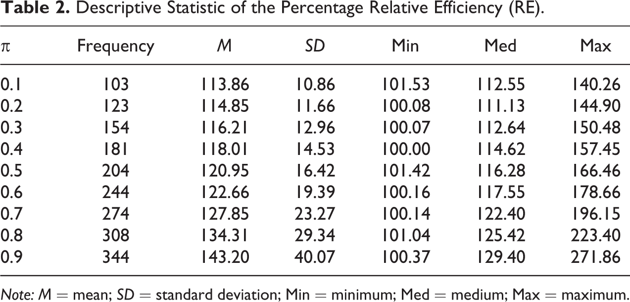
Note: M = mean; SD = standard deviation; Min = minimum; Med = medium; Max = maximum.
We discuss these tables as follows: For π = 0.1, there were 103 combinations of P 1, P 2, T 1, and T 2 and for the given choice of θ1 = 0.7 and θ2 = 0.2 with RE > 100 and RP ≥ 100. Among these, the percentage RP of the proposed adjusted forced randomized response model ranged between 100.00% and 117.60% while the percentage RE values ranged from 101.53% to 140.26%. For π = 0.2, there were 123 combinations of P 1, P 2, T 1, and T 2 where RE > 100 and RP ≥ 100. Among these, the percentage RP of the proposed model ranged between 100.00% and 117.19% while the percentage RE values ranged between 100.08% and 144.90%. For π = 0.1, the median RP among the 103 values was 106.00% with a median RE of 112.55%. The mean RP was 106.36% with a standard deviation (SD) of 4.80%, and the mean RE was 113.86% with an SD of 10.86%. In the same way, the rest of the results in Tables 1 and 2 can be interpreted. Note that the mean and median values of RP are decreasing functions of π as shown in Table 1. For this reason, the percentage RE results are not symmetric around the value of π = 0.5. In other words, the mean percentage RE value for π = 0.1 is not the same as the value of mean percentage RE for π = 0.9.
In Figure 3, we provide four scatter plots showing the values of P 1, P 2, T 1, and T 2 for the fixed values of θ1 = 0.7 and θ2 = 0.2, and for all values of 0.1 ≤ π ≤ 0.9 with a step of 0.1. A close look at Figure 3 indicates that the value of P 1 remains either close to zero or close to 1, there seems to be no restriction on the choice of values of P 2, and T 1, but the value of T 2, the value of T 1 should also not be close to 0.5 if π = 0.5.
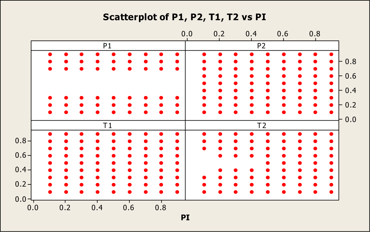
Different choices of other parameters 0.1 ≤ P 1, P 2, T 1, T 2 ≤ 0.9 for θ1 = 0.7, θ2 = 0.2, and 0.1 ≤ π ≤ 0.9.
Thus, based on Figure 3, an investigator could make a choice of parameters P 1, P 2, T 1, and T 2, such that at least equal protection and more efficiency is expected from the adjusted Kuk randomized response model than from the original Kuk model. Similar results are observed for other practicable choice of parameters θ1 and θ2, but we have reported results only for the choice of θ1 = 0.7 and θ2 = 0.2. Other results can easily be produced by executing the provided SAS codes.
In Comparison of the Models section, we compared the final variance expressions of the two estimators for better than equal protection. In the Simulation Study Close to a Real Survey section, we perform a simulation study that can be considered very close to a real survey data set collected using the adjusted Kuk model and the pioneer Kuk model.
Simulation Study Close to a Real Survey
In this section, we used synthetic responses from respondents by using two different models. We explain this simulation procedure as follows: For θ1 = 0.7 and θ2 = 0.2, we compute the probability of “Yes” answer
In addition, we computed the percentage RP of the adjusted Kuk model with respect to the pioneer Kuk model for the adjusting parameters given previously as P 1 = 0.90, P 2 = 0.20, T 1 = 0.90, and T 2 = 0.35. The results are very encouraging in favor of the adjusted Kuk model. The FORTRAN codes used in the simulation study are provided in Supplementary Appendix A.
A summary of the raw results obtained in Supplementary Table A1 is given in Tables 3 and 4 for different levels of value of π.
Summary Statistics of the Percentage RE(Emp) Values.
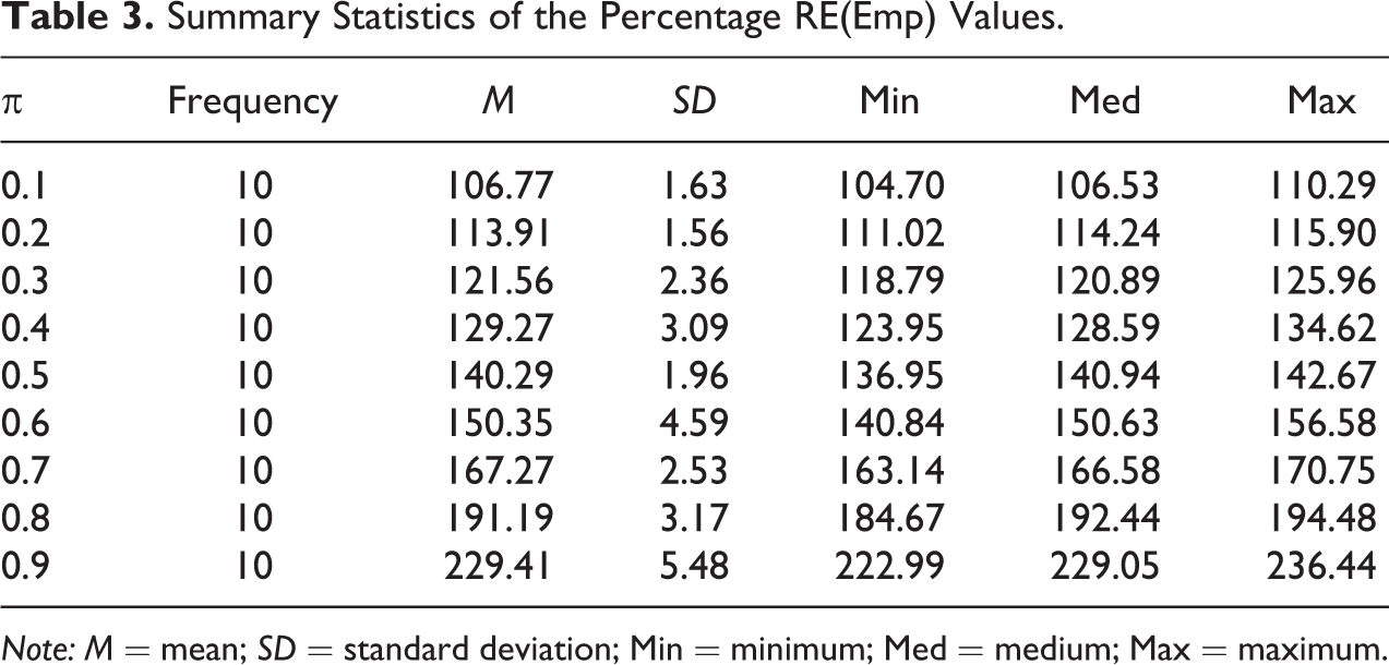
Note: M = mean; SD = standard deviation; Min = minimum; Med = medium; Max = maximum.
The Percentage RP Values for Each Level of π.
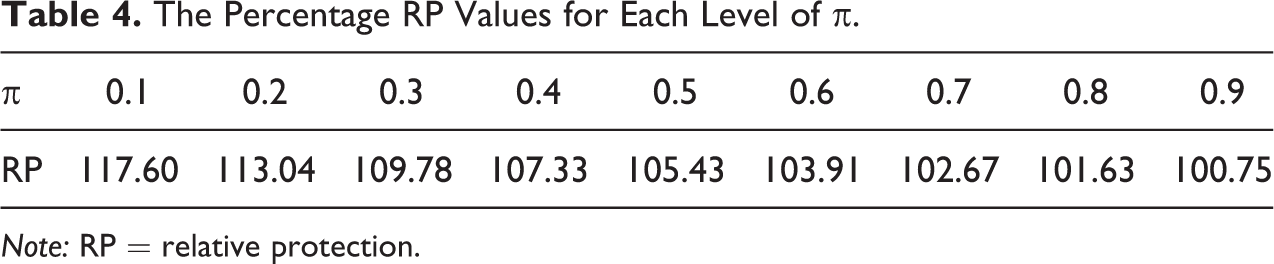
Note: RP = relative protection.
When we compared the true variances then the percentage RE value is free from the value of sample size, but Table 3 shows that there could be slight variation in the percentage RE(Emp) values. For example, if π = 0.1, then the RE(Emp) value ranges from 104.70% to 110.29% as the sample size varies from 100 to 1,000 with a step of 100. The mean RE(Emp) value is 106.77% with an SD of 1.63%, and median value is 106.53%. For π = 0.2, the minimum value of the RE(Emp) was 111.02%, maximum was 115.90% with a median efficiency of 114.24%, and the mean value of 113.91% with an SD of 1.56%. In the same way, the rest of the table can be interpreted. Table 4 reports the percentage RP value for each value of π. The RP is 117.60% if π is 0.1; 113.04% if π is 0.2; and it reduces to 100.75% if π is 0.9.
For another view of the results obtained from the simulation study, we give a few pictorial representations in the scatterplots subsequently.
Figure 4 shows that if the sample size is small, say less that 500, then there is a possibility that the pioneer Kuk estimate can take an inadmissible values if π is either close to zero or close to 1.
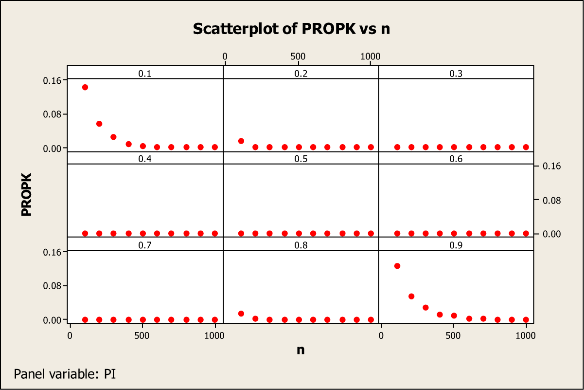
Proportion (PROPK) of inadmissible estimates with Kuk’s pioneer model.
Figure 5 also shows a similar trend for the adjusted Kuk model, in that, if the value of π is close to 0 or 1, then the estimate from the adjusted Kuk model can also take on inadmissible values in the case of small sample sizes, say less than 500. However, the proposed model goes outside the admissible range much less often than Kuk’s model according to Supplementary Table A1 (see Appendix A). Thus, a minimum sample of size of 500 respondents is recommended if an investigator expect the value of π to be close to either 0 or 1. Figure 6 has been devoted to investigating the relationship between the RE(Emp) and RP values for different values of π. The vertical bars for each value of π in the range 0.1 to 0.9 indicate that there is no change in the value of RP but that there is slight change in the percentage RE(Emp) values as the sample size varies from 100 to 1,000, which is consistent with results in Tables 3 and 4.
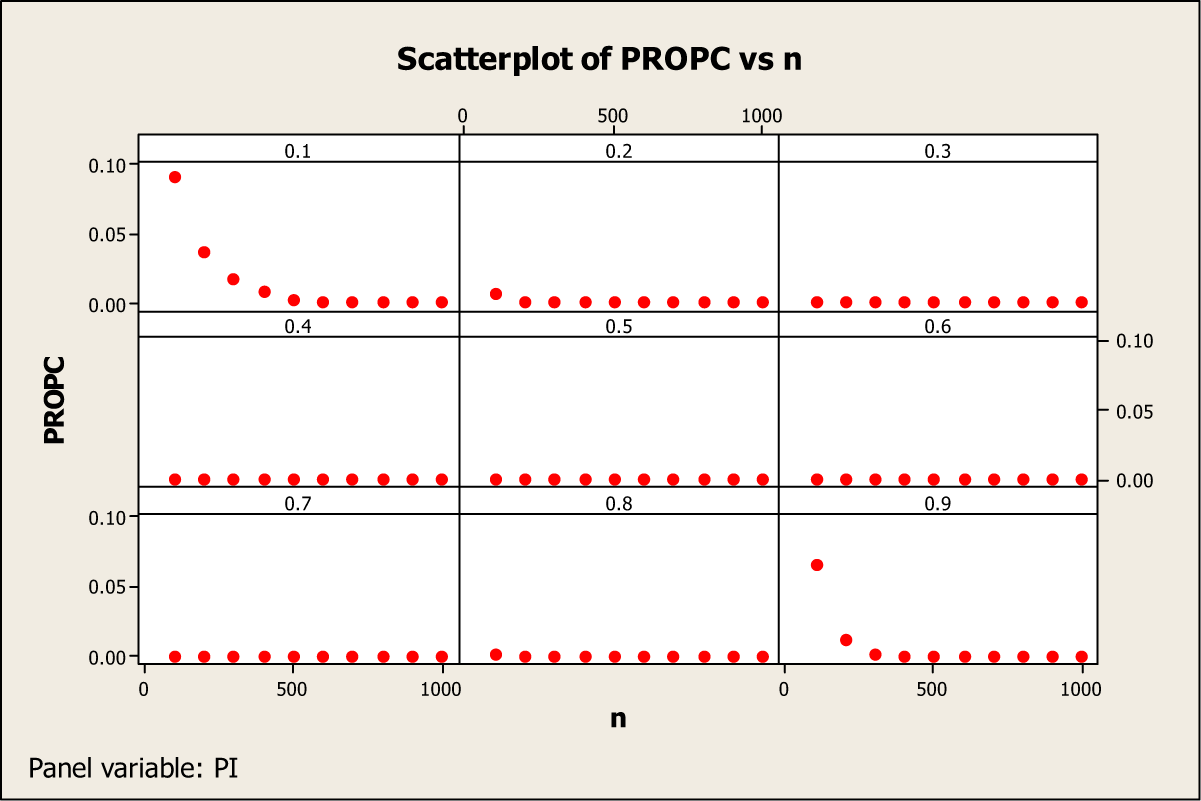
Proportion (PROPC) of inadmissible estimates with Kuk’s adjusted model.
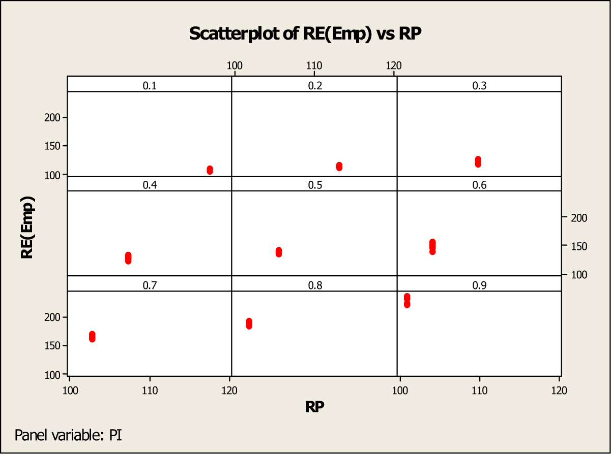
RE(Emp) versus RP for each level of the sensitive attribute.
Figure 7 confirms that due to simulated synthetic 10,000 data values, the value of RE(Emp) changes for each level of value of π as the sample size changes from 100 to 1,000, and this variation is reflected in the SD values of the mean RE(Emp). Also there is no obvious pattern in the variation of RE(Emp) with n, for any of the values of π.
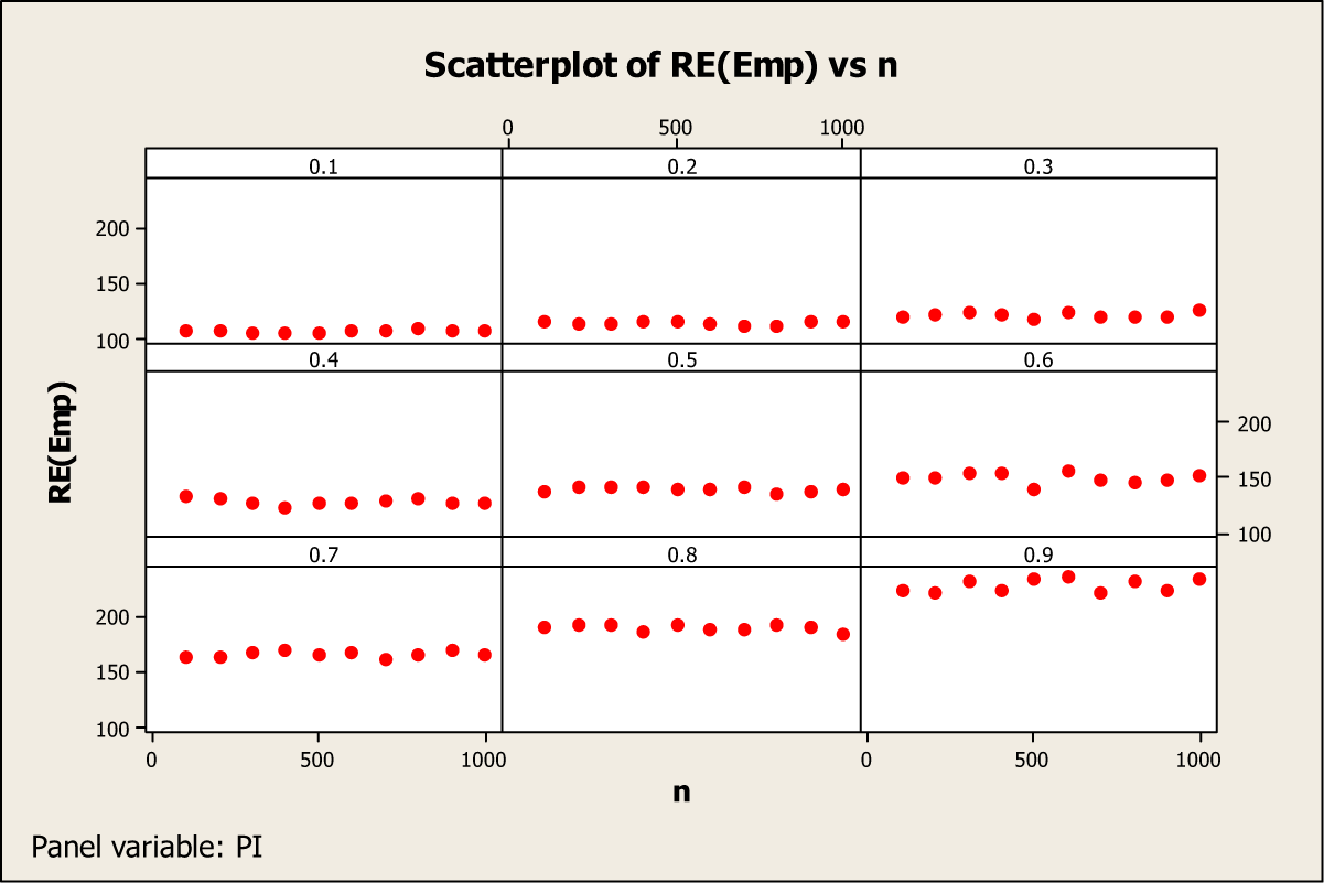
RE(Emp) versus sample size (n) for different values of π.
Figure 8 is an attempt to illustrate the simultaneous effect of the value of level of the sensitive characteristic π and the sample size n on the value of RE(Emp).

RE(Emp) versus sample size (n) versus values of π.
We fit a liner model to predict the percentage RE(Emp) value based on a good guess of the value of π as given as follows:

Conclusion
In this article, we conclude that forced “yes” and forced “no” answers can be used to adjust Kuk randomized response model for increasing both the respondents’ protection and the efficiency of the Kuk model without increasing any cost of the survey.
Footnotes
Acknowledgment
The authors would like to thank Editor Prof. Christopher Winship, Editorial Assistant Genevieve Butler, and three learned referees for their very valuable and critical comments on the original version of this article.
Declaration of Conflicting Interests
The author(s) declared no potential conflicts of interest with respect to the research, authorship, and/or publication of this article.
Funding
The author(s) received no financial support for the research, authorship, and/or publication of this article.