Alternative Methods to Make Efficient Use of Two Decks of Cards in Randomized Response Sampling

Abstract

In this article, alternative randomized response models are proposed, which make use of sum of quantitative scores generated from two decks of cards being used in a survey. The proposed methods are compared to the Odumade and Singh and Singh and Grewal models through a simulation study. It is shown that the modified methods can be used more efficiently than those both models.

Keywords

randomized response technique estimation of proportion relative efficiency

In this article, we first discuss the efficient use of two decks of cards introduced by Odumade and Singh (2009). They showed that a randomized response model based on two decks can easily be adjusted to be more efficient than the Warner (1965), Mangat and Singh (1990), and Mangat (1994) methods by selecting appropriate parameters for their randomization device. The collection of data through personal interview surveys on sensitive issues such as induced abortions, drug abuse, and family income is a serious issue; see, for example, Fox and Tracy (1986), Kerkvliet (1994), Chaudhuri (2011), Chaudhuri and Christofides (2013), Su, Sedory, and Singh (2015), and Fox (2016). Warner (1965) considered the case where the respondents in a population can be divided into two mutually exclusive groups: one group with stigmatizing/sensitive characteristic A and the other group without it. For estimating π, the proportion of respondents in a population belonging to the sensitive group A, a simple random sampling with replacement (SRSWR) sample s of n respondents is selected, from the population. For collecting information on a sensitive characteristic, Warner (1965) made use of a randomization device. One such device could be a deck of cards with each card having one of the following two mutually exclusive statements:

(i) “I belong to group A” and (ii) “I do not belong to group A”

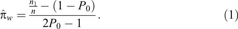
The statements (i) and (ii) occur with relative frequencies P ₀ and (1 − P ₀), respectively, in the deck. Each respondent in the sample s is asked to select a card at random from the well-shuffled deck. Without showing the card to the interviewer, the interviewee answers the question, “Is the statement true for you?” Then the number of people n ₁ that answer “yes” is binomially distributed with parameters $P_{0} π + (1 - P_{0}) (1 - π)$ and n. For large sample size n (see Lee, Sedory, and Singh 2013), the maximum likelihood estimator of π exists for $P_{0} \neq 0.5$ and is given by:

{\hat{π}}_{w} = \frac{\frac{n_{1}}{n} - (1 - P_{0})}{2 P_{0} - 1} .

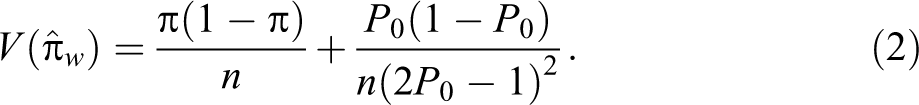
The estimator ${\hat{π}}_{w}$ is an unbiased estimator for π, and the variance of the estimator ${\hat{π}}_{w}$ is given by:

V ({\hat{π}}_{w}) = \frac{π (1 - π)}{n} + \frac{P_{0} (1 - P_{0})}{n {(2 P_{0} - 1)}^{2}} .

Mangat and Singh (1990) suggested a two-stage randomized response model. In the first stage, each respondent is requested to use a randomization device, $R_{1}^{*}$ , such as a deck of cards with each card bearing one of the following two mutually exclusive statements:

(i) “I belong to group A” and (ii) “Go to the randomization device $R_{2}^{*}$ .”

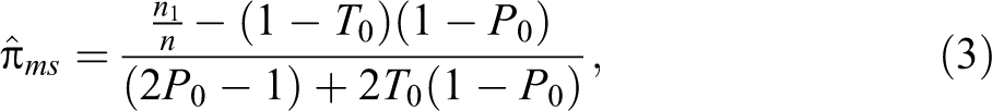
The statements (i) and (ii) occur with relative frequencies T ₀ and (1 − T ₀), respectively, in the first randomization device, $R_{1}^{*}$ . In the second stage, if directed by the outcome of $R_{1}^{*}$ , the respondent is requested to use the second randomization device, $R_{2}^{*}$ , which is the same as the Warner (1965) device. Under the two-stage randomized response model, an unbiased estimator of the population proportion π is given by:

{\hat{π}}_{m s} = \frac{\frac{n_{1}}{n} - (1 - T_{0}) (1 - P_{0})}{(2 P_{0} - 1) + 2 T_{0} (1 - P_{0})},

with variance:

V ({\hat{π}}_{m s}) = \frac{π (1 - π)}{n} + \frac{(1 - P_{0}) (1 - T_{0}) [1 - (1 - P_{0}) (1 - T_{0})]}{n {(2 P_{0} - 1) + 2 T_{0} (1 - P_{0})}^{2}} .

Mangat (1994) considered another randomized response model where each respondent selected in the sample s is requested to report “yes” if he or she belongs to the sensitive group A, otherwise he or she is instructed to use the Warner (1965) device. For this model, an unbiased estimator of the population proportion π is given by:

{\hat{π}}_{m} = \frac{\frac{n_{1}}{n} - (1 - P_{0})}{P_{0}},

with variance given by:

V ({\hat{π}}_{m}) = \frac{θ_{m} (1 - θ_{m})}{n P_{0}^{2}},

where $θ_{m} = π + (1 - π) (1 - P_{0})$ . The Mangat (1994) model is more efficient than both the Warner (1965) and Mangat and Singh (1990) models. We note that the Mangat (1994) model has been improved by Gjestvang and Singh (2006) by adjusting the device parameters.

Kuk (1990) proposed a randomized response model that makes use of two randomization devices. The first randomization device, R ₁ (say) has two possible outcomes, say a deck of cards each card bearing one of two possible questions: (i.) “Are you a member of group A?” and (ii) “Are you a member of group A^c ?” with known probabilities θ₁ and (1 − θ₁), respectively. The second randomization device, R ₂ (say), has the same two possible outcomes, say a deck of cards, each card bearing one of two possible questions: (i) “Are you a member of group A^c ?” and (ii) “Are you a member of group A?” with known probabilities θ₂ and (1 − θ₂), respectively. Assume that an SRSWR sample of n respondents is selected from the population of interest. Each respondent selected in the sample is provided with both randomization devices, R ₁ and R ₂, along with instructions on how to make of use of these devices. Each respondent is also given the instruction that, if he or she belongs to the sensitive group A, then he or she should make use of the first randomization device R ₁, while if he or she belongs to the nonsensitive group A^c , then he or she should make use of the second randomization device R ₂, without disclosing to which group, A or A^c , he or she belongs. That is, the choice between the two randomization devices R ₁ and R ₂ is being made by the interviewee unobserved by the interviewer. Hence, the privacy of the respondent is maintained.

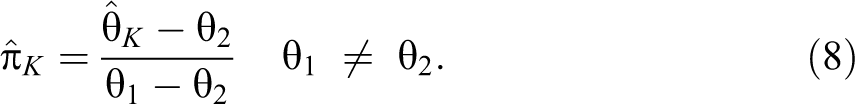
The true probability of a yes answer θ _K is given by:

θ_{K} = π θ_{1} + (1 - π) θ_{2}

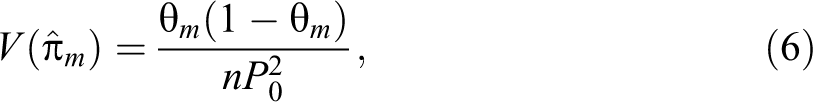
and the maximum likelihood and unbiased estimator of π is given by:

{\hat{π}}_{K} = \frac{{\hat{θ}}_{K} - θ_{2}}{θ_{1} - θ_{2}} θ_{1} \neq θ_{2} .

The variance of the estimator ${\hat{π}}_{K}$ is given by:

V ({\hat{π}}_{K}) = \frac{θ_{K} (1 - θ_{K})}{n {(θ_{1} - θ_{2})}^{2}} .

Note that if θ₂ = (1 − θ₁), then the Kuk’s randomized response model reduces to the Warner (1965) model. If θ₁ = 1 and θ₂ = (1 − P), then the Kuk’s model reduces to the Mangat (1994) model, and so on. Recently, Singh and Grewal (2013) proposed a randomized response model in which each respondent selected in the sample s is provided with two decks of cards in the same way as in the Kuk (1990) model. In the first deck of cards, let $θ_{1}^{*}$ be the proportion of cards with the statement, “I belong to group A” and $(1 - θ_{1}^{*})$ be the proportion of cards with the statement, “I do not belong to group A.” In the second deck of cards, let $θ_{2}^{*}$ be the proportion of cards with the statement, “I do not belong to group A” and $(1 - θ_{2}^{*})$ be the proportion of cards with the statement, “I belong to group A.” Up to here, it is same as the Kuk (1990) randomized response device. Now in the proposed model, if a respondent belongs to group A, he or she is instructed to draw cards, one by one with replacement, from the first deck of cards until he or she gets the first card bearing the statement of his or her own status, and is then requested to report the total number of cards, say X, drawn. If a respondent belongs to group A^c , he or she is instructed to draw cards, one by one using with replacement, from the second deck of cards until he or she gets the first card bearing the statement of his or her own status, and is then requested to report the total number of cards, say Y, drawn. Obviously, $X \sim G (θ_{1}^{*})$ and $Y \sim G (θ_{2}^{*})$ , that is, X and Y follow geometric distributions with parameters $θ_{1}^{*}$ and $θ_{2}^{*}$ , respectively, because cards are drawn based on with replacement sampling. Let Z_i be the number of cards reported by the ith respondent, then Singh and Grewal (2013) proposed an unbiased estimator of the population proportion π given by:

{\hat{π}}_{S G} = \frac{\frac{θ_{1}^{*} θ_{2}^{*}}{n} \sum_{i = 1}^{n} Z_{i} - θ_{1}^{*}}{θ_{2}^{*} - θ_{1}^{*}}, θ_{1}^{*} \neq θ_{2}^{*} .

The variance of the estimator ${\hat{π}}_{SG}$ is given by:

V ({\hat{π}}_{SG}) = \frac{π (1 - π)}{n} + \frac{θ_{2}^{* 2} (1 - θ_{1}^{*}) π + θ_{1}^{* 2} (1 - θ_{2}^{*}) (1 - π)}{n {(θ_{2}^{*} - θ_{1}^{*})}^{2}} .

Now, we discuss an efficient use of two decks of cards proposed by Odumade and Singh (2009).

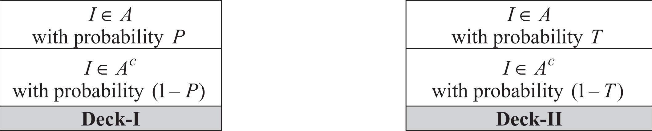
In Odumade and Singh (2009) model, each respondent in an SRSWR sample of n is provided with two decks of cards marked as Deck I and Deck II as shown in Figure 1.

Figure 1.

Two decks of cards.

Each respondent is requested to draw two cards simultaneously, one card from each deck of cards, and read the statements in order. The respondent first matches his or her status with the statement written on the first deck of cards and then he or she matches his or her status with the statement written on the second deck of cards. Let π be the true proportion of respondents in the population that possesses the characteristic A.

Consider a situation that the selected respondent belongs to group A: Now, if he or she draws first card with statement “ $I \in A$ ” (with probability P) from the first deck and a second card with statement “ $I \in A$ ” (with probability T) from the second deck, then he or she would report: (Yes, Yes).

Consider another situation where the selected respondent belongs to group A^c : Now if he or she draws first card with statement “ $I \in A^{c}$ ” (with probability (1 − P)) from the first deck and second card with statement “ $I \in A^{c}$ ” (with probability (1 − T)) from the second deck, then he or she would also report: (Yes, Yes). Thus, the response (Yes, Yes) can come from both types of respondents, these belonging either to group A or to A^c , and hence their privacy will be maintained. The probability of getting a (Yes, Yes) response is given by:

P (Yes,Yes) = θ_{11} = P T π + (1 - P) (1 - T) (1 - π) .

Now consider a situation where the selected respondent belongs to group A: Now if he or she draws first card with statement “ $I \in A$ ” (with probability P) from the first deck and second card with statement “ $I \in A^{c}$ ” (with probability (1 − T)) from the second deck, then he or she would report: (Yes, No).

Again consider another situation where the selected respondent belongs to group A^c : Now if he or she draws first card with statement “ $I \in A^{c}$ ” (with probability (1 − P)) from the first deck and second card with statement “ $I \in A$ ” (with probability T) from the second deck, then he or she would also report: (Yes, No). Thus, the response (Yes, No) can come from both types of respondents, those belonging either to the group A or to A^c , and hence their privacy will not be disclosed. The probability of getting (Yes, No) response is given by:

P (Yes,No) = θ_{10} = P (1 - T) π + (1 - P) T (1 - π) .

Similarly, there are two ways to obtain each of the responses (No, Yes) and (No, No), one from those belonging to A and the other from those not in A. The corresponding probabilities are given by:

P (No,Yes) = θ_{01} = (1 - P) T π + P (1 - T) (1 - π),

and

P (No,No) = θ_{00} = (1 - P) (1 - T) π + P T (1 - π) .

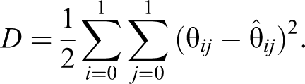
Let ${\hat{θ}}_{11} = n_{11} / n$ , ${\hat{θ}}_{10} = n_{10} / n$ , ${\hat{θ}}_{01} = n_{01} / n$ , and ${\hat{θ}}_{00} = n_{00} / n$ be the observed proportions of (Yes, Yes), (Yes, No), (No, Yes), and (No, No) responses. Odumade and Singh (2009) defined the least square distance between the observed proportions and the true proportions as:

D = \frac{1}{2} \sum_{i = 0}^{1} \sum_{j = 0}^{1} {(θ_{i j} - {\hat{θ}}_{i j})}^{2} .

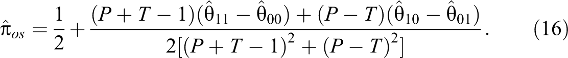
Odumade and Singh (2009) decided to choose as estimator, that value of $\hat{π}$ , such that the least squared distance D is minimum. By setting $\frac{\partial D}{\partial π} = 0$ and solving for π, an unbiased estimator of the population proportion π is given by:

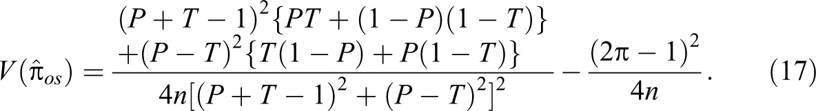
{\hat{π}}_{o s} = \frac{1}{2} + \frac{(P + T - 1) ({\hat{θ}}_{11} - {\hat{θ}}_{00}) + (P - T) ({\hat{θ}}_{10} - {\hat{θ}}_{01})}{2 [{(P + T - 1)}^{2} + {(P - T)}^{2}]} .

The variance of the estimator ${\hat{π}}_{o s}$ is given by:

V ({\hat{π}}_{o s}) = \frac{\begin{array}{l} {(P + T - 1)}^{2} {P T + (1 - P) (1 - T)} \\ + {(P - T)}^{2} {T (1 - P) + P (1 - T)} \end{array}}{4 n {[{(P + T - 1)}^{2} + {(P - T)}^{2}]}^{2}} - \frac{{(2 π - 1)}^{2}}{4 n} .

Note that if T = P = P ₀ (say), the variance of the estimator ${\hat{π}}_{o s}$ in equation (17) becomes:

V {({\hat{π}}_{o s})}_{P = T = P_{0}} = \frac{π (1 - π)}{n} + \frac{P_{0} (1 - P_{0})}{2 n {(2 P_{0} - 1)}^{2}} = V {({\hat{π}}_{w})}_{q = 2},

which is same variance as if each respondent were requested to use the Warner (1965) device twice. A detailed review on recent randomized response sampling techniques can be found in Fox (2016), Johnson (2014), Chaudhuri and Christofides (2013), Chaudhuri (2011), and Singh (2003).

In the present article, let us assume we have two decks of cards as in the Odumade and Singh (2009) model. Further assume that the cards bearing the statement “I belong to group A” are marked red while these bearing the statement “I do not belong to group A” are marked with green (the colors are observed only by the respondent).

In the proceeding sections, we apply an extension of Singh and Grewal (2013) model to the Odumade and Singh (2009) model which leads to three new randomized response models, named as models I, II, and III.

Model I

Respondents are to draw cards at random with replacement from each of the decks and to report, based on whether they belong to group A or not, different things.

Case I

Respondent belongs to sensitive group A: In this case, the respondent is to draw cards from deck I until r ₁ red cards have appeared; let X ₁ be the number of cards drawn. They are to draw cards from deck II until r ₂ red cards appear; let Y ₁ be the number of cards drawn. Clearly, X ₁ will be a negative binomial random variable, that is, $X_{1} \sim NB (r_{1}, P)$ , while Y ₁ will be negative binomial, that is, $Y_{1} \sim NB (r_{2}, T)$ . Finally, they are to report the sum (X ₁ + Y ₁).

Case II

Respondent does not belong to group A: In this case, the respondent is to draw cards from deck I until r ₁ green cards have appeared; let X ₂ be the number of cards drawn. They are to draw cards from deck II until r ₂ green cards appear; let Y ₂ be the number of cards drawn. Here, $X_{2} \sim NB (r_{1}, (1 - P))$ and $Y_{2} \sim NB (r_{2}, (1 - T))$ . Finally, they are to report the sum (X ₂ + Y ₂).

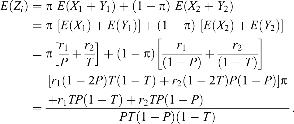
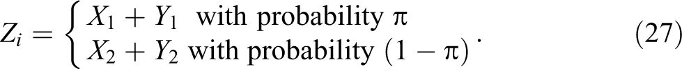
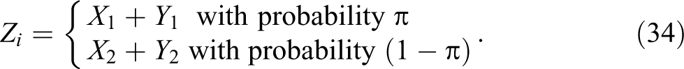
Again let π be the true proportion of the sensitive characteristic in the population who belongs to the group A and $(1 - π)$ be the true proportion of the sensitive characteristic in the population who belong to the nonsensitive group A^c . The distribution of observed responses Z_i , $i = 1, 2, ..., n$ from the n respondents in a sample is then given by:

Z_{i} = {\begin{cases} X_{1} + Y_{1} with probability π \\ X_{2} + Y_{2} with probability (1 - π) \end{cases} .

In other words, the observed response Z_i takes a values of X ₁ + Y ₁ with a probability of π and takes a value of X ₂ + Y ₂ with a probability of (1 − π)

Now, we have the following theorems:

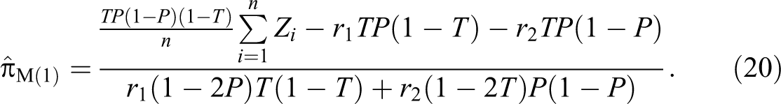
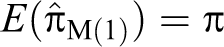
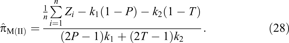
Theorem 1. An unbiased estimator of the population proportion π is given by:

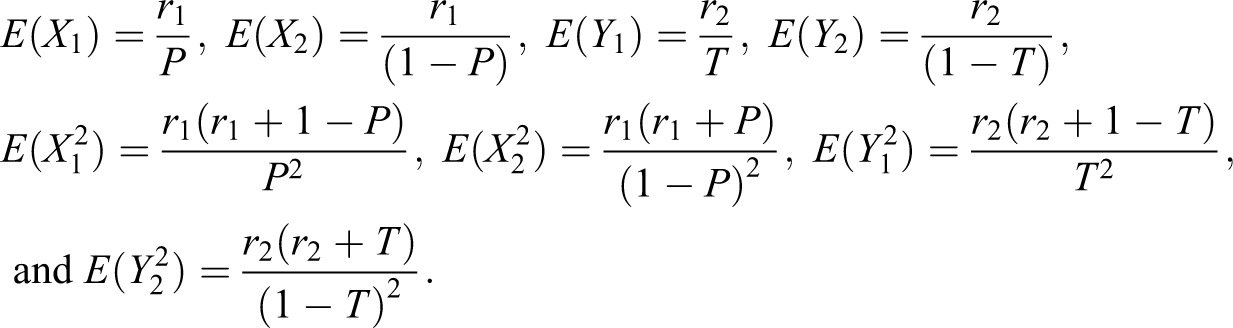
{\hat{π}}_{M(1)} = \frac{\frac{T P (1 - P) (1 - T)}{n} \sum_{i = 1}^{n} Z_{i} - r_{1} T P (1 - T) - r_{2} T P (1 - P)}{r_{1} (1 - 2 P) T (1 - T) + r_{2} (1 - 2 T) P (1 - P)} .

Proof. Given that

X_{1} \sim NB (r_{1}, P)

X_{2} \sim NB (r_{1}, (1 - P))

Y_{1} \sim NB (r_{2}, T)

, and

Y_{2} \sim NB (r_{2}, (1 - T))

, so we have:

E (X_{1}) = \frac{r_{1}}{P}, E (X_{2}) = \frac{r_{1}}{(1 - P)}, E (Y_{1}) = \frac{r_{2}}{T}, and E (Y_{2}) = \frac{r_{2}}{(1 - T)} .

Now by the definition of expected value, from equation (19), we have

E (Z_{i}) = π E (X_{1} + Y_{1}) + (1 - π) E (X_{2} + Y_{2}) = π [E (X_{1}) + E (Y_{1})] + (1 - π) [E (X_{2}) + E (Y_{2})] = π [\frac{r_{1}}{P} + \frac{r_{2}}{T}] + (1 - π) [\frac{r_{1}}{(1 - P)} + \frac{r_{2}}{(1 - T)}] = \frac{\begin{array}{l} [r_{1} (1 - 2 P) T (1 - T) + r_{2} (1 - 2 T) P (1 - P)] π \\ + r_{1} T P (1 - T) + r_{2} T P (1 - P) \end{array}}{P T (1 - P) (1 - T)} .

On solving it for π we have

π = \frac{[P T (1 - P) (1 - T)] E (Z_{i}) - r_{1} T P (1 - T) - r_{2} T P (1 - P)}{[r_{1} (1 - 2 P) T (1 - T) + r_{2} (1 - 2 T) P (1 - P)]} .

By the method of moments, we have the theorem.

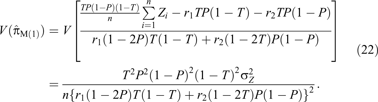
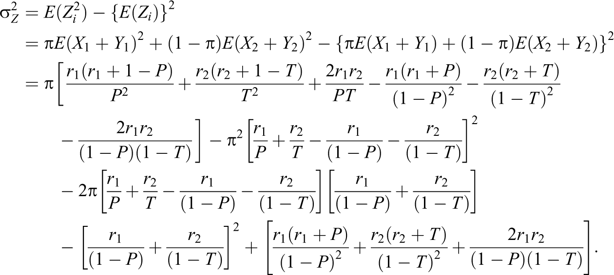
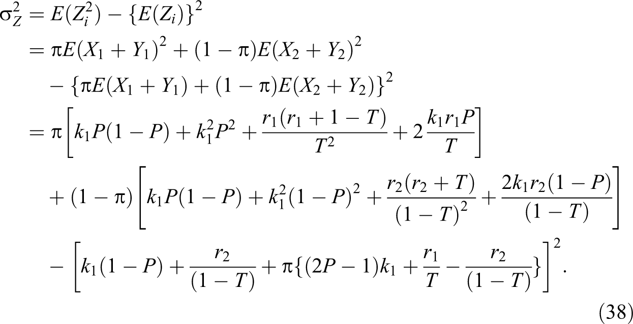
Theorem 2. The variance of the unbiased estimator ${\hat{π}}_{M(1)}$ of the population proportion π is given by:

V ({\hat{π}}_{M(1)}) = \frac{π (1 - π)}{n} + \frac{π [r_{1} T^{2} {(1 - T)}^{2} (1 - 2 P) (1 - P + P^{2}) + r_{2} P^{2} {(1 - P)}^{2} (1 - 2 T) (1 - T + T^{2})]}{n {r_{1} (1 - 2 P) T (1 - T) + r_{2} (1 - 2 T) P (1 - P)}^{2}} + \frac{[r_{1} P^{3} T^{2} {(1 - T)}^{2} + r_{2} P^{2} T^{3} {(1 - P)}^{2}]}{n {r_{1} (1 - 2 P) T (1 - T) + r_{2} (1 - 2 T) P (1 - P)}^{2}} .

Proof. Given that $X_{1} \sim NB (r_{1}, P)$ , $X_{2} \sim NB (r_{1}, (1 - P))$ , $Y_{1} \sim NB (r_{2}, T)$ , and $Y_{2} \sim NB (r_{2}, (1 - T))$ , so we have:

E (X_{1}) = \frac{r_{1}}{P}, E (X_{2}) = \frac{r_{1}}{(1 - P)}, E (Y_{1}) = \frac{r_{2}}{T}, E (Y_{2}) = \frac{r_{2}}{(1 - T)}, E (X_{1}^{2}) = \frac{r_{1} (r_{1} + 1 - P)}{P^{2}}, E (X_{2}^{2}) = \frac{r_{1} (r_{1} + P)}{{(1 - P)}^{2}}, E (Y_{1}^{2}) = \frac{r_{2} (r_{2} + 1 - T)}{T^{2}}, and E (Y_{2}^{2}) = \frac{r_{2} (r_{2} + T)}{{(1 - T)}^{2}} .

Note that all the responses are independent, so by the definition of variance, we have

V ({\hat{π}}_{M(1)}) = V [\frac{\frac{T P (1 - P) (1 - T)}{n} \sum_{i = 1}^{n} Z_{i} - r_{1} T P (1 - T) - r_{2} T P (1 - P)}{r_{1} (1 - 2 P) T (1 - T) + r_{2} (1 - 2 T) P (1 - P)}] = \frac{T^{2} P^{2} {(1 - P)}^{2} {(1 - T)}^{2} σ_{Z}^{2}}{n {r_{1} (1 - 2 P) T (1 - T) + r_{2} (1 - 2 T) P (1 - P)}^{2}} .

where

σ_{Z}^{2} = E (Z_{i}^{2}) - {E (Z_{i})}^{2} = π E {(X_{1} + Y_{1})}^{2} + (1 - π) E {(X_{2} + Y_{2})}^{2} - {π E (X_{1} + Y_{1}) + (1 - π) E (X_{2} + Y_{2})}^{2} = π [\frac{r_{1} (r_{1} + 1 - P)}{P^{2}} + \frac{r_{2} (r_{2} + 1 - T)}{T^{2}} + \frac{2 r_{1} r_{2}}{P T} - \frac{r_{1} (r_{1} + P)}{{(1 - P)}^{2}} - \frac{r_{2} (r_{2} + T)}{{(1 - T)}^{2}} - \frac{2 r_{1} r_{2}}{(1 - P) (1 - T)}] - π^{2} {[\frac{r_{1}}{P} + \frac{r_{2}}{T} - \frac{r_{1}}{(1 - P)} - \frac{r_{2}}{(1 - T)}]}^{2} - 2 π [\frac{r_{1}}{P} + \frac{r_{2}}{T} - \frac{r_{1}}{(1 - P)} - \frac{r_{2}}{(1 - T)}] [\frac{r_{1}}{(1 - P)} + \frac{r_{2}}{(1 - T)}] - {[\frac{r_{1}}{(1 - P)} + \frac{r_{2}}{(1 - T)}]}^{2} + [\frac{r_{1} (r_{1} + P)}{{(1 - P)}^{2}} + \frac{r_{2} (r_{2} + T)}{{(1 - T)}^{2}} + \frac{2 r_{1} r_{2}}{(1 - P) (1 - T)}] .

Now note that we can write:

T^{2} P^{2} {(1 - P)}^{2} {(1 - T)}^{2} σ_{z}^{2} = π (1 - π) {[r_{1} (1 - 2 P) T (1 - T) + r_{2} (1 - 2 T) P (1 - P)]}^{2} + π [r_{1} T^{2} {(1 - T)}^{2} ({(1 - P)}^{3} - P^{3}) + r_{2} P^{2} {(1 - P)}^{2} ({(1 - T)}^{3} - T^{3})] + r_{1} P^{3} T^{2} {(1 - P)}^{2} + r_{2} T^{3} P^{2} {(1 - T)}^{2} .

On using equation (23) in (22), we have the theorem.

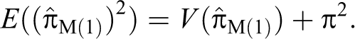
Theorem 3. An unbiased estimator of the variance $V ({\hat{π}}_{M (1)})$ of proposed estimator ${\hat{π}}_{M (1)}$ of the population proportion π is given by:

\hat{V} ({\hat{π}}_{M(1)}) = \frac{{\hat{π}}_{M(1)} (1 - {\hat{π}}_{M(1)})}{n - 1} + \frac{{\hat{π}}_{M(1)} [r_{1} T^{2} {(1 - T)}^{2} (1 - 2 P) (1 - P + P^{2}) + r_{2} P^{2} {(1 - P)}^{2} (1 - 2 T) (1 - T + T^{2})]}{n {r_{1} (1 - 2 P) T (1 - T) + r_{2} (1 - 2 T) P (1 - P)}^{2}} + \frac{[r_{1} P^{3} T^{2} {(1 - T)}^{2} + r_{2} P^{2} T^{3} {(1 - P)}^{2}]}{n {r_{1} (1 - 2 P) T (1 - T) + r_{2} (1 - 2 T) P (1 - P)}^{2}} .

Proof. Note that

E ({\hat{π}}_{M (1)}) = π

and

E ({({\hat{π}}_{M (1)})}^{2}) = V ({\hat{π}}_{M (1)}) + π^{2} .

So we get

E [\frac{{\hat{π}}_{M(1)} (1 - {\hat{π}}_{M(1)})}{n - 1}] = \frac{E ({\hat{π}}_{M(1)}) - E ({({\hat{π}}_{M(1)})}^{2})}{n - 1} = \frac{π (1 - π) - V ({\hat{π}}_{M(1)})}{n - 1} .

Thus, we have the theorem.

Odumade and Singh (2009) have already shown that their proposed model is more efficient than the Warner (1965), Kuk (1990), and Mangat (1994) models for a practicable choice of randomization device parameters. Also Singh and Grewal (2013) have shown that their proposed model can perform better than Kuk (1990) model for certain choices of randomization device parameters. In the Relative Efficiency of the Model I subsection, along similar lines by means of a small-scale simulation study, we investigate situations where the proposed new alternative randomized response model can perform better than the Odumade and Singh (2009) and the Singh and Grewal (2013) models.

Relative Efficiency of the Model I

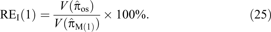
We define the percent relative efficiency of the proposed alternative estimator ${\hat{π}}_{M(1)}$ with respect to the Odumade and Singh (2009) estimator as:

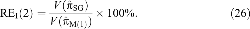
{RE}_{I} (1) = \frac{V ({\hat{π}}_{os})}{V ({\hat{π}}_{M(1)})} \times 100 % .

We also define the percent relative efficiency of the proposed alternative estimator ${\hat{π}}_{M(1)}$ with respect to the Singh and Grewal (2013) estimator as:

{RE}_{I} (2) = \frac{V ({\hat{π}}_{SG})}{V ({\hat{π}}_{M(1)})} \times 100 % .

Note that the RE_I(1) and RE_I(2) values in equations (25) and (26) are free from the sample size but do depend on the choice of randomization device parameters such as P, T, $θ_{1}^{*}$ , $θ_{2}^{*}$ , r ₁, r ₂, and the value of π. We keep the same choice of P and T in the proposed alternative randomized response model and in the Odumade and Singh (2009) model. In this simulation study, we consider four choices of P and T (0.30, 0.35, 0.65, and 0.70) in the proposed and in the Odumade and Singh (2009) models. We set $θ_{1}^{*} = P$ and $θ_{2}^{*} = (1 - P)$ in the Singh and Grewal (2013) model. In addition, we vary the values of r ₁ and r ₂ as 1, 2, and 3. The values of π are changed between 0.1 and 0.9 with a step of 0.1.

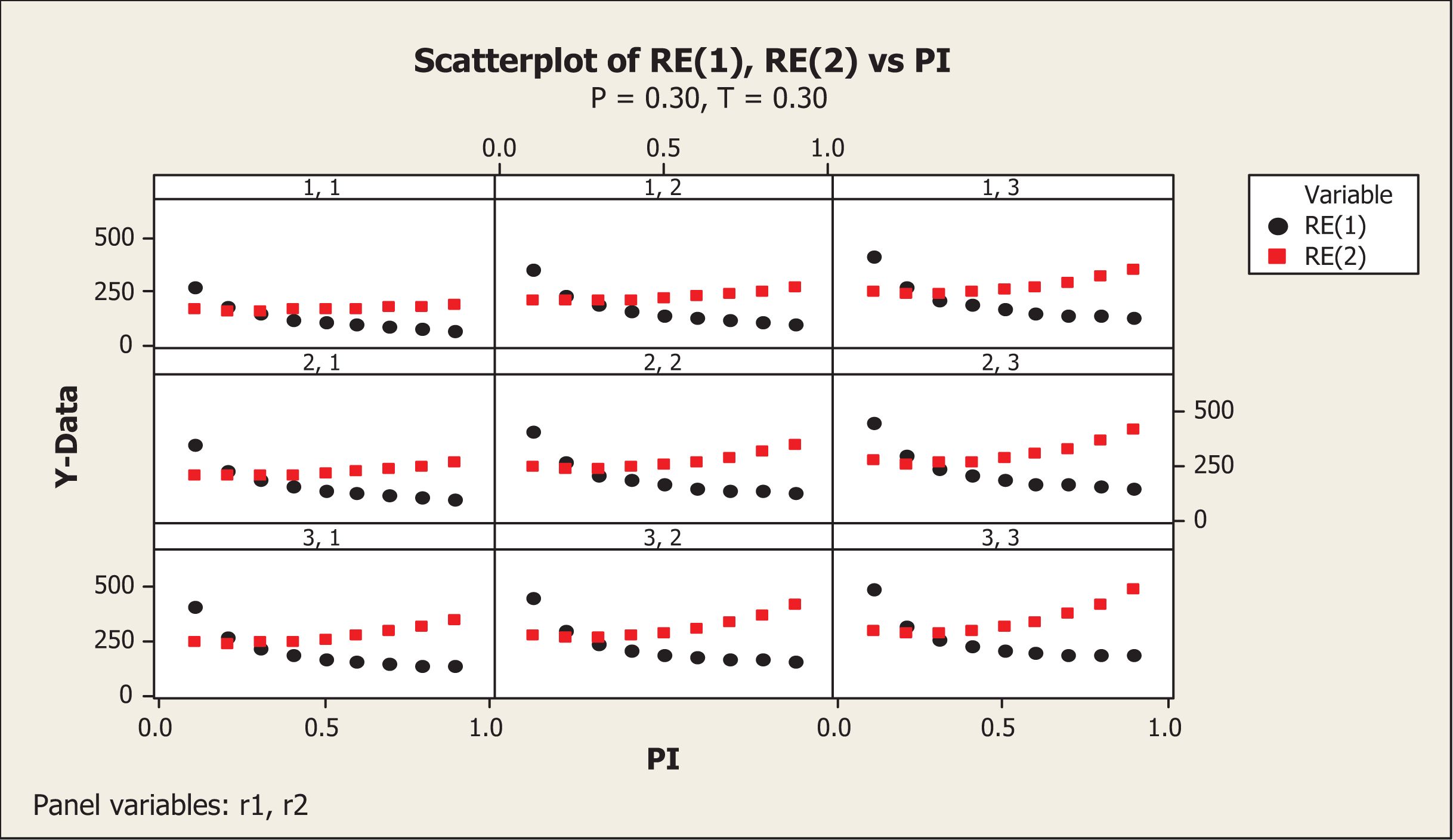
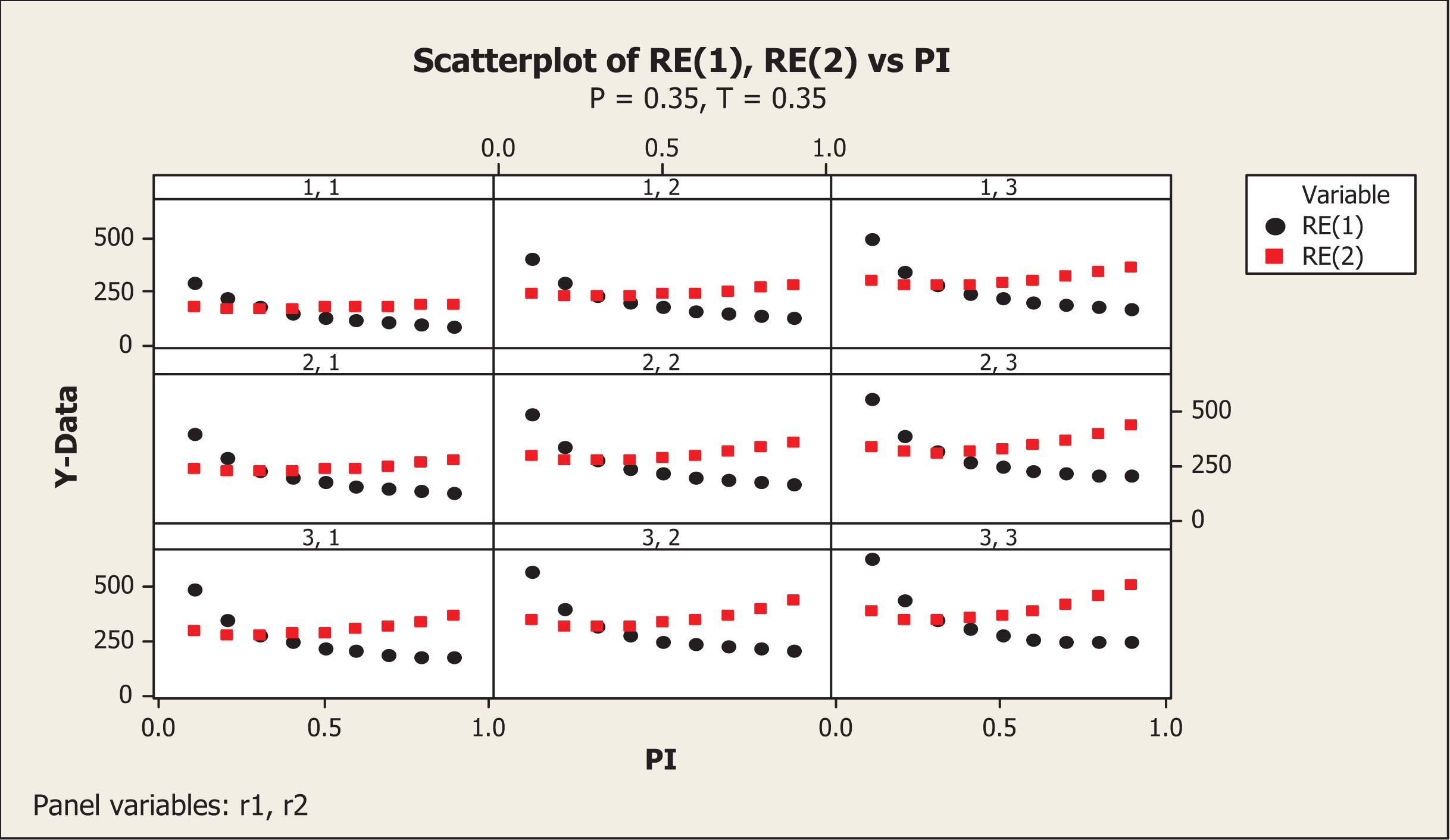
We wrote the FORTRAN codes PRGM1.F95 (see Online Appendix A) to investigate the various situations. In FORTRAN codes, note that $θ_{1}^{*} = P_{1} = P$ and $θ_{2}^{*} = P_{2} = (1 - P)$ . The results obtained by executing the above FORTRAN codes are presented in Table A1 in Online Appendix A. A pictorial presentation of the results given in Table A1 (see Online Appendix A) for P = T = 0.3 and P = T = 0.35 are, respectively, displayed in Figures 2 and 3.

Figure 2.

${RE}_{I} (1)$ and ${RE}_{I} (2)$ values for P = 0.30 and T = 0.30 for different values of $π$ .

Figure 3.

${RE}_{I} (1)$ and ${RE}_{I} (2)$ values for P = 0.35 and T = 0.35 for different values of π.

For P = 0.3 and T = 0.3, if r ₁ = r ₂ = 1 the value of RE_I(1) reaches a maximum of 273.2 percent at π = 0.1, remains higher than 100 percent up to $π = 0.5$ and then reduces to a minimum of 70.2 percent at π = 0.9. Thus, if the value of π is likely to be close to zero, then the choice of P = 0.3 and T = 0.3 for r ₁ =r ₂ = 1 is preferred over the use of the Odumade and Singh (2009) model. The value of RE_I(2) attains 167.1 percent at π = 0.1, 169.8 percent at π = 0.5, and 191.5 percent at π = 0.9. In other words, the proposed new alternative estimator remains more efficient than the Singh and Grewal (2013) model with $θ_{1}^{*} = P = 0.3$ and $θ_{2}^{*} = (1 - P) = 0.7$ for these choices of parameters in the proposed model. For P = 0.3 and T = 0.3, r ₁ = 1 and r ₂ = 2, the RE_I(1) attains 351.9 percent for π = 0.1, reduces to a minimum value of 101.0 percent at π = 0.9, with a median value of 142.6 percent at π = 0.5. The corresponding values of RE_I(2) are 215.1 percent, 275.6 percent, and 221.3 percent, respectively. In other words, the proposed model remains more efficient than the both Odumade and Singh (2009) and Singh and Grewal (2013) models under such circumstances. The same results are observed by interchanging r ₁ = 2 and r ₂ = 1. If r ₁ = 1 and r ₂ = 3, the RE_I(1) and RE_I(2) values become 411.0 percent and 251.3 percent for π = 0.1, 168.1 percent and 260.9 percent for π = 0.5, and 129.4 percent and 353.2 percent for π = 0.9. The same results remain by interchanging the values of r ₁ and r ₂ when keeping the other parameters the same. If r ₁ = 2 and r ₂ = 2, the values of RE_I(1) and RE_I(2) are 411.0 percent and 251.3 percent at π = 0.1, 168.1 percent and 260.9 percent at π = 0.5, and 129.4 percent and 353.2 percent, respectively. If r ₁ = 3 and r ₂ = 3, the values of RE_I(1) and RE_I(2) are 494.1 percent and 302.1 percent at π = 0.1, 204.7 percent and 317.7 percent at π = 0.5, and 180.1 percent and 491.4 percent, respectively. The mirror image of these results, around the value of π = 0.5, is obtained by setting P = 0.7 and T = 0.7. Thus, if π is close to 0, then it is suggested that P and T be chosen less than 0.5 for the proposed model to remain more efficient than the Odumade and Singh (2009) model, while if π is close to 1, it is suggested that P and T be chosen greater than 0.5. The proposed model remains more efficient than the Singh and Grewal (2013) model for all the choices of the parameters considered.

Further note carefully that in the Odumade and Singh (2009) model, each respondent is asked to report a pair of responses as (yes, yes), (yes, no), (no, yes), or (no, no), while in the proposed model a respondent is requested to report only one quantitative response Z_i which is the sum of two numbers resulting from two decks of cards. More cooperation is expected, from a respondent asked to report a single result rather than two results.

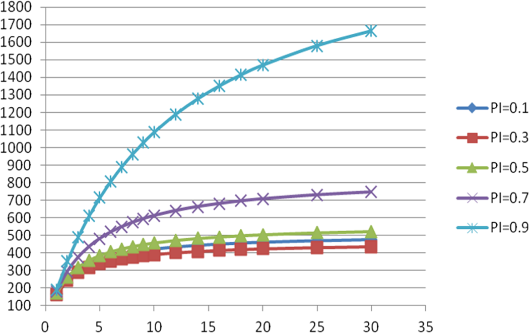
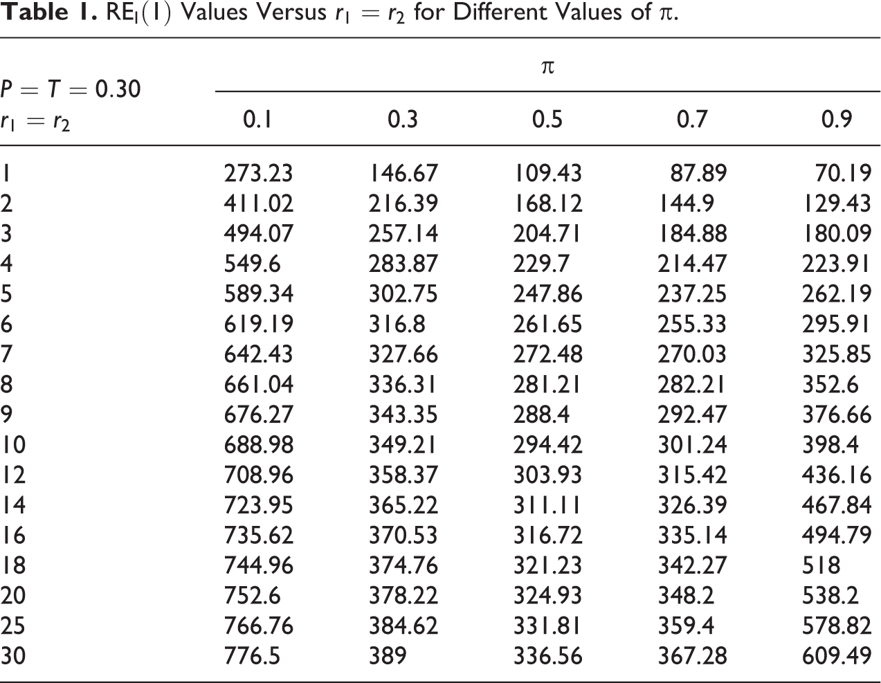
It seems that as the values of r ₁ and r ₂ increase, the RE_I(1) value will go on increasing. From Table 1 and Figure 4 (or Table 2 and Figure 5), it is interesting to note that the value of RE_I(1) increases sharply at the beginning, but later on it becomes almost constant. Thus, higher values of r ₁ and r ₂ may reduce respondents cooperation while increasing the percent relative efficiency RE_I(1) (or RE_I(2)) values only marginally. We wrote the FORTRAN codes PRGM2.F95 (see Online Appendix A) to look for the change in values of RE_I(1) and RE_I(2) while simultaneously increasing the values of r ₁ and r ₂ between 1 and 30 for different values of π between 0.1 and 0.9 with a step of 0.2, for P = T = 0.30. The values of RE_I(1) so obtained are presented in Table 1.

Figure 4.

${RE}_{I} (1)$ versus $r_{1} = r_{2}$ for different values of π = 0.1, 0.3, 0.5, 0.7, and 0.9.

Figure 5.

${RE}_{I} (2)$ versus $r_{1} = r_{2}$ for different values of π = 0.1, 0.3, 0.5, 0.7, and 0.9.

Table 1.

${RE}_{I} (1)$ Values Versus $r_{1} = r_{2}$ for Different Values of π.

$P = T = 0.30$	π
$r_{1} = r_{2}$	0.1	0.3	0.5	0.7	0.9
1	273.23	146.67	109.43	87.89	70.19
2	411.02	216.39	168.12	144.9	129.43
3	494.07	257.14	204.71	184.88	180.09
4	549.6	283.87	229.7	214.47	223.91
5	589.34	302.75	247.86	237.25	262.19
6	619.19	316.8	261.65	255.33	295.91
7	642.43	327.66	272.48	270.03	325.85
8	661.04	336.31	281.21	282.21	352.6
9	676.27	343.35	288.4	292.47	376.66
10	688.98	349.21	294.42	301.24	398.4
12	708.96	358.37	303.93	315.42	436.16
14	723.95	365.22	311.11	326.39	467.84
16	735.62	370.53	316.72	335.14	494.79
18	744.96	374.76	321.23	342.27	518
20	752.6	378.22	324.93	348.2	538.2
25	766.76	384.62	331.81	359.4	578.82
30	776.5	389	336.56	367.28	609.49

Table 2.

${RE}_{I} (2)$ Values $r_{1} = r_{2}$ for Different Values of π.

$P = T = 0.30$	π
$r_{1} = r_{2}$	0.1	0.3	0.5	0.7	0.9
1	167.05	164.44	169.81	178.69	191.53
2	251.29	242.62	260.87	294.62	353.17
3	302.07	288.31	317.65	375.9	491.4
4	336.02	318.28	356.44	436.05	610.97
5	360.32	339.45	384.62	482.37	715.41
6	378.56	355.2	406.02	519.13	807.43
7	392.77	367.38	422.82	549.01	889.12
8	404.15	377.07	436.36	573.79	962.13
9	413.47	384.97	447.51	594.65	1,027.76
10	421.23	391.53	456.85	612.48	1,087.09
12	433.45	401.81	471.62	641.31	1,190.14
14	442.62	409.49	482.76	663.62	1,276.57
16	449.75	415.44	491.47	681.4	1,350.12
18	455.46	420.19	498.46	695.9	1,413.45
20	460.13	424.07	504.2	707.95	1,468.56
25	468.79	431.24	514.87	730.73	1,579.4
30	474.74	436.15	522.24	746.75	1,663.09

A pictorial presentation of results in Table 1 is shown in Figure 4. From Figure 4, it is clear that if the value of $r_{1} = r_{2}$ is more than 10, then the percentage relative gain is not as steep as for a choice of value of r ₁ = r ₂ between 1 and 5 for all possible values of π considered (0.1, 0.3, 0.5, 0.7, and 0.9) and P = T = 0.30.

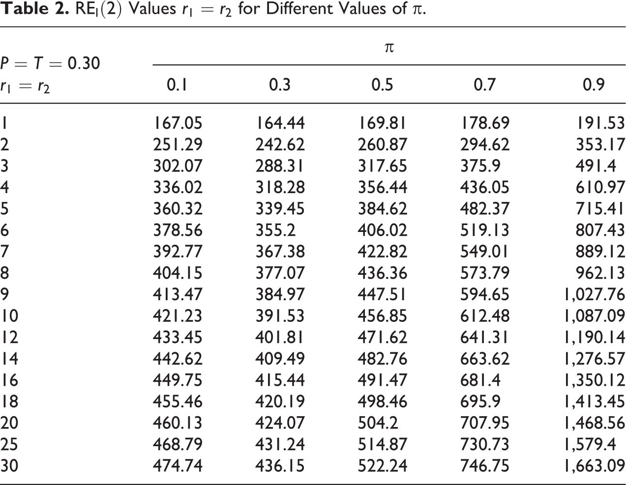
For demonstration purposes, we provide in Table 2 the values of ${RE}_{I} (2)$ as a function of $r_{1} = r_{2}$ for different choice of the proportion of sensitive characteristic π in a population for $P = T = 0.30$ .

A pictorial presentation of results in Table 2 is shown in Figure 5. From Figure 5, it is again clear that if the value of $r_{1} = r_{2}$ is more than 10, then the percentage relative gain is not as steep as for a choice of value of $r_{1} = r_{2}$ between 1 and 5, for all possible values of π considered (0.1, 0.3, 0.5, 0.7, and 0.9). Thus, it seems that increasing the values of $r_{1}$ and $r_{2}$ will only marginally increase the percent relative efficiency of the proposed estimator.

In the next section, we consider a further extension of the Odumade and Singh (2009) technique based on multiple trials per respondent which leads to a new alternative randomized response model, say model II.

Model II

Using the same decks of cards as before, respondents are asked to draw cards at random with replacement from each of the decks and, based on whether they belong to group A or not, to report different things.

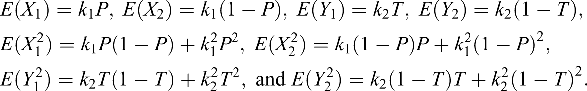
Case I: Respondent belongs to group A. In this case, the respondent is to draw $k_{1}$ cards from deck I. Let $X_{1}$ be the number of red cards drawn. They are to draw $k_{2}$ cards from deck II. Let $Y_{1}$ be the number of red cards drawn. Clearly, $X_{1}$ and $Y_{1}$ are binomial random variables with $X_{1} \sim B (k_{1}, P)$ and $Y_{1} \sim B (k_{2}, T)$ . Finally, they are to report the sum $(X_{1} + Y_{1})$ .

Case II: Respondent does not belong to group A. In this case, the respondent is asked to draw $k_{1}$ cards from deck I. Let $X_{2}$ be the number of green cards drawn. They are to draw $k_{2}$ cards from deck II. Let $Y_{2}$ be the number of green cards drawn. Again $X_{2}$ and $Y_{2}$ are binomial random variables with $X_{2} \sim B (k_{1}, (1 - P))$ and $Y_{2} \sim B (k_{2}, (1 - T))$ . Finally, they are to report the sum $(X_{2} + Y_{2})$ .

Let $π$ be the true proportion of the sensitive characteristic in the population who belongs to the group A and $(1 - π)$ be the true proportion of the sensitive characteristic in the population who belong to the nonsensitive group A^c . The distribution of observed responses Z_i , $i = 1, 2, ..., n$ from the n respondents in a sample is then given by:

Z_{i} = {\begin{cases} X_{1} + Y_{1} with probability π \\ X_{2} + Y_{2} with probability (1 - π) \end{cases} .

In other words, the observed response $Z_{i}$ takes a values of $X_{1} + Y_{1}$ with a probability of π and takes a value of $X_{2} + Y_{2}$ with a probability of $(1 - π) .$

Now, we have the following theorems.

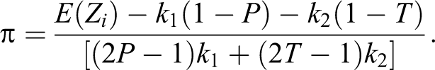
Theorem 4. An unbiased estimator ${\hat{π}}_{M(II)}$ of the population proportion π is given by:

{\hat{π}}_{M(II)} = \frac{\frac{1}{n} \sum_{i = 1}^{n} Z_{i} - k_{1} (1 - P) - k_{2} (1 - T)}{(2 P - 1) k_{1} + (2 T - 1) k_{2}} .

Proof. Given that $X_{1} \sim B (k_{1}, P)$ , $X_{2} \sim B (k_{1}, (1 - P))$ , $Y_{1} \sim B (k_{2}, T)$ , and $Y_{2} \sim B (k_{2}, (1 - T))$ , so we have:

E (X_{1}) = k_{1} P, E (X_{2}) = k_{1} (1 - P), E (Y_{1}) = k_{2} T, and E (Y_{2}) = k_{2} (1 - T),

Now by the definition of expected value, from (27), we have

E (Z_{i}) = π E (X_{1} + Y_{1}) + (1 - π) E (X_{2} + Y_{2}) = π [E (X_{1}) + E (Y_{1})] + (1 - π) [E (X_{2}) + E (Y_{2})] = π [k_{1} P + k_{2} T] + (1 - π) [k_{1} (1 - P) + k_{2} (1 - T)] = π [(2 P - 1) k_{1} + (2 T - 1) k_{2}] + k_{1} (1 - P) + k_{2} (1 - T) .

On solving it for π, we have

π = \frac{E (Z_{i}) - k_{1} (1 - P) - k_{2} (1 - T)}{[(2 P - 1) k_{1} + (2 T - 1) k_{2}]} .

By the method of moments, we have the theorem.

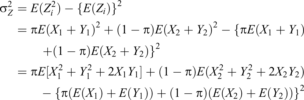
Theorem 5. The variance of the unbiased estimator ${\hat{π}}_{M(II)}$ of the population proportion π is given by:

V ({\hat{π}}_{M(II)}) = \frac{π (1 - π)}{n} + \frac{k_{1} P (1 - P) + k_{2} T (1 - T)}{n {[(2 P - 1) k_{1} + (2 T - 1) k_{2}]}^{2}} .

Proof. Given $X_{1} \sim B (k_{1}, P)$ , $X_{2} \sim B (k_{1}, (1 - P))$ , $Y_{1} \sim B (k_{2}, T)$ , and $Y_{2} \sim B (k_{2}, (1 - T))$ ,

so we have:

E (X_{1}) = k_{1} P, E (X_{2}) = k_{1} (1 - P), E (Y_{1}) = k_{2} T, E (Y_{2}) = k_{2} (1 - T), E (X_{1}^{2}) = k_{1} P (1 - P) + k_{1}^{2} P^{2}, E (X_{2}^{2}) = k_{1} (1 - P) P + k_{1}^{2} {(1 - P)}^{2}, E (Y_{1}^{2}) = k_{2} T (1 - T) + k_{2}^{2} T^{2}, and E (Y_{2}^{2}) = k_{2} (1 - T) T + k_{2}^{2} {(1 - T)}^{2} .

Note that all the responses are independent, so by the definition of variance, we have

V ({\hat{π}}_{M(II)}) = V [\frac{\frac{1}{n} \sum_{i = 1}^{n} Z_{i} - k_{1} (1 - P) - k_{2} (1 - T)}{(2 P - 1) k_{1} + (2 T - 1) k_{2}}] = \frac{\frac{1}{n^{2}} \sum_{i = 1}^{n} V (Z_{i})}{{(2 P - 1) k_{1} + (2 T - 1) k_{2}}^{2}} = \frac{σ_{Z}^{2}}{n {(2 P - 1) k_{1} + (2 T - 1) k_{2}}^{2}},

where

σ_{Z}^{2} = E (Z_{i}^{2}) - {E (Z_{i})}^{2} = π E {(X_{1} + Y_{1})}^{2} + (1 - π) E {(X_{2} + Y_{2})}^{2} - {π E (X_{1} + Y_{1}) + (1 - π) E (X_{2} + Y_{2})}^{2} = π E [X_{1}^{2} + Y_{1}^{2} + 2 X_{1} Y_{1}] + (1 - π) E (X_{2}^{2} + Y_{2}^{2} + 2 X_{2} Y_{2}) - {π (E (X_{1}) + E (Y_{1})) + (1 - π) (E (X_{2}) + E (Y_{2}))}^{2}

= π [E (X_{1}^{2}) + E (Y_{1}^{2}) + 2 E (X_{1}) E (Y_{1})] + (1 - π) (E (X_{2}^{2}) + E (Y_{2}^{2}) + 2 E (X_{2}) E (Y_{2})) - {π (E (X_{1}) + E (Y_{1})) + (1 - π) (E (X_{2}) + E (Y_{2}))}^{2}

= π [k_{1} P (1 - P) + k_{2} T (1 - T) + {(k_{1} P + k_{2} T)}^{2}] + (1 - π) [k_{1} P (1 - P) + k_{2} T (1 - T) + {(k_{1} (1 - P) + k_{2} (1 - T))}^{2}] - {[π {2 (k_{1} P + k_{2} T) - k_{1} - k_{2}} + k_{1} (1 - P) + k_{2} (1 - T)]}^{2}

= k_{1} P (1 - P) + k_{2} T (1 - T) - π^{2} {[(2 P - 1) k_{1} + (2 T - 1) k_{2}]}^{2} + π {[(2 P - 1) k_{1} + (2 T - 1) k_{2}]}^{2} .

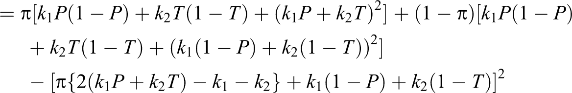
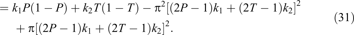
We have (31) because:

k_{1} P (1 - P) + k_{2} T (1 - T) + {(k_{1} P + k_{2} T)}^{2} - k_{1} P (1 - P) - k_{2} T (1 - T) - {k_{1} (1 - P) + k_{2} (1 - T)}^{2} - 2 {(2 P - 1) k_{1} + (2 T - 1) k_{2}} (k_{1} (1 - P) + k_{2} (1 - T)} - {(2 P - 1) k_{1} + (2 T - 1) k_{2}}^{2} = 0.

On using (31) in (30), we have the theorem.

Theorem 6. An unbiased estimator of the variance $V ({\hat{π}}_{M(II)})$ of the proposed estimator ${\hat{π}}_{M(II)}$ of the population proportion π is given by:

\hat{V} ({\hat{π}}_{M(II)}) = \frac{{\hat{π}}_{M(II)} (1 - {\hat{π}}_{M(II)})}{n - 1} + \frac{k_{1} P (1 - P) + k_{2} T (1 - T)}{n {(2 P - 1) k_{1} + (2 T - 1) k_{2}}^{2}} .

Proof. Note that

E ({\hat{π}}_{M(II)}) = π

and

E ({({\hat{π}}_{M(II)})}^{2}) = V ({\hat{π}}_{M(II)}) + π^{2} .

So we get

E [\frac{{\hat{π}}_{M(II)} (1 - {\hat{π}}_{M(II)})}{n - 1}] = \frac{E ({\hat{π}}_{M(II)}) - E ({({\hat{π}}_{M(II)})}^{2})}{n - 1} = \frac{π - (V ({\hat{π}}_{M(II)}) + π^{2})}{n - 1}

= \frac{π (1 - π) - V ({\hat{π}}_{M(II)})}{n - 1},

which proves the theorem.

In the Relative Efficiency of the Model II subsection, we investigate situations where the proposed fixed multiple trial randomized response model (model II) can perform better than the Odumade and Singh (2009) model.

Relative Efficiency of the Model II

We define the percent relative efficiency of the proposed multi trial alternative estimator ${\hat{π}}_{M(II)}$ with respect to the Odumade and Singh (2009) estimator as:

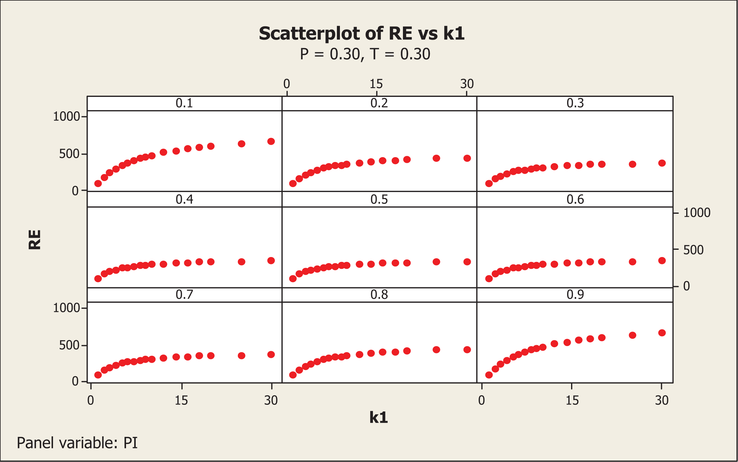
{RE}_{II} (1) = \frac{V ({\hat{π}}_{os})}{V ({\hat{π}}_{M(II)})} \times 100 % .

Note that the ${RE}_{II} (1)$ values are free from the sample size but depend on the choice of randomization device parameters such as P, T, k ₁, k ₂, and the value of π. We keep the same choice of P, and T in the proposed multiple trial alternative randomized response model (model II) as in the Odumade and Singh (2009) model. In this simulation study, we consider four choices of P and T as 0.30, 0.35, 0.65, and 0.70 in the proposed multiple trial and the Odumade and Singh (2009) models. We varied the values of k ₁ and k ₂ from 1 to 30 to investigate whether the increase in the number of trials per respondent increases the efficiency of the estimator. We kept k ₁ equal to k ₂; in addition, the values of π were varied between 0.1 and 0.9 with a stepping of 0.1. We wrote the FORTRAN codes PRGM3.F95 (see Online Appendix A) to investigate the different situations. Executing the FORTRAN codes lead to the results listed in Table A.2, as given in Online Appendix A.

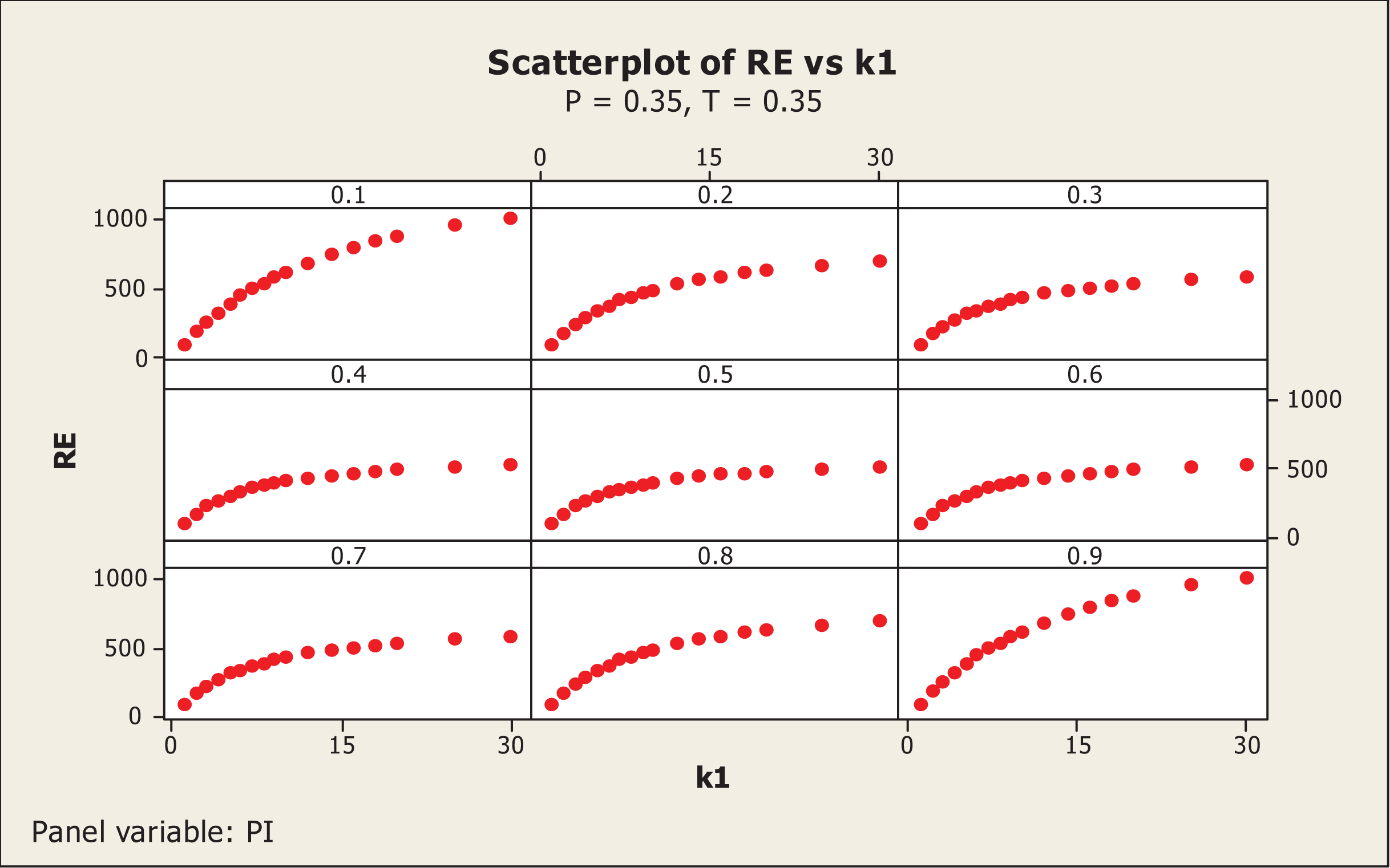
From the results in Table A2, it is clear that the values of ${RE}_{II} (1)$ are equal for $(P, T) = (0.30, 0.30)$ and $(P, T) = (0.70, 0.70)$ and are again equal for $(P, T) = (0.35, 0.35)$ and $(P, T) = (0.65, 0.65)$ . To look at the behavior of the relative efficiency, ${RE}_{II} (1)$ values as k ₁ and k ₂ increase, we plotted ${RE}_{II} (1)$ versus $k_{1} (= k_{2})$ for each value of π. This was done for each of the chosen values of $P (= T)$ and is presented in Figures 6 and 7. The results for the choice of $(P, T) = (0.70, 0.70)$ are mirror image of the results for $(P, T) = (0.30, 0.30)$ , and the results for $(P, T) = (0.65, 0.65)$ are mirror image of $(P, T) = (0.35, 0.35)$ , so those results are not presented in separate figures than Figures 6 and 7. From the graphical presentations, it is clear that just increasing the number of cards a respondent is to draw increases efficiency, but only to a certain point after which any increase is minimal. Note that if $k_{1} = k_{2} = 1$ , then the proposed estimator has efficiency of 100 percent (if P = T). In another study, we found that if $P \neq T$ , then the proposed estimator may perform worse than the Odumade and Singh (2009) model for $k_{1} = k_{2} = 1$ irrespective of the value of π. Thus, based on our study, we suggest using $k_{1} = k_{2}$ with a value between 2 and 6 which should not affect respondents’ cooperation. Requiring too many trials per respondent may at times be unacceptable; however, in the proposed model only a single response (the sum) is requested, so it seems likely that we would not be risking a loss of cooperation.

Figure 6.

The ${RE}_{II} (1)$ versus $k_{1} (= k_{2})$ with P = 0.30 and T = 0.30 for $π \in [0.1, 0.9]$ .

Figure 7.

The ${RE}_{II} (1)$ versus $k_{1} (= k_{2})$ with P = 0.35 and T = 0.35 for $π \in [0.1, 0.9]$ .

In the next section, we consider a further extension of the Odumade and Singh (2009) model based on “fixed and targeted trials” per respondent, which leads to a new alternative randomized response model.

Model III

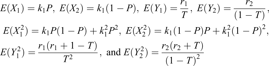
Case I: Respondent belongs to group A. In this case, the respondent is asked to draw k ₁ cards from deck I. Let $X_{1}$ be the number of red cards drawn. They are then to draw cards from deck II until $r_{1}$ red cards appear. Let $Y_{1}$ be the number of cards drawn. In this case, $X_{1} \sim B (k_{1}, P)$ , that is $X_{1}$ follows a binomial distribution with parameters k ₁ and P; and $Y_{1} \sim N B (r_{1}, T)$ that is $Y_{1}$ follows a negative binomial distribution with parameters $r_{1}$ and T. Finally they are to report the sum ( $X_{1} + Y_{1}$ ).

Case II: Respondent does not belong to group A. In this case, the respondent is asked to draw k ₁ cards from deck I. Let $X_{2}$ be the number of green cards drawn. They are to draw cards from deck II. Let $Y_{2}$ be the number of green cards drawn. In this case, $X_{2} \sim B (k_{1}, (1 - P))$ , that is $X_{2}$ follows a binomial distribution with parameters k ₁ and $(1 - P)$ , and $Y_{2} \sim N B (r_{2}, (1 - T))$ that is $Y_{2}$ follows a negative binomial distribution with parameters $r_{2}$ and $(1 - T)$ . Finally, they are to report the sum (X ₂ + Y ₂).

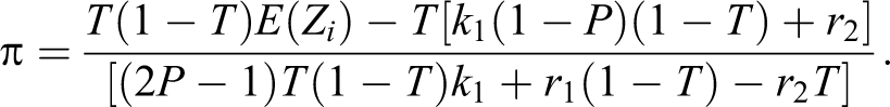
Taking π as before the true proportion of the sensitive characteristic in the population who belongs to the group A and $(1 - π)$ be the true proportion of the sensitive characteristic in the population who belong to the nonsensitive group A^c , the distribution of observed responses $Z_{i}$ , $i = 1, 2, ..., n$ from the n respondents in a sample is again given by:

Z_{i} = {\begin{cases} X_{1} + Y_{1} with probability π \\ X_{2} + Y_{2} with probability (1 - π) \end{cases} .

In other words, the observed response $Z_{i}$ takes a values of $X_{1} + Y_{1}$ with a probability of π and takes a value of $X_{2} + Y_{2}$ with a probability of $(1 - π)$ .

Now, we have the following theorems.

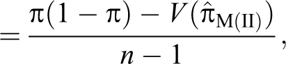
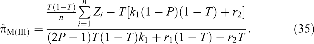
Theorem 7. An unbiased estimator ${\hat{π}}_{M(III)}$ of the population proportion π is given by:

{\hat{π}}_{M(III)} = \frac{\frac{T (1 - T)}{n} \sum_{i = 1}^{n} Z_{i} - T [k_{1} (1 - P) (1 - T) + r_{2}]}{(2 P - 1) T (1 - T) k_{1} + r_{1} (1 - T) - r_{2} T} .

Proof. Given that $X_{1} \sim B (k_{1}, P)$ , $X_{2} \sim B (k_{1}, (1 - P))$ , $Y_{1} \sim NB (r_{1}, T)$ , and $Y_{2} \sim NB (r_{2}, (1 - T))$ , so we have:

E (X_{1}) = k_{1} P, E (X_{2}) = k_{1} (1 - P), E (Y_{1}) = \frac{r_{1}}{T}, and E (Y_{2}) = \frac{r_{2}}{(1 - T)} .

Now by the definition of expected value, from (34), we have

E (Z_{i}) = π E (X_{1} + Y_{1}) + (1 - π) E (X_{2} + Y_{2}) = π [E (X_{1}) + E (Y_{1})] + (1 - π) [E (X_{2}) + E (Y_{2})] = π [k_{1} P + \frac{r_{1}}{T}] + (1 - π) [k_{1} (1 - P) + \frac{r_{2}}{(1 - T)}] .

On solving it for π, we have

π = \frac{T (1 - T) E (Z_{i}) - T [k_{1} (1 - P) (1 - T) + r_{2}]}{[(2 P - 1) T (1 - T) k_{1} + r_{1} (1 - T) - r_{2} T]} .

So we have

E (Z_{i}) = \frac{π [(2 P - 1) T (1 - T) k_{1} + r_{1} (1 - T) - r_{2} T] + T [k_{1} (1 - P) (1 - T) + r_{2}]}{T (1 - T)} .

Taking expected value on both sides of (35), we have

E ({\hat{π}}_{M(III)}) = \frac{\frac{T (1 - T)}{n} \sum_{i = 1}^{n} E (Z_{i}) - T [k_{1} (1 - P) (1 - T) + r_{2}]}{(2 P - 1) T (1 - T) k_{1} + r_{1} (1 - T) - r_{2} T} = π,

which proves the unbiasedness.

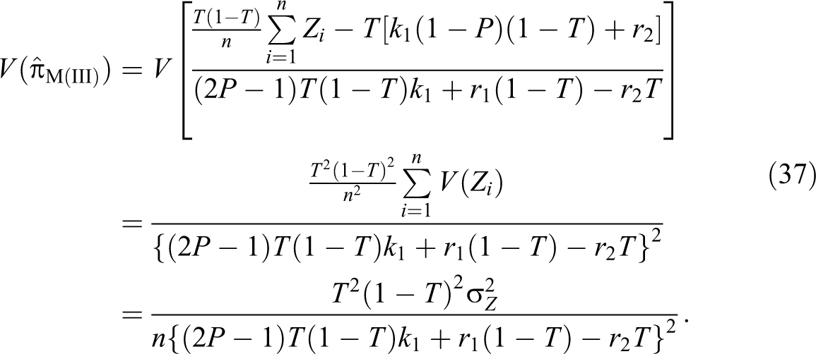
Theorem 8. The variance of the unbiased estimator ${\hat{π}}_{M(III)}$ of the population proportion π is given by:

\begin{array}{l} V ({\hat{π}}_{M(III)}) = \frac{π (1 - π)}{n} + \frac{k_{1}^{2} T^{2} {(1 - T)}^{2} P (1 - P) + T^{3}}{n {[T (1 - T) (2 P - 1) k_{1} + r_{1} (1 - T) - r_{2} T]}^{2}} \\ + \frac{\begin{array}{l} π [r_{1} {(1 - T)}^{3} - r_{2} T^{3} - 2 r_{1} r_{2} T (1 - T) \\ - 2 r_{2} k_{1}^{2} (1 - P) (1 - T) T^{2} - 2 T^{2} (2 P - 1) (1 - p) {(1 - T)}^{2} k_{1}^{2}] \end{array}}{n {[T (1 - T) (2 P - 1) k_{1} + r_{1} (1 - T) - r_{2} T]}^{2}} . \end{array}

Proof. Given $X_{1} \sim B (k_{1}, P)$ , $X_{2} \sim B (k_{1}, (1 - P))$ , $Y_{1} \sim NB (r_{1}, T)$ , and $Y_{2} \sim NB (r_{2}, (1 - T))$ , we have:

E (X_{1}) = k_{1} P, E (X_{2}) = k_{1} (1 - P), E (Y_{1}) = \frac{r_{1}}{T}, E (Y_{2}) = \frac{r_{2}}{(1 - T)}, E (X_{1}^{2}) = k_{1} P (1 - P) + k_{1}^{2} P^{2}, E (X_{2}^{2}) = k_{1} (1 - P) P + k_{1}^{2} {(1 - P)}^{2}, E (Y_{1}^{2}) = \frac{r_{1} (r_{1} + 1 - T)}{T^{2}}, and E (Y_{2}^{2}) = \frac{r_{2} (r_{2} + T)}{{(1 - T)}^{2}}

Note that all the responses are independent, so by the definition of variance, we have

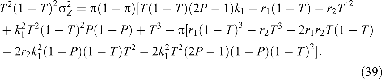
V ({\hat{π}}_{M(III)}) = V [\frac{\frac{T (1 - T)}{n} \sum_{i = 1}^{n} Z_{i} - T [k_{1} (1 - P) (1 - T) + r_{2}]}{(2 P - 1) T (1 - T) k_{1} + r_{1} (1 - T) - r_{2} T}] = \frac{\frac{T^{2} {(1 - T)}^{2}}{n^{2}} \sum_{i = 1}^{n} V (Z_{i})}{{(2 P - 1) T (1 - T) k_{1} + r_{1} (1 - T) - r_{2} T}^{2}} = \frac{T^{2} {(1 - T)}^{2} σ_{Z}^{2}}{n {(2 P - 1) T (1 - T) k_{1} + r_{1} (1 - T) - r_{2} T}^{2}} .

where

σ_{Z}^{2} = E (Z_{i}^{2}) - {E (Z_{i})}^{2} = π E {(X_{1} + Y_{1})}^{2} + (1 - π) E {(X_{2} + Y_{2})}^{2} - {π E (X_{1} + Y_{1}) + (1 - π) E (X_{2} + Y_{2})}^{2} = π [k_{1} P (1 - P) + k_{1}^{2} P^{2} + \frac{r_{1} (r_{1} + 1 - T)}{T^{2}} + 2 \frac{k_{1} r_{1} P}{T}] + (1 - π) [k_{1} P (1 - P) + k_{1}^{2} {(1 - P)}^{2} + \frac{r_{2} (r_{2} + T)}{{(1 - T)}^{2}} + \frac{2 k_{1} r_{2} (1 - P)}{(1 - T)}] - {[k_{1} (1 - P) + \frac{r_{2}}{(1 - T)} + π {(2 P - 1) k_{1} + \frac{r_{1}}{T} - \frac{r_{2}}{(1 - T)}}]}^{2} .

Now using (38), we have

T^{2} {(1 - T)}^{2} σ_{Z}^{2} = π (1 - π) {[T (1 - T) (2 P - 1) k_{1} + r_{1} (1 - T) - r_{2} T]}^{2} + k_{1}^{2} T^{2} {(1 - T)}^{2} P (1 - P) + T^{3} + π [r_{1} {(1 - T)}^{3} - r_{2} T^{3} - 2 r_{1} r_{2} T (1 - T) - 2 r_{2} k_{1}^{2} (1 - P) (1 - T) T^{2} - 2 k_{1}^{2} T^{2} (2 P - 1) (1 - P) {(1 - T)}^{2}] .

On using (39) in (37), we have the theorem.

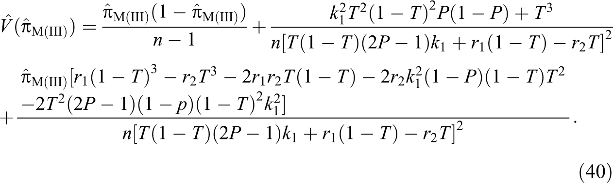
Theorem 9. An unbiased estimator of the variance $V ({\hat{π}}_{M(III)})$ of the proposed estimator ${\hat{π}}_{M(III)}$ of the population proportion π is given by:

\begin{array}{l} \hat{V} ({\hat{π}}_{M(III)}) = \frac{{\hat{π}}_{M (III)} (1 - {\hat{π}}_{M(III)})}{n - 1} + \frac{k_{1}^{2} T^{2} {(1 - T)}^{2} P (1 - P) + T^{3}}{n {[T (1 - T) (2 P - 1) k_{1} + r_{1} (1 - T) - r_{2} T]}^{2}} \\ + \frac{\begin{array}{l} {\hat{π}}_{M(III)} [r_{1} {(1 - T)}^{3} - r_{2} T^{3} - 2 r_{1} r_{2} T (1 - T) - 2 r_{2} k_{1}^{2} (1 - P) (1 - T) T^{2} \\ - 2 T^{2} (2 P - 1) (1 - p) {(1 - T)}^{2} k_{1}^{2}] \end{array}}{n {[T (1 - T) (2 P - 1) k_{1} + r_{1} (1 - T) - r_{2} T]}^{2}} . \end{array}

Proof. Note that

E ({\hat{π}}_{M(III)}) = π and E ({({\hat{π}}_{M(III)})}^{2}) = V ({\hat{π}}_{M(III)}) + π^{2}

So we get

E [\frac{{\hat{π}}_{M(III)} (1 - {\hat{π}}_{M(III)})}{n - 1}] = \frac{E ({\hat{π}}_{M(III)}) - E ({({\hat{π}}_{M(III)})}^{2})}{n - 1} = \frac{π (1 - π) - V ({\hat{π}}_{M(III)})}{n - 1}

which proves the theorem.

In the Relative Efficiency of the Model III subsection, we investigate situations where the proposed fixed and targeted trials randomized response model (model III) can perform better than the Odumade and Singh (2009) model.

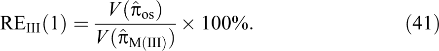
Relative Efficiency of the Model III

We define the percent relative efficiency of the proposed estimator ${\hat{π}}_{M(III)}$ with respect to the Odumade and Singh (2009) estimator as:

{RE}_{III} (1) = \frac{V ({\hat{π}}_{os})}{V ({\hat{π}}_{M(III)})} \times 100 % .

Note that the ${RE}_{III} (1)$ values are free from the sample size but depend on the choice of randomization device parameters such as P, T, $k_{1}$ , $r_{1}$ , $r_{2}$ , and the value of π. We keep the same choice of P, and T in the proposed model III as in the Odumade and Singh (2009) model. In this simulation study, we consider four choices of P and T as 0.30, 0.35, 0.65, and 0.70 in the proposed fixed and targeted model and the Odumade and Singh (2009) model. In addition, we vary the values of $k_{1}$ , $r_{1}$ , and $r_{2}$ as 1, 2, 3 to search those choices for which the percent relative efficiency value remain higher than 100 percent. The values of π are changed between 0.1 and 0.9 with a step of 0.1. We wrote the FORTRAN codes PRGM4.F95 (see Online Appendix A) to investigate the different situations. Executing the above codes lead to the results listed in Table A3 (See Online Appendix A). From these results, one could conclude that the proposed model III can also be used to produce more efficient estimate than the Odumade and Singh (2009) model.

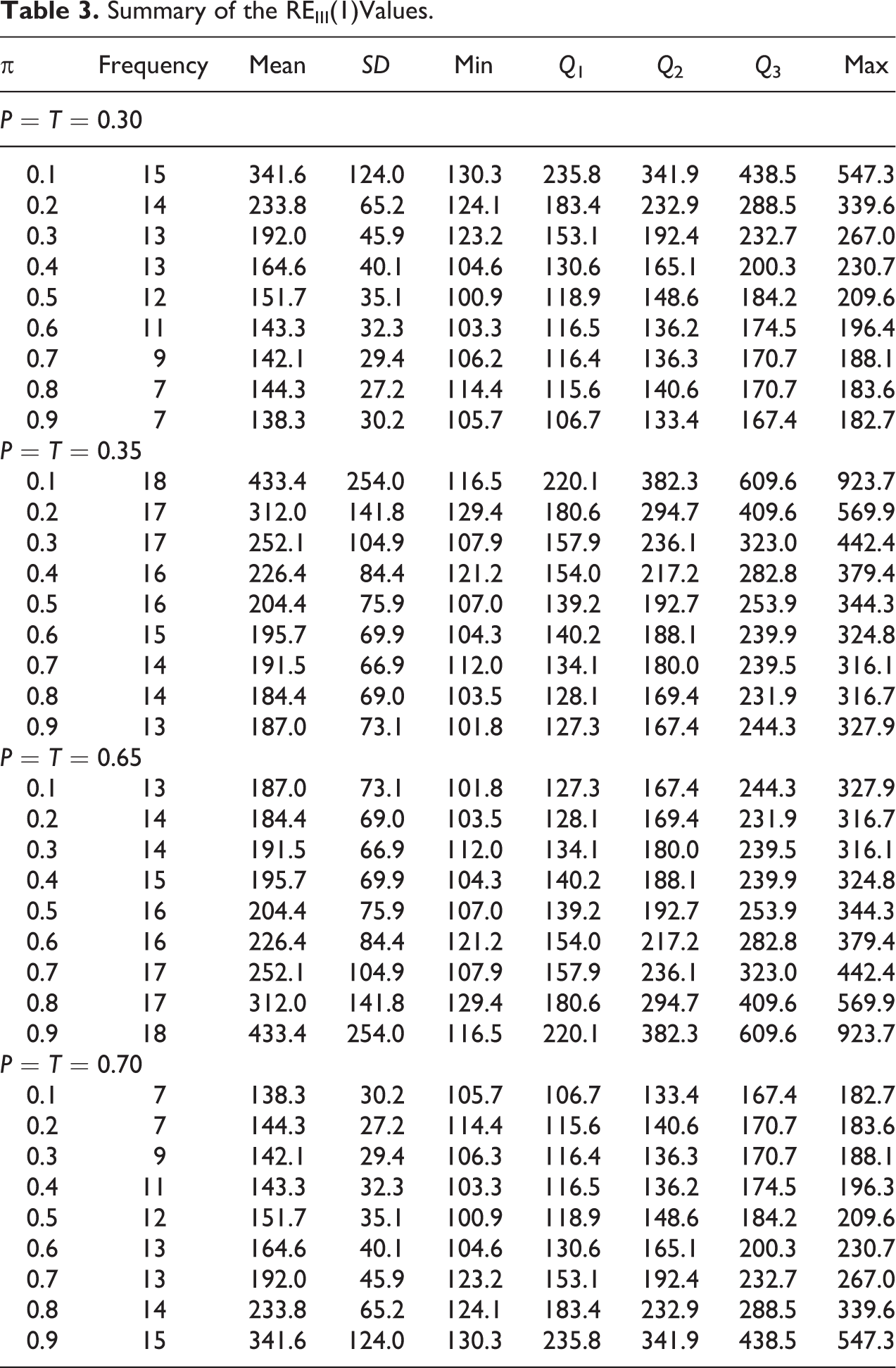
In Table 3, we present a summary of the values of the percent relative efficiency for each value of P = T and different values of π between 0.1 and 0.9.

Table 3.

Summary of the RE_III(1)Values.

π	Frequency	Mean	SD	Min	Q ₁	Q ₂	Q ₃	Max
P = T = 0.30
0.1	15	341.6	124.0	130.3	235.8	341.9	438.5	547.3
0.2	14	233.8	65.2	124.1	183.4	232.9	288.5	339.6
0.3	13	192.0	45.9	123.2	153.1	192.4	232.7	267.0
0.4	13	164.6	40.1	104.6	130.6	165.1	200.3	230.7
0.5	12	151.7	35.1	100.9	118.9	148.6	184.2	209.6
0.6	11	143.3	32.3	103.3	116.5	136.2	174.5	196.4
0.7	9	142.1	29.4	106.2	116.4	136.3	170.7	188.1
0.8	7	144.3	27.2	114.4	115.6	140.6	170.7	183.6
0.9	7	138.3	30.2	105.7	106.7	133.4	167.4	182.7
P = T = 0.35
0.1	18	433.4	254.0	116.5	220.1	382.3	609.6	923.7
0.2	17	312.0	141.8	129.4	180.6	294.7	409.6	569.9
0.3	17	252.1	104.9	107.9	157.9	236.1	323.0	442.4
0.4	16	226.4	84.4	121.2	154.0	217.2	282.8	379.4
0.5	16	204.4	75.9	107.0	139.2	192.7	253.9	344.3
0.6	15	195.7	69.9	104.3	140.2	188.1	239.9	324.8
0.7	14	191.5	66.9	112.0	134.1	180.0	239.5	316.1
0.8	14	184.4	69.0	103.5	128.1	169.4	231.9	316.7
0.9	13	187.0	73.1	101.8	127.3	167.4	244.3	327.9
P = T = 0.65
0.1	13	187.0	73.1	101.8	127.3	167.4	244.3	327.9
0.2	14	184.4	69.0	103.5	128.1	169.4	231.9	316.7
0.3	14	191.5	66.9	112.0	134.1	180.0	239.5	316.1
0.4	15	195.7	69.9	104.3	140.2	188.1	239.9	324.8
0.5	16	204.4	75.9	107.0	139.2	192.7	253.9	344.3
0.6	16	226.4	84.4	121.2	154.0	217.2	282.8	379.4
0.7	17	252.1	104.9	107.9	157.9	236.1	323.0	442.4
0.8	17	312.0	141.8	129.4	180.6	294.7	409.6	569.9
0.9	18	433.4	254.0	116.5	220.1	382.3	609.6	923.7
P = T = 0.70
0.1	7	138.3	30.2	105.7	106.7	133.4	167.4	182.7
0.2	7	144.3	27.2	114.4	115.6	140.6	170.7	183.6
0.3	9	142.1	29.4	106.3	116.4	136.3	170.7	188.1
0.4	11	143.3	32.3	103.3	116.5	136.2	174.5	196.3
0.5	12	151.7	35.1	100.9	118.9	148.6	184.2	209.6
0.6	13	164.6	40.1	104.6	130.6	165.1	200.3	230.7
0.7	13	192.0	45.9	123.2	153.1	192.4	232.7	267.0
0.8	14	233.8	65.2	124.1	183.4	232.9	288.5	339.6
0.9	15	341.6	124.0	130.3	235.8	341.9	438.5	547.3

From Table 3, the results show in the case of $P = T = 0.30$ that if $π = 0.1$ , there were 15 choices of $k_{1}$ , $r_{1}$ , and $r_{2}$ , between 1 and 3 with percent ${RE}_{III} (1)$ over 100 percent, these have: a minimum value 130.3 percent, median 341.9 percent, and maximum 547.3 percent; if $π = 0.2$ , there were 14 such choices these have: a minimum value 124.1 percent, median 232.9 percent, and maximum 339.6 percent; if $π = 0.3$ , there were 13 such values these have: a minimum value 123.2 percent, median 192.4 percent, and maximum 267.0 percent; a minimum value 104.6 percent, median 165.1 percent, and maximum 230.7 percent if $π = 0.4$ ; a minimum value 100.9 percent, median 148.6 percent, and maximum 209.6 percent if $π = 0.5$ ; a minimum value 103.3 percent, median 136.2 percent, and maximum 196.4 percent if $π = 0.6$ ; a minimum value 106.2 percent, median 136.3 percent, and maximum 188.1 percent if $π = 0.7$ ; a minimum value 114.4 percent, median 140.6 percent, and maximum 183.6 percent if $π = 0.8$ ; and a minimum value 105.7 percent, median 133.4 percent, and maximum 182.7 percent if $π = 0.9$ .

Also Table 3 shows in case $P = T = 0.3$ , that the corresponding values of the RE are 341.6 percent, 233.8 percent, 192.0 percent, 164.6 percent, 1,151.7 percent, 143.3 percent, 142.1 percent, 144.3 percent and 138.3 percent along with respective standard deviations of 124.0 percent, 65.2 percent, 45.9 percent, 40.1 percent, 35.1 percent, 32.3 percent, 29.4 percent, 27.2 percent, and 30.2 percent for π equal to 0.1, 0.2, 0.3, 0.4, 0.5, 0.6, 0.7, 0.8, and 0.9, respectively. In the same way, the rest of the results in Table 3 can be interpreted. It is interesting to see that if the value of π is close to 0, then the gain in relative efficiency of the proposed model is higher indicating that the proposed model could be more useful when the prevalence of a sensitive characteristic is not too high in a population under study. Figure 8 shows the percentage relative efficiency of the proposed fixed and targeted randomized response model with respect to the Odumade and Singh (2009) model for different values of π between 0.1 and 0.9.

Figure 8.

${RE}_{III} (1)$ values versus π between 0.1 and 0.9.

Conclusion

Thus, based on our simulation study, we conclude that the proposed new estimators can be used more efficiently and without altering the respondent’s cooperation than both Odumade and Singh (2009) and Singh and Grewal (2013) models by making a reasonable choice of parameters.

Supplemental Material

Supplemental Material, michael_paper2_updated_revised - Alternative Methods to Make Efficient Use of Two Decks of Cards in Randomized Response Sampling

Supplemental Material, michael_paper2_updated_revised for Alternative Methods to Make Efficient Use of Two Decks of Cards in Randomized Response Sampling by Michael Lee Johnson, Stephen A. Sedory, and Sarjinder Singh in Sociological Methods & Research

Footnotes

Acknowledgments

The authors are thankful to the editor in chief, Professor Christopher Winship, admin, Genevieve Butler, and two referees for their constructive comments on the original version of this article.

Declaration of Conflicting Interests

The author(s) declared no potential conflicts of interest with respect to the research, authorship, and/or publication of this article.

Funding

The author(s) received no financial support for the research, authorship, and/or publication of this article.

Supplemental Material

Supplemental material for this article is available online.

References

Chaudhuri

2011. Randomized Response and Indirect Questioning Techniques in Surveys. Boca Raton, FL: Chapman and Hall/CRC.

Chaudhuri

Christofides

T. C.

. 2013. Indirect Questioning in Sample Surveys. Berlin, Heidelberg: Springer.

Fox

J. A.

2016. Randomized Response and Related Methods: Surveying Sensitive Data. 2nd ed. CA: Sage.

Fox

J. A.

Tracy

P. E.

. 1986. Randomized Response: A Method for Sensitive Surveys. Beverly Hilss, CA: Sage.

Gjestvang

C. R.

Singh

. 2006. “A New Randomized Response Model.” Journal of the Royal Statistical Society Series B 68:523–30.

Johnson

Michael L.

2014. “Improved Randomized Response Techniques.” Unpublished manuscript, Thesis submitted to the Department of Mathematics, Texas A&M University–Kingsville, Kingsville.

Kerkvliet

1994. “Estimating a Logit Model with Randomized Data: The Case of Cocaine Use.” The Australian Journal of Statistics 36:9–20.

Kuk

A. Y. C.

1990. “Asking Sensitive Questions Indirectly.” Biomerika 77:436–38.

Lee

C.-S

Sedory

S. A.

Singh

. 2013. “Simulated Minimum Sample Sizes for Various Randomized Response Models.” Communications in Statistics: Simulation and Computation 42:771–89.

10.

Mangat

N. S.

1994. “An Improved Randomized Response Strategy.” Journal of the Royal Statistical Society: Series B 56:93–95.

11.

Mangat

N. S.

Singh

. 1990. “An Alternative Randomized Response Procedure.” Biometrika 77:439–42.

12.

Singh

2003. Advanced Sampling Theory with Applications: How Michael Selected Amy. Dordrecht, the Netherlands: Kluwer Academic.

13.

Singh

Grewal

I. S.

. 2013. “Geometric Distribution as a Randomization DEVICE Implemented to the Kuk’s Model.” International Journal of Contemporary Mathematical Sciences 8:243–48.

14.

S.-C

Sedory

S. A.

Singh

. 2015. “Kuk’s Model Adjusted for Protection and Efficiency.” Sociological Methods & Research 44:534–51.

15.

Odumade

Singh

. 2009. “Efficient Use of Two Decks of Cards in Randomized Response Sampling.” Communications in Statistics—Theory and Methods 38:439–46.

16.

Warner

S. L.

1965. “Randomized Response: A Survey Technique for Eliminating Evasive Answer Bias.” Journal of the American Statistical Association 60:63–69.

Supplementary Material

Please find the following supplemental material available below.

For Open Access articles published under a Creative Commons License, all supplemental material carries the same license as the article it is associated with.

For non-Open Access articles published, all supplemental material carries a non-exclusive license, and permission requests for re-use of supplemental material or any part of supplemental material shall be sent directly to the copyright owner as specified in the copyright notice associated with the article.

0.00 MB

2.01 MB