Using Universal Kriging to Improve Neighborhood Physical Disorder Measurement

Abstract

Ordinary kriging, a spatial interpolation technique, is commonly used in social sciences to estimate neighborhood attributes such as physical disorder. Universal kriging, developed and used in physical sciences, extends ordinary kriging by supplementing the spatial model with additional covariates. We measured physical disorder on 1,826 sampled block faces across four U.S. cities (New York, Philadelphia, Detroit, and San Jose) using Google Street View imagery. We then compared leave-one-out cross-validation accuracy between universal and ordinary kriging and used random subsamples of our observed data to explore whether universal kriging could provide equal measurement accuracy with less spatially dense samples. Universal kriging did not always improve accuracy. However, a measure of housing vacancy did improve estimation accuracy in Philadelphia and Detroit (7.9 percent and 6.8 percent lower root mean square error, respectively) and allowed for equivalent estimation accuracy with half the sampled points in Philadelphia. Universal kriging may improve neighborhood measurement.

Keywords

cities physical disorder spatial analysis universal kriging urban health

Introduction

Physical Disorder, Health, and Society

Exposure to physical disorder—visual indications of urban deterioration such as litter, graffiti, vacant lots, and abandoned buildings (Raudenbush and Sampson 1999; Skogan 2015)—is of great interest in the social and population health sciences. Most famously, the controversial “broken windows” theory that physical disorder encourages violent crime has been intensely scrutinized in the popular and academic press (Cerdá et al. 2009; Sampson and Raudenbush 2004; J. Q. Wilson and Kelling 1982; Wilcox et al. 2004). Moreover, disorder has been linked to sexually transmitted disease independent of poverty, perhaps because a dilapidated environment encourages high-risk sexual behavior (Cohen et al. 2000; Latkin et al. 2007). Latkin and Curry (2003) further proposed that exposure to disorder might cause depression, a finding that has been subsequently explored extensively (Browning et al. 2013; Hill, Ross, and Angel 2005; Joshi et al. 2017; Mair, Roux, and Galea 2008). More broadly, exposure to physical disorder may induce fear and distress (C. E. Ross and Mirowsky 2009, 2001; Theall et al. 2013), with consequent harms both to social ties and to personal health.

Policy makers, including public health authorities (Australian Local Government Association 2006; Centers for Disease Control and Prevention 2012), have an interest in physical disorder because it can be addressed through policies that, for example, green vacant lots (Branas et al. 2011) or implement graffiti or blight removal programs (Eagle 2007; Tavares 2014). Evidence of the benefits of program has been limited in part by the difficulty of obtaining accurate measurements of disorder (Skogan 2015), especially in light of potentially serious implications of broken windows policing (e.g., Duneier and Carter 1999). Broadly, the link between physical disorder and health-relevant behaviors has been inconsistent (Hoehner et al. 2005; Laraia et al. 2007; Mendes de Leon et al. 2009; Strath et al. 2012), and thus refinement of disorder estimates using available data may help to resolve or explain such inconsistencies.

Measuring Physical Disorder

One common approach to measuring disorder is to ask subjects to report their perceptions of disorder indicators in their local environment (e.g., C. E. Ross and Mirowsky 1999). Indeed, understanding perceptions of and behavioral response to different contexts is vital for informing place-based health promotion strategies (Blacksher and Lovasi 2012). Yet, because relying on self-report alone to characterize the environment may result in same-source bias (Avolio, Yammarino, and Bass 1991; Duncan and Raudenbush 1999), researchers often complement or supplant self-reported perceived measures with neighborhood measures reported by nearby residents (Mujahid et al. 2007, 2011) or trained neighborhood auditors (Reiss 1971; Sampson and Raudenbush 1999).

There are several approaches to such independent neighborhood measurement. Some studies assess only the residential block of subjects whose health is being studied (e.g., Franzini et al. 2008; Kimbro, Brooks-Gunn, and McLanahan 2011; Kwarteng et al. 2014), which can be efficient if a neighborhood audit is added to a home visit protocol but does not capture the broader surrounding context that is relevant to behaviors and health (Bader and Ailshire 2014) and typically precludes straightforward use of remote imagery for the audit (Bader, Mooney, and Rundle 2016). However, because auditing all blocks describing a subject’s neighborhood is usually prohibitively expensive (though not always; Strath et al. 2012), many studies aiming to characterize neighborhood physical disorder audit a random sample of blocks (King 2008; Sampson and Raudenbush 1999), in some cases using geostatistical tools to interpolate between sampled points (Auchincloss et al. 2007; Bader and Ailshire 2014; Keyes et al. 2012; Mooney et al. 2014).

Interpolating Physical Disorder Measures

One common geostatistical interpolation technique is ordinary kriging (Cressie 1988). Ordinary kriging takes advantage of spatial autocorrelation between observations (i.e., that closer measurements tend to be more similar) to estimate both a value and an estimate of error in that value estimate at unobserved locations. However, ordinary kriging does not account for between-location variation in small-scale geographic features such as street size or jurisdictional boundaries that might be correlated with indicators of the attributes of interest (Bader and Ailshire 2014). This can lead to error in imputed neighborhood traits. For example, because pedestrians create litter, urban streets with more retail activity and consequently more pedestrian traffic may have more litter on average, independent of other sources of disorder (Lovasi et al. 2012). Ordinary kriging cannot incorporate measures of retail activity such as street classification or retail floor area into disorder interpolations.

One alternative to ordinary kriging is land-use regression (Shmool et al. 2014). Land-use regression uses covariates measured at observed points to estimate what would be observed at other locations where covariates have been observed but the measure of interest has not (Z. Ross et al. 2007). For example, a land-use regression model for physical disorder might use observation-specific measurements such as owner occupancy (because owner-occupied homes tend to be better maintained; Sweeney 1974) at observed locations to predict physical disorder at unobserved locations. Prior work has shown land-use regression to perform better than ordinary kriging for spatial measures with considerable small-scale variation or where the source of the measured construct is known and well measured (e.g., traffic as a predictor of air pollution; Briggs et al. 2000; Hoek et al. 2008). However, land-use regression does not perform as well in contexts where land use is not strongly tied to the measure of interest, as may be expected for physical disorder. Moreover, the information that an unobserved location might be near observed locations where high levels of disorder were observed would be lost in a pure land-use regression model (Z. Ross et al. 2006). Thus, both land-use regression and ordinary kriging use only part of the information that might be available to base interpolations upon.

Universal kriging is an interpolation technique that incorporates both spatial correlation between observations and measured covariates in the same prediction model (Stein and Corsten 1991). For example, a universal kriging model can be fitted to spatial data wherein each point in the sample includes a location, a level of physical disorder, and covariates such as population density in the census block group where the sample was taken. Estimates at unobserved locations would then be made by first estimating the level of disorder as in ordinary kriging, then modeling the residual as a function of measured characteristics at observation locations and “correcting” for the difference. In principle, this approach should improve estimation accuracy at unobserved locations if the measured characteristic incorporates additional information about the level of disorder beyond what can be inferred from autocorrelation of the measured points alone (Hengl, Heuvelink, and Stein 2003). However, to the best of our knowledge, while universal kriging has been used in research regarding health-relevant air quality metrics (Clougherty et al. 2013), it has not been explored as a way to improve accuracy of neighborhood disorder estimates.

In this article, we compare estimation accuracy using ordinary kriging to estimation accuracy using universal kriging to incorporate readily available U.S. Census measures such as population density and housing vacancy to interpolate a measure of neighborhood disorder. We address two aspects of universal kriging. First, we examine the degree to which universal kriging including covariates from free sources of data improves the interpolated values of neighborhood conditions over ordinary kriging. Second, we examine whether universal kriging can reduce the sample size necessary to interpolate values at nonsampled locations. These analyses can help researchers create more accurate and cost-effective designs to measure neighborhood conditions.

Method

Disorder Observations

For this investigation, we employed measures of neighborhood disorder in New York, NY; Philadelphia, PA; Detroit, MI; and San Jose, CA. The construction and validation of the measure against data from the 2010 decennial U.S. Census has been described in detail elsewhere (Mooney et al. 2014) and validated in Detroit against a neighborhood disorder measure constructed using in-person audits roughly one year earlier (Mooney et al. 2017). Briefly, we sampled block faces in a grid across each city with oversamples corresponding to areas of greater researcher interest, generally more densely populated and deprived areas. On each of the 1,826 block faces in the final sample, trained street auditors used the computer-assisted neighborhood visual assessment system (Bader et al. 2015) and imagery from Google Street View (Anguelov et al. 2010; Badland et al. 2010; Rundle et al. 2011; J. S. Wilson et al. 2012) to measure presence of litter, empty bottles, graffiti, abandoned cars, poor building conditions, burned out buildings, boarded up buildings, vacant lots, and buildings with bars on windows. These items, whose presence on any given block face is time dependent, nonetheless reliably recur in more generally disordered spatial contexts (Mooney et al. 2014; Raudenbush and Sampson 1999). These items were combined in an “ecometric” measurement scale using a multilevel item-response model with items nested within street segments with coefficients measuring the “severity” of items (Raudenbush and Sampson 1999). Less severe indicators of disorder such as litter were nearly ubiquitous whereas more severe indicators such as abandoned buildings were very rare, but presence of more severe indicators generally implied presence of less severe indicators as well. Mean disorder was highest in Detroit, lowest in San Jose, and roughly equivalent in New York and Philadelphia (for more detail, see Mooney et al. 2014). The resulting scale had an internal consistency reliability score of 0.93.

Covariate Observations

Because our primary goal was to assess whether we could improve accuracy of spatial models by incorporating a free, readily available source of data, our primary spatially located covariates were economic and demographic measures taken from the U.S. Census. We obtained 2010 decennial U.S. Census measures of population density, housing vacancy, and proportion of owner-occupied housing units occupied for each census block group. We selected population density because it is a driver of high pedestrian volume, which contributes to some indicators of disorder (Lovasi et al. 2012). We selected housing vacancy because vacant homes are frequently poorly maintained or subject to defacement, and because vacant buildings are sometimes considered an indicator of disorder in themselves (Skogan 2015). Finally, we selected owner-occupied housing because of evidence from real-estate economics that owner-occupied housing tends to be better maintained (Sweeney 1974). For the census measures, we selected block groups because they were the smallest spatial unit for which these census data were available. To conduct a sensitivity analysis, we also obtained all measures at the census tract level. As compared with block groups, tracts are larger spatial units, each containing at least one and usually several block groups. Tracts tend to be more heterogeneous than block groups (Iceland and Steinmetz 2003), and thus may convey less information for a universal kriging model.

Kriging

Ordinary kriging assumes intrinsic stationarity—that is, the spatial process (i.e., the social processes generating disorder) has a constant mean across the area for which the data are being interpolated, while the covariance between pairs of points depends only on the distance between the points (Cressie 1988). By contrast, universal kriging allows the spatial process to include an underlying trend (or “drift” in the geostatistical literature) that can be described by a linear function of predictors and assumes intrinsic stationarity only after accounting for this underlying trend (Pebesma 2006). For physical disorder, as noted in the Introduction section, we anticipate that social processes such as neighborhood abandonment are spatially patterned and may be explained by measured covariates, thus suggesting universal kriging may improve interpolation performance. All kriging techniques allow estimation of error surrounding the estimated value.

To quantify the incremental accuracy improvement afforded by incorporating covariates into the kriging model, we used leave-one-out (also known as jackknife) cross-validation to estimate the root mean squared error (RMSE) from each model (Bivand et al. 2008). That is, for each observation, we used all other observations to predict what that observation would be, then considered the difference between the model’s prediction and the actual observation to represent the error in that location. Lower RMSE scores thus indicate improved model accuracy. The kriging process requires fitting a function estimating variance between observations as a function of distance between observations (the “lag distance”; Bader and Ailshire 2014). Such functions can be fit visually or algorithmically; fitting visually allows more flexibility to minimize error at different spatial distances but fitting algorithmically limits subjectivity and error due to human input (Cressie 1985). We fit all variograms algorithmically using the Levenberg–Marquardt algorithm (Moré 1978).

Because kriging uses point locations, we assigned each block face observation the coordinates of the point midway between the blocks end points. We then assigned each point the characteristics of the census block group in which it was embedded. However, not all census measures were available for each sampled location. For example, the census provides no information regarding owner occupancy of the nonresidential tract that comprises Philadelphia International Airport. While these census data were missing for only 17 block faces (1 percent of all audited block faces), we wanted to retain maximal comparability between models. We decided that since only observations in residential census tracts without missing data would be used for our universal kriging, this should be balanced by a version of the ordinary kriging restricted to the same subset of observations. We therefore computed two RMSEs for ordinary kriging: one using all sampling points to represent the real-world ordinary kriging error and the other using only the sample points for which census data were available to be more directly comparable to universal kriging models.

In all, we computed five cross-validated measures for each city using: (1) ordinary kriging, (2) ordinary kriging only for the sample points where all census data were available, (3) universal kriging incorporating population density as a predictor, (4) universal kriging incorporating housing vacancy as a predictor, and (5) universal kriging incorporating proportion of housing units occupied by owners as a predictor.

Sampling Density

In addition to improving estimation accuracy for a fixed sample density, incorporating covariates might allow equally accurate models at decreased sample density because the incorporated covariates provide additional information at unmeasured locations. To assess the benefits of universal kriging for the sensitivity of model accuracy to sampling density, we compared the decrease in accuracy from each kriging approach with smaller samples within Philadelphia. Specifically, we first randomly selected a 90 percent subset of sample points and computed the RMSE for the resulting model. We then repeated this procedure for progressively smaller random subsets from 80 percent to 10 percent. We repeated this random subsetting procedure 100 times for a total of 800 models fitted for each approach. We then used Wilcoxon rank-sum tests to identify presence of improvement in accuracy at each level of sample density. For this analysis, we tested accuracy of prediction using two covariates: population density and housing vacancy.

Software

All analyses used R for Windows Version 3.2.3 (Vienna, Austria), including the “geoR version 1.7-5.2,” “gstat version 1.1-5,” and “rgdal version 1.1-10” packages for spatial analysis and “ggplot2 version 2: 2.2.1” to construct the figure (Pebesma 2004; Pebesma and Bivand 2005; Ribeiro and Diggle 2001; Wickham 2009).

Results

The characteristics of each block face sample in each city are presented in Table 1. The four cities covered a diverse profile of urban form and economic prosperity. Whereas New York and San Jose represent extremes of population density, both are only minimally abandoned. Philadelphia represented a middle ground on the measures of interest in this study.

Table 1.

Selected Characteristics of the Block Face Sample for Each City.

City	Audited Segments	Segments With Census Data (Total Percentage)	Population Density per Square Mile (Median, IQR)	Percent Vacant (Median, IQR)	Percent Owner Occupied (Median, IQR)
New York	532	520 (98)	51,982 (28,411–81,251)	6 (4–8)	23 (9–47)
Detroit	503	500 (100)	6,567 (5,193–7,712)	22 (17–27)	56 (49–63)
Philadelphia	502	500 (100)	18,983 (14,047–24,595)	11 (7–15)	54 (45–63)
San Jose	289	289 (100)	2,903 (2,408–3,549)	3 (3–4)	61 (40–73)

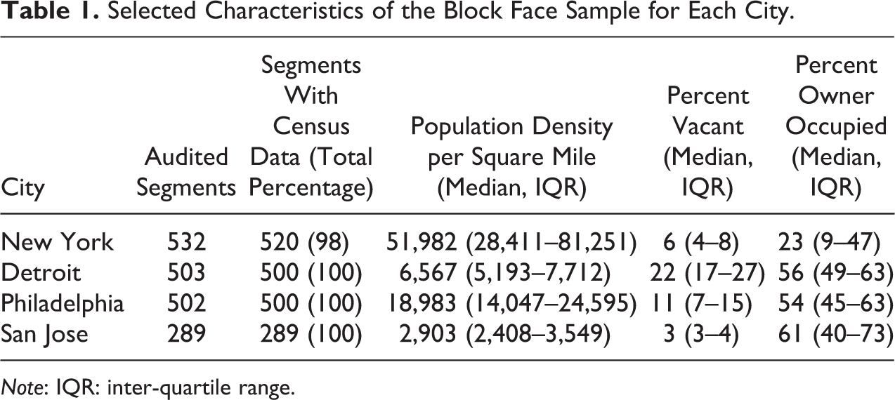
Note: IQR: inter-quartile range.

Kriging accuracy varied much more between cities than between kriging methods (Table 2). New York had the best prediction accuracy for all models (RMSE = .288 for ordinary kriging), while Detroit had the worst (RMSE = .595 for ordinary kriging). Universal kriging incorporating block group–level measures modestly improved estimation accuracy in most, though not all, instances. Of the covariates tested, housing vacancy was the most effective at increasing accuracy, particularly in Detroit and Philadelphia (6.8 percent and 7.9 percent improved accuracy, respectively), and population density added the least information (no more than 1.4 percent improved accuracy) in each city. Estimation accuracy improvement was more modest using covariates taken from the point’s census tract rather than its census block group (Online Supplemental Appendix Table S1). Maps generated from ordinary kriging resulted in fewer, smoother clusters of disorder than those generated using universal kriging (Figure 1).

Table 2.

Cross-validation Results Evaluating Improvement in In-sample Prediction Accuracy Achieved When Incorporating Covariates in Universal Kriging Model.

	New York, NY		Detroit, MI		Philadelphia, PA		San Jose, CA
Geographic Feature Included as a Universal Kriging Covariate	RMSE	Percentage of Improvement (Percent)	RMSE	Percentage of Improvement (Percent)	RMSE	Percentage of Improvement (Percent)	RMSE	Percentage of Improvement (Percent)
Ordinary kriging
All sample points	.288	—	.595	—	.441	—	.326	—
Points with census data	.286	0.7	.581	2.3	.439	0.3	.326	0.0
Population density in block group	.286	0.8	.587	1.4	.440	0.1	.325	0.4
Percent vacant in block group	.283	1.7	.555	6.8	.406	7.9	.342	−4.8
Owner-occupied housing	.289	−0.3	.570	4.2	.432	1.9	.318	2.6

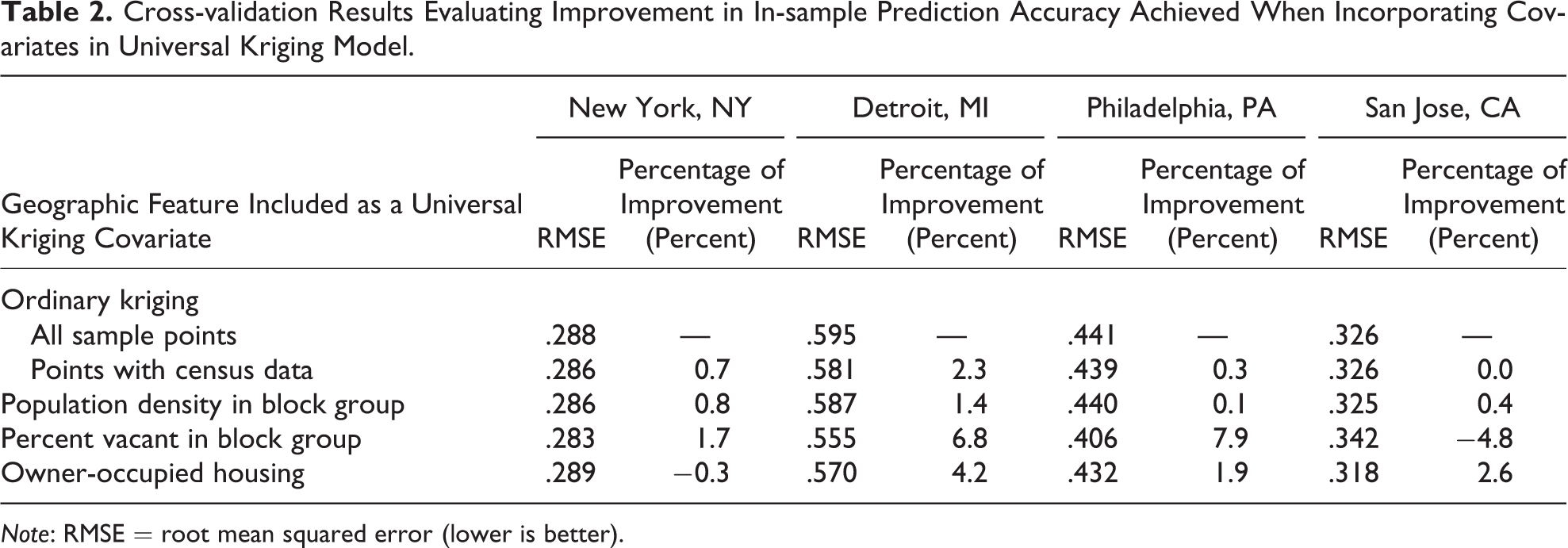
Note: RMSE = root mean squared error (lower is better).

Figure 1.

Maps of census tracts in Philadelphia. The left panel shows mean physical disorder in each tract computed using ordinary kriging, the middle panel shows physical disorder computed using universal kriging incorporating 2010 U.S. Census data on housing vacancy as a covariate, and the right panel shows 2010 U.S. Census data on housing vacancy for each tract.

In the context in which universal kriging was most successful at reducing error in the overall sample, for housing vacancy in Philadelphia, universal kriging also substantially reduced the sampling density necessary to achieve a given accuracy (Figure 2, Online Supplemental Appendix Table S2). For example, with only 200 sample points (40 percent of the full sample) incorporated in the kriging model, the median RMSE in the universal kriging model was .438, lower than the .439 RMSE for ordinary kriging for the full sample (Wilcoxon rank-sum test, p value < .01).

Figure 2.

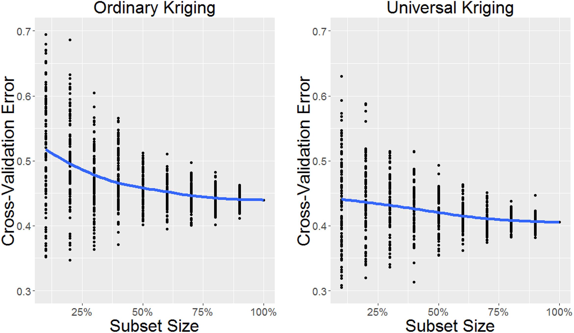
Comparison of the empirical error in kriging models and size of the subset sample. Universal kriging with percentage of vacancy was not only more accurate overall but also reduced the number of sample points needed to achieve a given accuracy as compared with ordinary kriging.

However, incorporating population density, a covariate that did not substantially improve the model in the full sample, into the universal kriging model in Philadelphia did not reduce the sample size needed to achieve a given accuracy (Online Supplemental Appendix Figure S1).

Discussion

Reducing error in the measures used to quantify neighborhood environment characteristics can increase researchers’ ability to identify associations between neighborhood conditions and health outcomes. In this analysis of small-scale spatial patterns of physical disorder, we compared the estimation accuracy of universal kriging incorporating readily available U.S. Census measures to that of ordinary kriging. Incorporating a census measure of housing vacancy modestly improved estimation accuracy in Philadelphia and Detroit, cities with substantial areas of abandonment, but universal kriging did not uniformly improve accuracy across multiple measures in four cities. A measure that was effective in improving accuracy in Philadelphia, housing vacancy, was also effective in achieving equal or better accuracy with less dense samples in Philadelphia.

We found that both the theoretical relevance of the covariates included in models and the context in which disorder was being estimated had strong impacts on model accuracy. Housing vacancy, the covariate that most improved accuracy, is conceptually similar to neighborhood abandonment, which is a key driver of physical disorder (Sampson and Raudenbush 1999; Skogan 2015). The fact that housing vacancy measures did not substantially improve accuracy in New York and San Jose likely is consistent with very low vacancy rates throughout those cities, as shown in Table 1. Future research might productively explore the availability of and benefits of various forms of spatially located covariates more systematically, analogous to a genome-wide association study (Ioannidis et al. 2009). Understanding which covariates are most informative in which contexts may be particularly valuable as spatially located administrative data sets become increasingly available and as spatial tools develop to make “Big Data” analyses incorporating such data sets simpler (Mooney, Westreich, and El-Sayed 2015). “Blind kriging” is one approach to interpolation using empirical rather than a priori covariate selection and has been explored in the computer simulation and materials design literature, but to our knowledge not explored in social sciences (Joseph, Hung, and Sudjianto 2008).

The present study focused on demonstrating the advantages of universal kriging for a measure of neighborhood physical disorder. In principle, universal kriging is well suited to measures with microscale variation that ordinary kriging cannot account for but that also demonstrate spatial autocorrelation that covariates incorporated in land-use regression cannot account for. For example, universal kriging might be appropriate for estimating prevalence of informal street vendors (Lucan et al. 2013), whose locations are both affected by street scale and by broader neighborhood conditions, or tree pollen counts (Weinberger, Kinney, and Lovasi 2015), which are affected by proximity to individual trees, proximity to parks (which typically have different tree species than streets), and prevailing wind patterns. Broadly speaking, accurate measurement of contextual factors that vary within a city can be used to inform spatially targeted public health interventions and to coordinate a multisectoral response to address any health hazards in the environment.

However, it is important to note that universal kriging models performed worse than ordinary kriging models in some cases. In kriging models as in all statistical models, incorporating additional information increases the risk of model overfitting (Box 1976). Additionally, universal kriging, unlike ordinary kriging, allows interpolations to exceed the observed range of the data and could, therefore, increase the error of the interpolations if the covariates are not well specified. A prior study of air pollution found ordinary kriging to be prone to biases due to overfit models (Parmentier et al. 2014); by incorporating more information, universal kriging may raise this risk. A poorly specified measurement model will affect the accuracy of measures. For example, in San Jose, population density does not vary much across observed locations and does not inform the model. Universal kriging, unlike ordinary kriging, allows for estimates outside of the observed range of observations and thus introduces error not included in the ordinary kriging model. Broadly, we expect that universal kriging will improve measure accuracy when (a) the covariate varies across spatial units, (b) that variation is spatially correlated with the measure being interpolated, and (c) the spatial correlation between the covariate and the measure exists at a smaller scale than the spatial density of the sample.

Our analysis showed that universal kriging with appropriate covariates helped reduce the sampling error and sampling variance over ordinary kriging. In practice, this indicates that well-selected covariates can reduce the spatial density of samples required to interpolate values of disorder and other characteristics. The reduction in sampling density could be especially important for studies that rely on in-person audits where transportation to and from sampled locations makes up a substantial fraction of study costs (Mooney et al. 2017).

In data science research focusing on accurate prediction, recent studies suggest promising fixes to overfitting by incorporating machine learning–derived algorithmic model fitting with tunable penalty parameters (Tibshirani 1996). Tunable models are particularly appropriate when estimation rather than inference is the goal of the modeling exercise (Breiman 2001), as is the case for spatial estimation of neighborhood measures. Penalized universal kriging models with many covariates may be a promising area for future research.

This study had several notable strengths. Most importantly, our data set included data from four cities which have very different economic and spatial profiles, so our results are relatively robust to city-specific artifacts. More broadly, the relatively large spatial sample of assessed block faces provided a solid base with which to explore sample size variability.

Limitations of this work include the lack of a gold standard benchmark. In practice, there is no single optimal measure of disorder (Skogan 2015); future work on disorder measurement might focus on alternate methods of triangulation that incorporate big data disorder indicators such as 311 calls (Mooney et al. 2015) and consider the potential for locale-dependent measurement error (as when an auditor familiar with a given context can distinguish better between a street mural and graffiti in that context than he or she might in another context; Bader et al. 2015; Phillips et al. 2017). Future work estimating the value of various types of kriging models would also benefit from simulation studies using observational data for which true values are known. Another limitation is that the relevant scale for neighborhood disorder is likely different from that of other health-relevant constructs such as air pollution or pedestrian activity; thus, our finding on the value of universal kriging may not generalize to other neighborhood measures. Our use of census data brings several limitations. First, census data capture only variability between block groups, leaving variability within block groups as a source of error. Second, census data likely capture only some of the underlying drift in physical disorder levels; barriers such as highways or rivers might be larger determinants of spatial variation in disorder. Future work should investigate the use of distance metrics for kriging variograms that incorporate a distance penalty for crossing such a barrier. Finally, we used an algorithm to fit kriging functions to variograms in order to avoid biases in the comparison, but in practice, fitting variograms by eye is often recommended. Thus, our comparison may not replicate the true trade-off facing a spatial analyst interested in interpolating a physical disorder measure.

Conclusions

Universal kriging incorporating relevant spatially located covariates improved model estimation accuracy for one measure of neighborhood physical disorder. This improved accuracy leveraged preexisting data and required no additional audit time. Figure 3 is a flowchart of how secondary data, universal kriging, and cross-validation could be used to improve neighborhood measure interpolation. Broadly, universal kriging holds promise for improved interpolation of neighborhood environmental measures in future research on social conditions. Our work serves as a demonstration of universal kriging in general, but additional investigation will be needed to identify the measures, covariates, and spatial scales for which universal kriging can most improve the measurement of neighborhood conditions.

Figure 3.

A potential workflow for researchers considering using universal kriging to improve neighborhood measurement. This workflow could be used either with pilot data to estimate the sample density needed using a suitable universal kriging covariate or with final data to improve the final measurement model.

Supplemental Material

Supplemental Material, UniversalKriging_SMR_Supplemental_Content - Using Universal Kriging to Improve Neighborhood Physical Disorder Measurement

Supplemental Material, UniversalKriging_SMR_Supplemental_Content for Using Universal Kriging to Improve Neighborhood Physical Disorder Measurement by Stephen J. Mooney, Michael D. M. Bader, Gina S. Lovasi, Kathryn M. Neckerman, Andrew G. Rundle and Julien O. Teitler in Sociological Methods & Research

Footnotes

Declaration of Conflicting Interests

The author(s) declared no potential conflicts of interest with respect to the research, authorship, and/or publication of this article.

Funding

The author(s) disclosed receipt of the following financial support for the research, authorship, and/or publication of this article: This work was supported by Eunice Kennedy Shriver National Institute of Child Health and Human Development grant 5T32HD057833-07.

Supplemental Material

Supplemental material for this article is available online.

References

Anguelov

Dragomir

Dulong

Carole

Filip

Daniel

Frueh

Christian

Lafon

Stéphane

Lyon

Richard

Ogale

Abhijit

Vincent

Luc

Weaver

Josh

. 2010. “Google Street View: Capturing the World at Street Level.” Computer 43(6):32–38.

Auchincloss

Amy H.

Roux

Ana V. Diez

Brown

Daniel G.

Raghunathan

Trivellore E.

Erdmann

Christine A.

. 2007. “Filling the Gaps: Spatial Interpolation of Residential Survey Data in the Estimation of Neighborhood Characteristics.” Epidemiology (Cambridge, Mass.) 18:469.

Australian Local Government Association. 2006. Age-friendly Built Environments: Opportunities for Local Government. Deakin, Australia: Australian Local Government Association.

Avolio

Bruce J.

Yammarino

Francis J.

Bass

Bernard M.

. 1991. “Identifying Common Methods Variance With Data Collected From a Single Source: An Unresolved Sticky Issue.” Journal of Management 17:571–87.

Bader

Michael D. M.

Ailshire

Jennifer A.

. 2014. “Creating Measures of Theoretically Relevant Neighborhood Attributes at Multiple Spatial Scales.” Sociological Methodology 44(1):322–68. doi: 10.1177/0081175013516749.

Bader

Michael D. M.

Mooney

Stephen J.

Lee

Yeon Jin

Sheehan

Daniel

Neckerman

Kathryn M.

Rundle

Andrew G.

Teitler

Julien O.

. 2015. “Development and Deployment of the Computer Assisted Neighborhood Visual Assessment System (CANVAS) to Measure Health-related Neighborhood Conditions.” Health and Place 31:163–72.

Bader

Michael D. M.

Mooney

Stephen J.

Rundle

Andrew G.

. 2016. “Protecting Personally Identifiable Information When Using Online Geographic Tools for Public Health Research.” American Journal of Public Health 106:206–8.

Badland

H. M.

Opit

Witten

Kearns

R. A.

Mavoa

. 2010. “Can Virtual Streetscape Audits Reliably Replace Physical Streetscape Audits?” Journal of Urban Health-Bulletin of the New York Academy of Medicine 87:1007–16.

Bivand

Roger S.

Pebesma

Edzer J.

Gomez-Rubio

Virgilio

Pebesma

Edzer Jan

. 2008. Applied Spatial Data Analysis With R. Vol. 747248717. New York: Springer.

10.

Blacksher

Lovasi

G. S.

. 2012. “Place-focused Physical Activity Research, Human Agency, and Social Justice in Public Health: Taking Agency Seriously in Studies of the Built Environment.” Health Place 18:172–9.

11.

Box

George E. P.

1976. “Science and Statistics.” Journal of the American Statistical Association 71:791–99.

12.

Branas

Charles C.

Cheney

Rose A.

MacDonald

John M.

Tam

Vicky W.

Jackson

Tara D.

Ten Have

Thomas R.

. 2011. “A Difference-in-differences Analysis of Health, Safety, and Greening Vacant Urban Space.” American Journal of Epidemiology 174:1296.

13.

Breiman

Leo

. 2001. “Statistical Modeling: The Two Cultures (With Comments and a Rejoinder by the Author).” Statistical Science 16:199–231.

14.

Briggs

David J.

Hoogh

Cornelis de

Gulliver

John

Wills

John

Elliott

Paul

Kingham

Simon

Smallbone

Kirsty

. 2000. “A Regression-based Method for Mapping Traffic-related Air Pollution: Application and Testing in Four Contrasting Urban Environments.” Science of the Total Environment 253:151–67.

15.

Browning

Christopher R.

Soller

Brian

Gardner

Margo

Brooks-Gunn

Jeanne

. 2013. “‘Feeling Disorder’ as a Comparative and Contingent Process Gender, Neighborhood Conditions, and Adolescent Mental Health.” Journal of Health and Social Behavior 54:296–314.

16.

Centers for Disease Control and Prevention. 2012. “Healthy Aging & the Built Environment.” Retrieved April 2018. (https://www.cdc.gov/healthyplaces/healthtopics/healthyaging.htm).

17.

Cerdá

Magdalena

Tracy

Melissa

Messner

Steven F.

Vlahov

David

Tardiff

Kenneth

Galea

Sandro

. 2009. “Misdemeanor Policing, Physical Disorder, and Gun-related Homicide: A Spatial Analytic Test of ‘Broken-windows’ Theory.” Epidemiology 20:533–41.

18.

Clougherty

Jane E.

Kheirbek

Iyad

Eisl

Holger M.

Ross

Zev

Pezeshki

Grant

Gorczynski

John E.

Johnson

Sarah

Markowitz

Steven

Kass

Daniel

Matte

Thomas

. 2013. “Intra-urban Spatial Variability in Wintertime Street-level Concentrations of Multiple Combustion-related Air Pollutants: The New York City Community Air Survey (NYCCAS).” Journal of Exposure Science and Environmental Epidemiology 23:232–40.

19.

Cohen

Spear

Scribner

Kissinger

Mason

Wildgen

. 2000. “‘Broken Windows’ and the Risk of Gonorrhea.” American Journal of Public Health 90:230–6.

20.

Cressie

Noel

. 1985. “Fitting Variogram Models by Weighted Least Squares.” Journal of the International Association for Mathematical Geology 17:563–86.

21.

Cressie

Noel

. 1988. “Spatial Prediction and Ordinary Kriging.” Mathematical Geology 20:405–21.

22.

Duncan

Greg J.

Raudenbush

Stephen W.

. 1999. “Assessing the Effects of Context in Studies of Child and Youth Development.” Educational Psychologist 34:29–41.

23.

Duneier

Mitchell

Carter

Ovie

. 1999. Sidewalk. New York: Farrar, Straus, and Giroux.

24.

Eagle

Steven J

. 2007. “Does Blight Really Justify Condemnation?” The Urban Lawyer 39:833–58.

25.

Franzini

Luisa

Caughy

Margaret O’Brien

Nettles

Saundra Murray

O’Campo

Patricia

. 2008. “Perceptions of Disorder: Contributions of Neighborhood Characteristics to Subjective Perceptions of Disorder.” Journal of Environmental Psychology 28:83–93.

26.

Hengl

Tomislav

Heuvelink

Gerard B. M.

Stein

Alfred

. 2003. “Comparison of Kriging With External Drift and Regression-kriging.” Technical Note, International Institute for Geo-information Science and Earth Observation (ITC). Retrieved April 2018. (https://webapps.itc.utwente.nl/librarywww/papers_2003/misca/hengl_comparison.pdf).

27.

Hill

Terrence D.

Ross

Catherine E.

Angel

Ronald J.

. 2005. “Neighborhood Disorder, Psychophysiological Distress, and Health.” Journal of Health and Social Behavior 46:170–86.

28.

Hoehner

Christine M.

Ramirez

Laura K. Brennan

Elliott

Michael B.

Handy

Susan L.

Brownson

Ross C.

. 2005. “Perceived and Objective Environmental Measures and Physical Activity Among Urban Adults.” American Journal of Preventive Medicine 28:105–16.

29.

Hoek

Gerard

Beelen

Rob

Hoogh

Kees De

Vienneau

Danielle

Gulliver

John

Fischer

Paul

Briggs

David

. 2008. “A Review of Land-use Regression Models to Assess Spatial Variation of Outdoor Air Pollution.” Atmospheric Environment 42:7561–78.

30.

Iceland

John

Steinmetz

Erika

. 2003. “The Effects of Using Census Block Groups Instead of Census Tracts When Examining Residential Housing Patterns.” Bureau of the Census 5.

31.

Ioannidis

John P. A.

Yun Loy

Poulton

Richie

Chia

Kee Seng

. 2009. “Researching Genetic Versus Nongenetic Determinants of Disease: A Comparison and Proposed Unification.” Science Translational Medicine 1:7ps8.

32.

Joseph

V. Roshan

Hung

Ying

Sudjianto

Agus

. 2008. “Blind Kriging: A New Method for Developing Metamodels.” Journal of Mechanical Design 130:1–8.

33.

Joshi

Spruha

Mooney

Stephen J.

Rundle

Andrew G.

Quinn

James W.

Beard

John B.

Cerda

Magdalena

. 2017. “Pathways From Neighborhood Poverty to Depression Among Older Adults.” Health & Place 43:138–43

34.

Keyes

Katherine M.

McLaughlin

Katie A.

Koenen

Karestan C.

Goldmann

Emily

Uddin

Monica

Galea

Sandro

. 2012. “Child Maltreatment Increases Sensitivity to Adverse Social Contexts: Neighborhood Physical Disorder and Incident Binge Drinking in Detroit.” Drug and Alcohol Dependence 122:77–85.

35.

Kimbro

Rachel Tolbert

Brooks-Gunn

Jeanne

McLanahan

Sara

. 2011. “Young Children in Urban Areas: Links Among Neighborhood Characteristics, Weight Status, Outdoor Play, and Television Watching.” Social Science and Medicine 72:668–76.

36.

King

Diane

. 2008. “Neighborhood and Individual Factors in Activity in Older Adults: Results From the Neighborhood and Senior Health Study.” Journal of Aging and Physical Activity 16:144–70.

37.

Kwarteng

Jamila L.

Schulz

Amy J.

Mentz

Graciela B.

Zenk

Shannon N.

Opperman

Alisha A.

. 2014. “Associations Between Observed Neighborhood Characteristics and Physical Activity: Findings From a Multiethnic Urban Community.” Journal of Public Health 36:358–67.

38.

Laraia

Barbara

Messer

Lynne

Evenson

Kelly

Kaufman

Jay S.

. 2007. “Neighborhood Factors Associated With Physical Activity and Adequacy of Weight Gain During Pregnancy.” Journal of Urban Health 84:793–806.

39.

Latkin

Carl A.

Curry

Aaron D.

. 2003. “Stressful Neighborhoods and Depression: A Prospective Study of the Impact of Neighborhood Disorder.” Journal of Health and Social Behavior 44(1):34–44.

40.

Latkin

Carl A.

Curry

Aaron D.

Hua

Wei

Davey

Melissa A.

. 2007. “Direct and Indirect Associations of Neighborhood Disorder With Drug use and High-risk Sexual Partners.” American Journal of Preventive Medicine 32:S234–41.

41.

Lovasi

Gina S.

Bader

Michael D. M.

Quinn

James

Neckerman

Kathryn

Weiss

Christopher

Rundle

Andrew

. 2012. “Body Mass Index, Safety Hazards, and Neighborhood Attractiveness.” American Journal of Preventive Medicine 43:378–84.

42.

Lucan

Sean C.

Varona

Monica

Maroko

Andrew R.

Bumol

Joel

Torrens

Luis

Wylie-Rosett

Judith

. 2013. “Assessing Mobile Food Vendors (Aka Street Food Vendors)—Methods, Challenges, and Lessons Learned for Future Food-environment Research.” Public health 127:766–76.

43.

Mair

Christina F.

Roux

Ana V. Diez

Galea

Sandro

. 2008. “Are Neighborhood Characteristics Associated With Depressive Symptoms? A Critical of Evidence.” Journal of Epidemiology and Community Health 62(11):940–6.

44.

Mendes de Leon

Carlos F

Cagney

Kathleen A.

Bienias

Julia L.

Barnes

Lisa L.

Skarupski

Kimberly A.

Scherr

Paul A.

Evans

Denis A.

. 2009. “Neighborhood Social Cohesion and Disorder in Relation to Walking in Community-dwelling Older Adults: A Multilevel Analysis.” Journal of Aging and Health 21:155–71.

45.

Mooney

Stephen J.

Bader

Michael D. M.

Lovasi

Gina S.

Neckerman

Kathryn M.

Teitler

Julien O.

Rundle

Andrew G.

. 2014. “Validity of An Ecometric Neighborhood Physical Disorder Measure Constructed by Virtual Street Audit.” American Journal of Epidemiology 180:626–35.

46.

Mooney

Stephen J.

Bader

Michael D. M.

Lovasi

Gina S.

Teitler

Julien O.

Koenen

Karestan C.

Aiello

Allison E.

Galea

Sandro

Goldmann

Emily

Sheehan

Daniel M.

Rundle

Andrew G.

. 2017. “Street Audits to Measure Neighborhood Disorder: Virtual or In-person?” American Journal of Epidemiology 186:265–73.

47.

Mooney

Stephen J.

Westreich

Daniel J.

El-Sayed

Abdulrahman M.

. 2015. “Commentary: Epidemiology in the Era of Big Data.” Epidemiology 26:390–94.

48.

Moré

Jorge J

. 1978. “The Levenberg-Marquardt Algorithm: Implementation and Theory.” Pp. 105–16 in Numerical Analysis. Springer, Berlin, Heidelberg: Springer.

49.

Mujahid

M. S.

Diez Roux

A. V.

Morenoff

J. D.

Raghunathan

. 2007. “Assessing the Measurement Properties of Neighborhood Scales: From Psychometrics to Ecometrics.” American Journal of Epidemiology 165:858–67.

50.

Mujahid

Mahasin S.

Diez Roux

Ana V.

Cooper

Richard C.

Shea

Steven

Williams

David R.

. 2011. “Neighborhood Stressors and Race/Ethnic Differences in Hypertension Prevalence (the Multi-ethnic Study of Atherosclerosis).” American Journal of Hypertension 24:187–93.

51.

Parmentier

Benoit

McGill

Brian

Wilson

Adam M.

Regetz

James

Jetz

Walter

Guralnick

Robert P.

Tuanmu

Mao-Ning

Robinson

Natalie

Schildhauer

Mark

. 2014. “An Assessment of Methods and Remote-sensing Derived Covariates for Regional Predictions of 1 km Daily Maximum Air Temperature.” Remote Sensing 6:8639–70.

52.

Pebesma

Edzer J.

2004. “Multivariable Geostatistics in S: The Gstat Package.” Computers and Geosciences 30:683–91.

53.

Pebesma

Edzer J.

2006. “The Role of External Variables and GIS Databases in Geostatistical Analysis.” Transactions in GIS 10:615–32.

54.

Pebesma

Edzer J.

Bivand

Roger

. 2005. “Classes and Methods for Spatial Data in R.” R News 5(2):9–13.

55.

Phillips

Christine B.

Engelberg

Jessa K.

Geremia

Carrie M.

Zhu

Wenfei

Kurka

Jonathan M.

Cain

Kelli L.

Sallis

James F.

Conway

Terry L.

Adams

Marc A.

. 2017. “Online Versus In-person Comparison of Microscale Audit of Pedestrian Streetscapes (MAPS) Assessments: Reliability of Alternate Methods.” International Journal of Health Geographics 16:27.

56.

Raudenbush

S. W.

Sampson

R. J.

. 1999. “Ecometrics: Toward a Science of Assessing Ecological Settings, With Application to the Systematic Social Observation of Neighborhoods.” Sociological Methodology 29:1–41.

57.

Reiss

Albert J.

1971. “Systematic Observation of Natural Social Phenomena.” Sociological Methodology 3:3–33.

58.

Ribeiro

Paulo J.

Jr Diggle

Peter J.

. 2001. “geoR: A Package for Geostatistical Analysis.” R News 1:14–18.

59.

Ross

Catherine E.

Mirowsky

John

. 1999. “Disorder and Decay the Concept and Measurement of Perceived Neighborhood Disorder.” Urban Affairs Review 34:412–32.

60.

Ross

Catherine E.

Mirowsky

John

. 2001. “Neighborhood Disadvantage, Disorder, and Health.” Journal of Health and Social Behavior 42:258–76.

61.

Ross

Catherine E.

Mirowsky

John

. 2009. “Neighborhood Disorder, Subjective Alienation, and Distress.” Journal of Health and Social Behavior 50:49–64.

62.

Ross

Zev

English

Paul B.

Scalf

Rusty

Gunier

Robert

Smorodinsky

Svetlana

Wall

Steve

Jerrett

Michael

. 2006. “Nitrogen Dioxide Prediction in Southern California Using Land Use Regression Modeling: Potential for Environmental Health Analyses.” Journal of Exposure Science and Environmental Epidemiology 16:106–14.

63.

Ross

Zev

Jerrett

Michael

Ito

Kazuhiko

Tempalski

Barbara

Thurston

George D.

. 2007. “A Land Use Regression for Predicting Fine Particulate Matter Concentrations in the New York City Region.” Atmospheric Environment 41:2255–69.

64.

Rundle

A. G.

Bader

M. D.

Richards

C. A.

Neckerman

K. M.

Teitler

J. O.

. 2011. “Using Google Street View to Audit Neighborhood Environments.” American Journal of Preventive Medicine 40:94–100.

65.

Sampson

R. J.

Raudenbush

S. W.

. 1999. “Systematic Social Observation of Public Spaces: A New Look at Disorder in Urban Neighborhoods.” American Journal of Sociology 105:603–51.

66.

Sampson

R. J.

Raudenbush

S. W.

. 2004. “Seeing Disorder: Neighborhood Stigma and the Social Construction of ‘Broken Windows.’” Social Psychology Quarterly 67:319–42.

67.

Shmool

Jessie L. C.

Kubzansky

Laura D.

Newman

Ogonnaya Dotson

Spengler

John

Shepard

Peggy

Clougherty

Jane E.

. 2014. “Social Stressors and Air Pollution Across New York City Communities: A Spatial Approach for Assessing Correlations Among Multiple Exposures.” Environmental Health 13:91.

68.

Skogan

Wesley

. 2015. “Disorder and Decline: The State of Research.” Journal of Research in Crime and Delinquency 52:464–85.

69.

Stein

Corsten

L. C. A.

. 1991. “Universal Kriging and Cokriging as a Regression Procedure.” Biometrics 47(2):575–87.

70.

Strath

Scott J.

Greenwald

Michael J.

Isaacs

Raymond

Hart

Teresa L.

Lenz

Elizabeth K.

Dondzila

Christopher J.

Swartz

Ann M.

. 2012. “Measured and Perceived Environmental Characteristics Are Related to Accelerometer Defined Physical Activity in Older Adults.” International Journal of Behavioral Nutrition and Physical Activity 9:40.

71.

Sweeney

James L.

1974. “Housing Unit Maintenance and the Mode of Tenure.” Journal of Economic Theory 8:111–38.

72.

Tavares

Samantha Silva

. 2014. “California Graffiti Removal Programs: Benchmarking San José’s Graffiti Abatement Program Against Best Practices in the Cities of Long Beach, San Diego, and Santa Ana.” Master’s thesis. Retrieved April 2018. (http://scholarworks.sjsu.edu/etd_projects/371/).

73.

Theall

Katherine P.

Brett

Zoë H.

Shirtcliff

Elizabeth A.

Dunn

Erin C.

Drury

Stacy S.

. 2013. “Neighborhood Disorder and Telomeres: Connecting Children’s Exposure to Community Level Stress and Cellular Response.” Social Science and Medicine 85:50–58.

74.

Tibshirani

Robert

. 1996. “Regression Shrinkage and Selection via the Lasso.” Journal of the Royal Statistical Society. Series B (Methodological) 58(1):267–88.

75.

Weinberger

Kate R.

Kinney

Patrick L.

Lovasi

Gina S.

. 2015. “A Review of Spatial Variation of Allergenic Tree Pollen Within Cities.” Arboriculture and Urban Forestry 41:57–68.

76.

Wickham

Hadley

. 2009. Ggplot2: Elegant Graphics for Data Analysis. New York: Springer Science & Business Media.

77.

Wilcox

Pamela

Quisenberry

Neil

Cabrera

Debra T.

Jones

Shayne

. 2004. “Busy Places and Broken Windows? Toward Defining the Role of Physical Structure and Process in Community Crime Models.” The Sociological Quarterly 45:185–207.

78.

Wilson

J. Q.

Kelling

G. L.

. 1982. “Broken Windows.” Atlantic Monthly 249:29–36.

79.

Wilson

Jeffrey S.

Kelly

Cheryl M.

Schootman

Mario

Baker

Elizabeth A.

Banerjee

Aniruddha

Clennin

Morgan

Miller

Douglas K.

. 2012. “Assessing the Built Environment Using Omnidirectional Imagery.” American Journal of Preventive Medicine 42:193–99.

Supplementary Material

Please find the following supplemental material available below.

For Open Access articles published under a Creative Commons License, all supplemental material carries the same license as the article it is associated with.

For non-Open Access articles published, all supplemental material carries a non-exclusive license, and permission requests for re-use of supplemental material or any part of supplemental material shall be sent directly to the copyright owner as specified in the copyright notice associated with the article.

0.00 MB

0.19 MB