A Methodological Note: An Introduction to Autoregressive Models

Several strategies have been used to analyze longitudinal data (e.g., Burant, 2016; Duncan & Duncan, 2004; Ferrer & McArdle, 2003; Joreskog, 1979; Willett & Sayer, 1994). Among these strategies, autoregressive models have been gaining attention for exploring causal relations among variables measured longitudinally as autoregressive models rely on time-adjacent relations of a measure (e.g., Burkholder and Harlow, 2003; Kosloski et al., 2005). The bivariate autoregressive model is best suited for handling time-specific relationships of two constructs (Curran & Bollen, 2001). More specific, the consistent strength of the relationships between two constructs over time can be examined to understand the order of causality between two constructs.

The use of autoregressive models is a multistep process. First, models must be developed one variable at a time using univariate simplex autoregressive models to identify stable good fitting models and determine if the variables of interest are time variant. Measures that are time invariant have extremely large stability regression coefficient indicating that the measure is stable and does not change over time. Bivariate autoregressive cross-lagged effect models combine two univariate simplex autoregressive into a single model to determine the causal ordering by examining the strength of the lags between two variables across time points. Alternatively, a bivariate contemporaneous model can also be used to determine causal ordering between two variables. However, bivariate contemporaneous models establish the order of causality by testing the strength of the regression coefficients between the two variables within the same time point.

The Univariate Simplex Autoregressive Model

The univariate autoregressive model was originally designed to study correlations across a set of ordered tests. It is referred to as univariate because the focus is on a single variable measured over time. The key characteristic of the univariate autoregressive model is that variables measured at a later time period have progressively lower correlations as a function of increasing time (Curran & Bollen, 2001). Additionally, any change in the construct over time is the result of the function of adding the direct impact of the immediately preceding measure of the construct plus any random disturbance (Curran & Bollen, 2001). Therefore, each measure is a result of the same construct measured at the previous time period and any random disturbance (Curran & Bollen, 2001).

The term autoregressive refers to the process of regressing the measure at one time point on its previous time point value. Variables measured at earlier time points than the immediate previous time point have no direct impact on the current measure (Curran & Bollen, 2001). For example, a variable assessed at time 4 can only be directly impacted by the same variable measured at time 3, but not at time 2 or earlier. Time 2 and time 4 have a correlation of zero, when controlling for time 3. It is assumed that time 3 is completely mediating the relationship between time 2 and time 4. Figure 1 is a path diagram for the univariate autoregressive model for depression. This model is the simplest of all autoregressive models and is sometimes referred to as a first-order simplex autoregressive model.

OPEN IN VIEWER

Figure 1.

Univariate simplex autoregressive model.

For the current example, Figure 1 shows a simplex univariate autoregressive model of depression measured over five time points. Testing a simplex univariate autoregressive model is a three-step process. The first step is to test the univariate autoregressive coefficients between variables as shown in Figure 1. The next two steps are added to improve the overall model fit and to test the stability of the model. Step two correlate the errors terms (E1–E5) associated with each measure across time lags. Finally, disturbance terms (D2–D5) associated with each endogenous measure should be correlated across time lags. If steps two and three do not improve the model fit, the model testing only the autoregressive coefficients should be used.

Of special interest is modeling the stability of traits, such as extroversion, for time invariance, since these by definition are relatively stable and not expected to change over time (time invariant). From a theoretical perspective if extroversion is proven to be stable by having large standardized stability regression coefficients over time, there is no need to develop the autoregressive model associated with this variable as parts of more complex models. Essentially, this variable measured over time does not contribute any information to future models that cannot be obtained from this measure at time 1. Additionally, if a measure is proven to be time invariant, models using only the single variable measured at one time interval are more parsimonious than models including the univariate autoregressive models of the variable.

The Bivariate Autoregressive Model

The bivariate autoregressive model combines two simplex univariate autoregressive models into a single model. Bivariate autoregressive cross-lagged models not only allow for testing autoregressive coefficients but also cross-lagged coefficients. The advantage of analyzing cross-lagged effects is to test for causality between two variables controlling for each variable's previous time score as well as the autoregressive component of the model. Causality is identified if the cross-lags of one variable (VAR1) on the other variable (VAR2) are consistently larger than the cross-lags of VAR2 on VAR1. This model is referred to as a bivariate autoregressive cross-lagged model, because it focuses on two variables across time. Multivariate autoregressive cross-lagged models which focus on more than two variables across time can also be tested. Development of the bivariate models is a multistage process. Bivariate autoregressive cross-lagged models are among the most complicated of SEMs. New models are built from previously tested models. An advantage of using AMOS for autoregressive models is that it is very efficient in creating start values for these complex models. Figure 2 shows a bivariate autoregressive cross-lagged model testing the relationship between depression and physical functioning.

OPEN IN VIEWER

Figure 2.

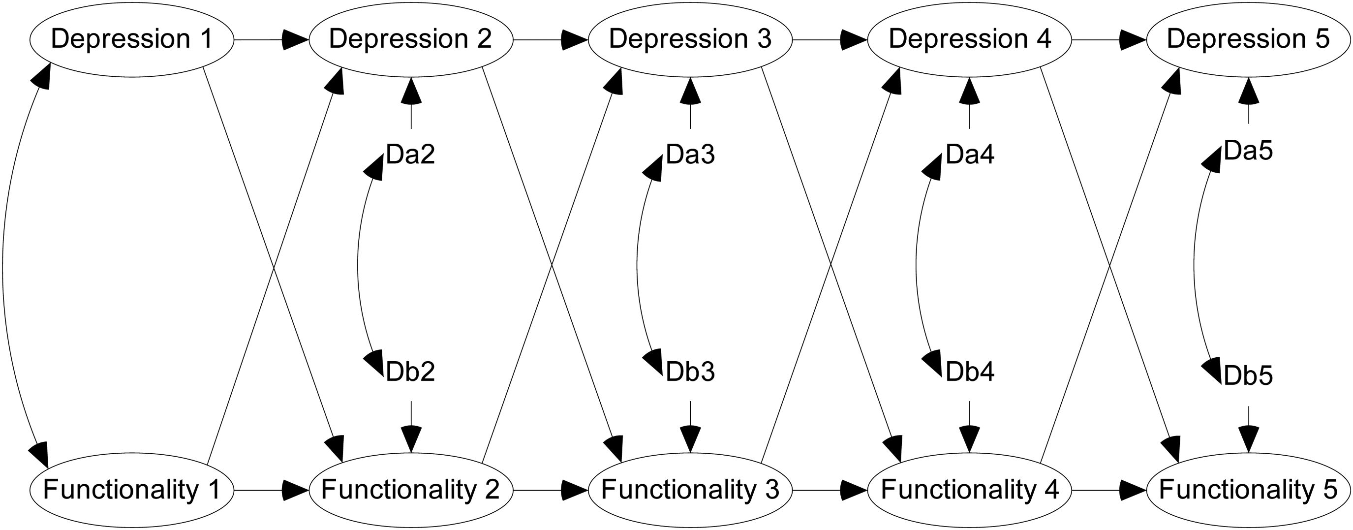
Bivariate autoregressive cross-lagged model.

Regarding the current example, understanding the causal relationship between depression and physical functioning has been an important issue in gerontological and health care research. The first step is to place both of the previously tested univariate models of depression and physical functioning into a bivariate autoregressive model correlating the disturbances (e.g., Da2 and Db2) between variables within the same wave. The second step is to add the cross-lags from the immediately previous time period of depression to the immediately next time period of physical functioning as well as from the immediately previous time period of physical functioning to the immediately next time period of depression. For example, when examining waves 2 and 3, depression at time 2 is cross-lagged on to physical functioning at time 3, while physical functioning at time 2 is cross-lagged on to depression at time 3. Additionally, the autoregressive paths for depression at time 2 going to depression at time 3 and from physical functioning at time 2 to physical functioning at time 3 must be present to test for causal ordering. The autoregressive paths must also be present to identify if the cross-lags from one variable (e.g., depression at time 2) to the next wave variable (e.g., physical functioning at time 3) predict anything above and beyond that which is predicted by the autoregressive path of time 2 physical functioning to time 3 physical functioning.

A special form of the bivariate autoregressive model is known as the bivariate autoregressive contemporaneous model. The autoregressive cross-lagged model relies on controlling two variables at the immediate prior time period (autoregressive coefficients) to identify the strength of the standardized cross-lag coefficients from one time period to the next. The difference is that while the contemporaneous model also controls two variables at the immediate prior time period (autoregressive coefficients), it identifies causal ordering of the two variables (e.g., depression and physical functioning) within the same wave based on the strength of the standardized contemporaneous coefficients. The advantage of this model is that causality can be tested within the same time wave as the phenomena are happening when compared to cross-lagged models that test causality across two time waves. Figure 3 shows the path diagram of the bivariate autoregressive contemporaneous model for the relationship between depression and physical functioning.

OPEN IN VIEWER

Figure 3.

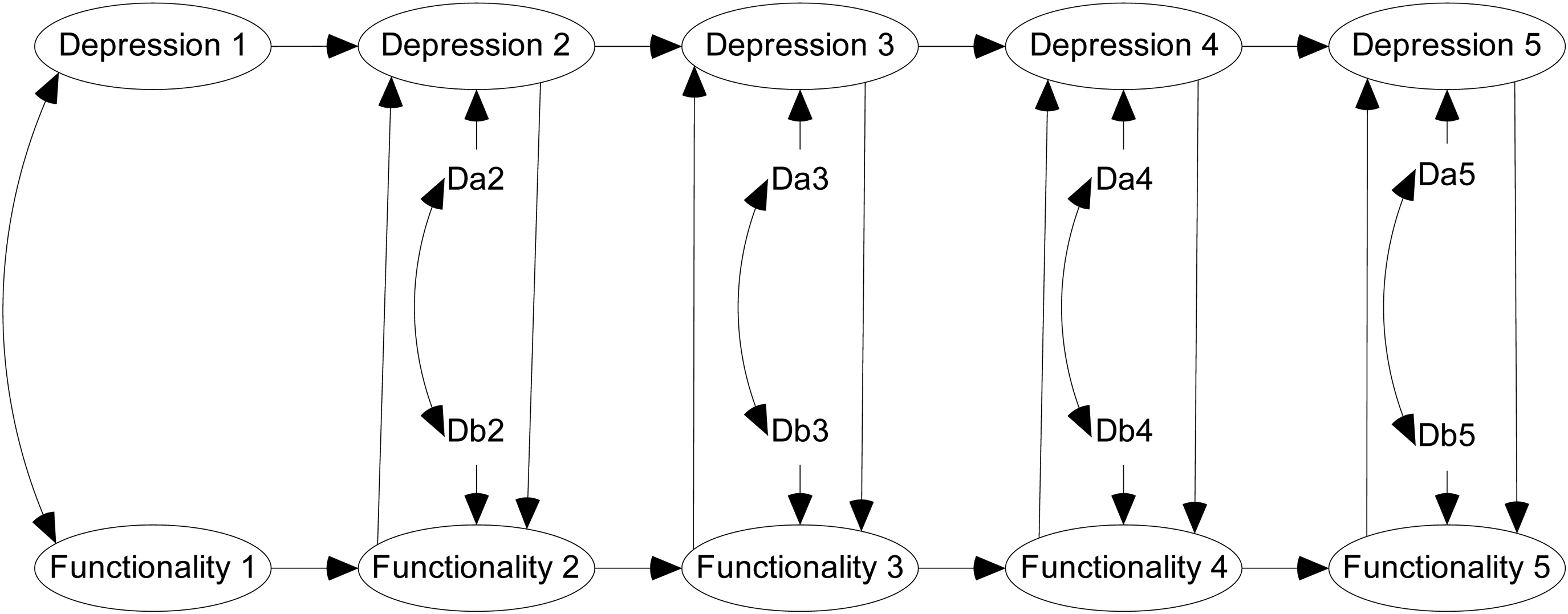
Bivariate autoregressive contemporaneous model.

In testing the bivariate autoregressive contemporaneous model, the same first step is used as used in testing the cross-lagged model. Both of the previously tested simplex univariate models of depression and physical functioning were placed into a bivariate autoregressive model correlating the disturbances (e.g., Da2 and Db2) between variables within the same wave. The second step is to add the contemporaneous paths from depression to physical functioning within the same wave as well as from physical functioning to depression within the same wave. For example, when examining wave 3, depression at time 3 predicts physical functioning at time 3, while physical functioning at time 3 predicts depression at time 3. Additionally, the autoregressive paths for depression at time 2 going to depression at time 3 and from physical functioning at time 2 to physical functioning at time 3 must be present to test for causal ordering. The autoregressive paths must be present to identify if the contemporaneous path from one variable (e.g., depression at time 2) to the next variable (e.g., physical functioning at time 2) within the same wave predict anything above and beyond that which is predicted by the autoregressive path of time 2 physical functioning to time 3 physical functioning. Conversely, the contemporaneous path from physical functioning at time 2 to depression at time 2 can also be tested.

Summary

Bivariate autoregressive models are extremely useful for identifying causal ordering between two variables in longitudinal analyses. The purpose of this paper was to introduce the concept of autoregressive models and the steps needed to test and develop bivariate autoregressive and cross-lagged models and bivariate autoregressive contemporaneous models. This paper emphasized the importance of developing solid univariate simplex models that could be combined into bivariate models to test for causal ordering. Two different bivariate approaches were also introduced for testing causal ordering. Both cross-lagged and contemporaneous models can be used to identify causality. Autoregressive models are a useful tool for gerontological research using longitudinal analyses, and it allows researchers to gain a better understanding of how two or more variables interrelate to each other over time. While a useful tool to explore the intricacies of the interplay among variables over time, surprisingly, it is a technique that has been used on a limited basis in gerontological research.