
Abstract
The purpose of this research note is to introduce a latent growth curve reconstruction approach based on the Tabu search algorithm. The approach algorithmically enables researchers to optimally determine at both the individual and the group levels the order of the polynomial needed to represent the latent growth curve model. The procedure is illustrated using empirical data along with an easy to use computerized implementation.
The accurate modeling of longitudinal data to reveal individual differences is a key component for understanding developmental change within the social and behavioral sciences. Numerous statistical models to depict longitudinal data at the individual and group levels have to date been proposed and detailed descriptions of them can be found in the literature (e.g., Bollen & Curran, 2006; Flora, 2008; Grimm & Marcoulides, 2016; Grimm et al., 2016; Little, 2013; Marcoulides, 2018; Marcoulides & Khojasteh, 2018; McArdle & Nesselroade, 2014). Because these various statistical models generally involve the construction of a mathematical function best fitting a set of data points, they are also often characterized as curve reconstruction techniques (Rusdi & Yahya, 2014).
One particularly informative and popular curve reconstruction technique used to examine intraindividual changes, interindividual differences in intraindividual changes, as well as a variety of other intra- and interindividual disparities is latent growth curve modeling (Baltes & Nesselroade, 1979). A strategy that is frequently used in this approach to characterize longitudinal data is to model the growth trajectories as linear functions. While linear patterns of change are regularly encountered in longitudinal social and behavioral science research, nonlinear patterns are also quite prevalent (Grimm et al., 2016). Consequently, latent growth modeling is frequently conducted in a confirmatory modeling manner where specific hypothesized mathematical functions are tested against the longitudinal data to determine which among different patterns of change (e.g., linear, quadratic, exponential, etc.) best represents the intra- and interindividual changes and their differences over time (Bollen & Curran, 2006; Grimm & Marcoulides, 2016; Grimm et al., 2016). Although this confirmatory modeling convention is widely adopted, relying exclusively on this approach can limit a researcher’s insight into different possible patterns of growth as each hypothetical model must be a priori explicitly specified (Bollen & Curran, 2006; Grimm et al., 2013). For this reason, exploratory models that feature limited prespecified characteristics have been suggested for determining the patterns of growth (Grimm et al., 2013; Marcoulides, 2018). These models are particularly useful because the exploration builds knowledge based almost exclusively on the examined data, which is the reason they are also sometimes called machine learning algorithmic models or unsupervised data mining models (Marcoulides & Falk, 2018).
Due to a variety of complexities that can be encountered when fitting exploratory latent growth curve models, to date many different approaches have been proposed in the literature for this purpose. For example, Grimm et al. (2013) introduced a direct extension of so-called Tuckerized curves (Tucker, 1958, 1966) as an exploratory way to model change processes based on a principal components analysis with explicit constraints. A somewhat similar method for exploring growth models based on the use of principal component analysis was also proposed by Davison (2008) and by Timmerman (2004). Although these researchers all demonstrated the benefits of using these models for exploratory purposes, some major limitations with the approaches include the need to constrain an unspecified subset of values to equal 0 or some other value, determining the most appropriate manner to decide on the solution structure and its rotation and determining the number of principal components to take into account (Davison, 2008; Grimm et al., 2013; Timmerman, 2004).
Another exploratory approach recently introduced by Bentler (2018) is based on evaluating via a regression analysis the order of the polynomial function to describe growth, where the actual order of the polynomial function can in principle be as high as the order of the number of repeated measurement occasions (Bentler, 2018; Bollen & Curran, 2006). Although this proposed approach can be readily applied to select from intercept, slope, quadratic, cubic, quartic, or higher-order model trends, its reliance on a hierarchical regression analysis strategy can limit its ability to yield the best solution and to differentiate among models with more complex patterns of change (Hocking, 1976). Thompson (1995) described this concern as “a linear series of conditional decisions not unlike the choices one makes in a maze. An early mistake in the sequence will corrupt the remaining choices (p. 532).” This is because the values of the parameter estimates and the obtained significance levels of each model can change as a function of when they were entered into the model and what other aspects of the model are present. Another limitation with this proposed exploratory approach is that it does not take into account individual differences and instead focuses only on information about group means and mean curves (Bentler, 2018).
The purpose of this research note is to introduce a simple extension to the original curve reconstruction method proposed by Bentler (2018). The suggested approach overcomes the abovementioned limitations and algorithmically enables researchers to optimally determine the order of the polynomial in the growth curve model. The approach can also be used to simultaneously uncover both individual and group level growth estimates. The approach uses Tabu search (TS) strategies to accomplish the task of curve reconstruction. TS was originally introduced for solving a variety of complex optimization problems and has over the years effectively been used for many other problems within the structural equation modeling framework (e.g., specification searches, the creation of short forms, determining the location of knots in spline models; Marcoulides, 2018; Marcoulides & Falk, 2018; Raborn et al., in press). Here a modified version of the original TS approach is introduced and integrated into the exploratory latent growth curve model fitting process and facilitated by a common structural equation modeling framework. The proposed approach effortlessly makes it possible for a researcher to determine directly from the data the functional form of the trend over time at both the individual and group levels.
The remainder of the article is organized in the following way. First, the general conceptual ideas behind model selection via TS are briefly reviewed. These are then demonstrated by working through an empirical example. Finally, a computerized implementation of the approach via the widely used and freely available statistical programming language R is discussed.
Overview of TS
The main idea behind the TS approach is to continually adjust a currently selected solution by examining other potential results in the neighborhood of that solution. If an examined neighboring result is found to fit better than the currently determined solution, it is then selected as the new best solution. If not, the examined neighboring result is basically marked as “tabu.” In other words, the result is placed on a forbidden list, so that it is not reconsidered. Once a solution is examined and stored, it thereon acquires an off-limits status. It is because of this off-limits status that the approach was labelled Tabu, utilizing the alternative English spelling of the word taboo (Hansen, 1986; Marcoulides et al., 1998).
To implement the TS approach, the following key features are necessary 1 : (i) a starting model, (ii) a neighborhood definition, (iii) a model selection criterion, (iv) a list of models examined, and (v) a stopping criterion. Each of these aspects is briefly described next. A flowchart outlining the process is provided in Figure 1.
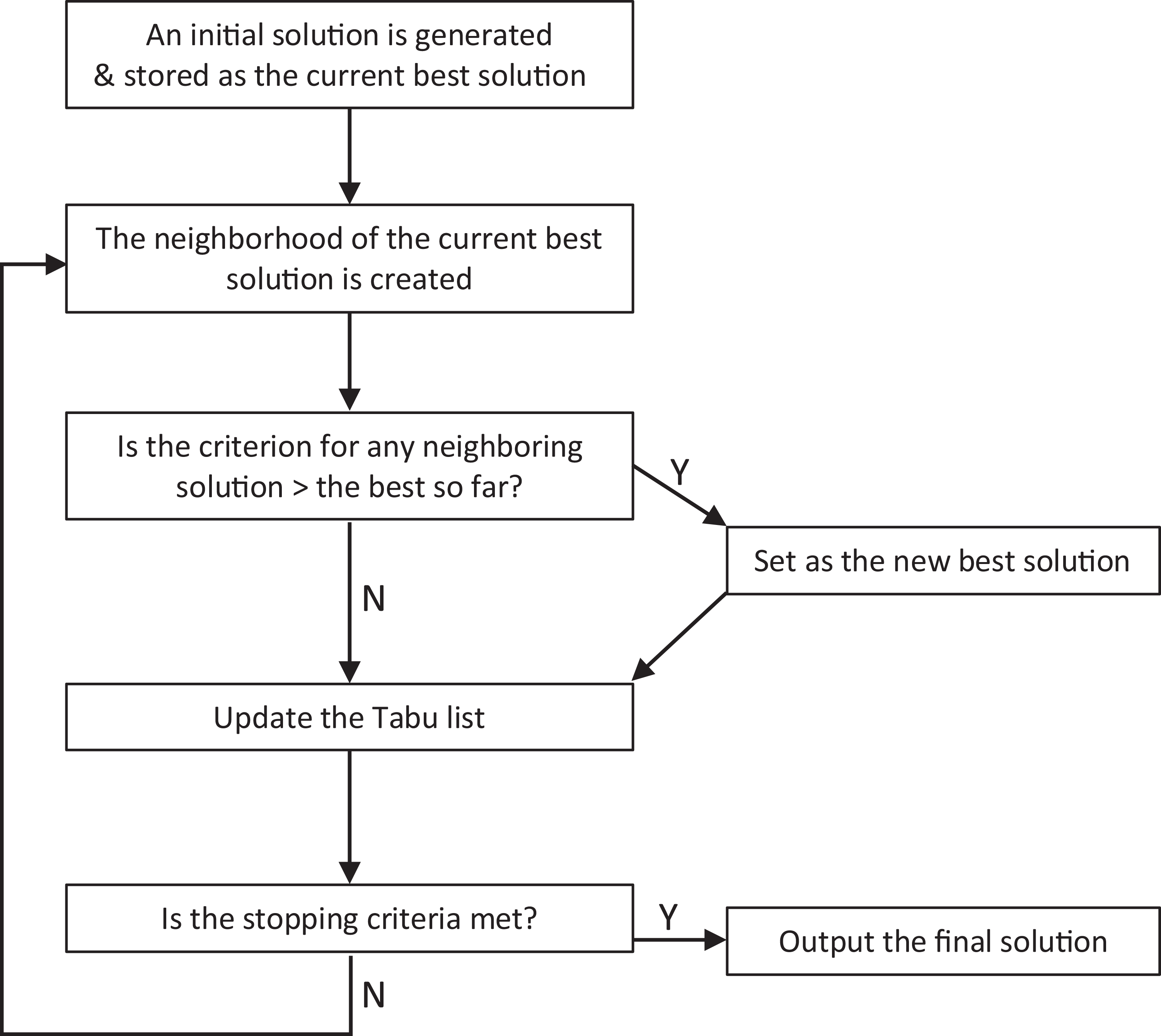
Flowchart of the Tabu Search Algorithm.
A Starting Model
Any user-defined growth function (linear, quadratic, cubic, etc.) can be selected to serve as the starting model. Considering that the actual order of the polynomial function can be in principle as high as the order of the number of measured time points, in this implementation the algorithm begins by randomly selecting the order of the polynomial function and using that as the starting model. This designated starting model provides an initial solution for the search to then proceed through its iterations. The TS approach permits the implementation of any and all types of constraints on the parameters of the model, thus any number of strategies that institute model searches under particular constraints can be accommodated. Accordingly, if a researcher wishes, based on theoretical grounds, to attend only to positive, even-numbered, or odd-numbered polynomial orders, the TS approach can be augmented to include this information. A common taxonomy that is applied to describe these activities borrowed from the field of data mining refers to them as “supervised,” “semi-supervised,” or “unsupervised” (Marcoulides & Falk, 2018). Supervised activities are guided entirely with prior knowledge, while unsupervised activities are entirely data driven. Semi-supervised activities start off with some supervised information but proceed with an unsupervised exploration of the data. Given the demonstrated excellent convergence of the TS approach (Glover & Hanafi, 2002; Glover & Laguna, 1993), the analyses presented in this article did not restrict the search for determining the best admissible solutions to specific supervised model situations and began an unsupervised search with a random start model. Any alternative choices could, however, be easily incorporated into the proposed TS growth reconstruction approach.
A Neighborhood Definition
The neighborhood definition applied in this implementation is one in which all feasible subsets of a current solution (beginning with the starting solution) are enumerated by including one additional variable into the model, one less variable, or replacing variables in the model by one not in the model. For example, in a regression analysis with k = 5 variables
Diverse definitions of the neighborhood can be used to conduct a TS, with each potentially affecting the efficiency and accuracy of the solution. For example, in the above case with k = 5 variables if a researcher decided to only add or remove variables, this would immediately reduce the size of the neighborhood and expedite convergence time. However, if the newly defined neighborhood is too small, it could jeopardize the accuracy of the final solution. This implies that if the neighborhood structure is inadequate, the TS approach will most likely not be successful. Currently, the most popular neighborhood definition approach (and the one used in the proposed reconstruction method) is based on the notion of defining and then dynamically examining the entire neighborhood of the parameter space under consideration. Characterized in this manner, the TS approach may be viewed as a dynamic neighborhood method, whereupon the neighborhood can change according to the history of the search (Glover & Laguna, 1993). Other strategies that are gaining popularity involve adopting a variable (random) neighborhood selection approach, as in the recently proposed hybrid TS algorithm (Marcoulides, 2018). It has been suggested that this hybrid approach “may reduce convergence time while increasing the dispersion of the search over the entire solution set” (Raborn et al., in press, p. 17). However, additional research is needed to examine the precision and convergence times of this new hybrid algorithm.
Model Selection Criterion
Different criteria can be used to evaluate a model in TS. In this implementation, model selection is based on an evaluation of the computed model R 2, the F-statistic based on the obtained R 2, and the statistical significance of the corresponding F-statistic (Abramowitz & Stegun, 1968). The model yielding the lowest significance level and largest R 2 among all possible model subsets is correspondingly selected. As past research has shown that the choice of fit criterion in TS does not generally impact the identification of the correct model, any other model selection criterion would be expected to provide similar results to those reported here (Marcoulides & Leite, 2014).
List of Models Examined
The list containing a record of models examined is called the Tabu list and its maximum length is called the Tabu size. Until a new best model is found, the last entry in the Tabu list is discarded whenever the Tabu size is exceeded. In the event a new best model is found, then the entire Tabu list is emptied and the search begins again but with the new best model now acting as the starting solution. Standard Tabu lists that are able to explore the solution near the optimum are most commonly implemented as lists that are fixed and of limited length (Glover & Lacuna, 1993). In this implementation, the Tabu size was set at 10 (following recommendations provided by Drezner & Marcoulides, 2009 and verified by Raborn et al., in press).
Stopping Criterion
The stopping criterion in TS is equivalent to the number of iterations that the algorithm must perform without improving the best-so-far solution. A number of stopping criteria can be adopted for this purpose. These include (i) simply stopping the search after a fixed number of iterations, (ii) stopping the search after some specific number of consecutive iterations occur without an improvement in the solution, (iii) stopping the search when the objective value itself reaches a prespecified threshold value (assuming of course that this threshold value is somehow known), or (iv) stopping the search after a fixed amount of computer CPU time is reached. The stopping criterion in this implementation was set at 30 iterations without improving the best-so-far solution (Marcoulides, 2018).
Latent Growth Model Specification
Consider a longitudinal study comprised of a set of t consecutive measurements for a variable y obtained from a sample, with the t measurement times being either equally or unequally spaced and, for simplicity, assume that there are no relevant explanatory covariates (although the model can easily be extended to include covariates). Assuming a mean vector μ and the covariance matrix Σ of the repeated measures are a function of factor loadings Λ, latent variable means η i, a latent variance–covariance matrix Ψ, and a residual variance–covariance matrix Θ (e.g., Raykov & Marcoulides, 2006), a latent growth curve model can be specified as a confirmatory factor model with a mean structure as follows:


If a linear growth model is specified so that the reference point is the initial status of the variable y, the Λ factor-loading matrix (in the case of seven time points) is
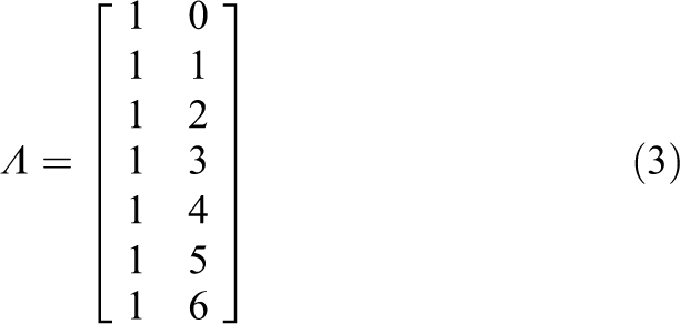
The first column of Λ expresses the fixed factor loadings for the intercept factor and the second column expresses the fixed factor loadings for the linear slope factor. Thus, in the above linear growth equation, the factor loadings for the intercept factor
If a quadratic growth model is instead specified, then the Λ factor-loading matrix is expanded to the following structure:
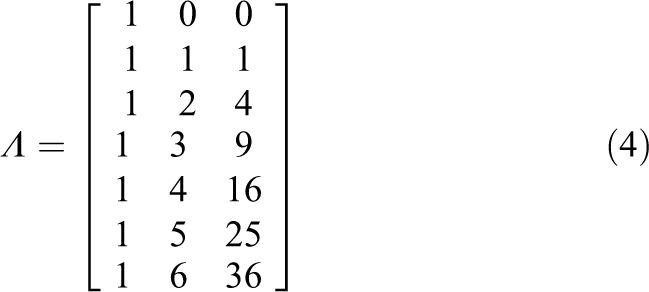
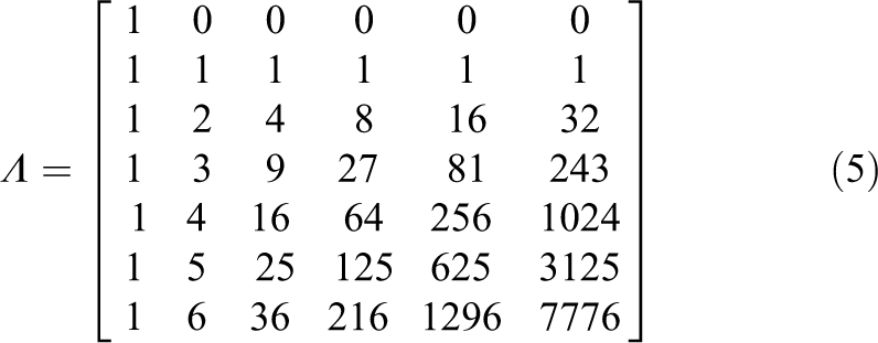
The first column of Λ again expresses the fixed factor loadings for the intercept factor and the second column expresses the fixed factor loadings for the linear factor, while the third column now expresses the fixed factor loadings for the quadratic factor. Thus, the number of factors in the matrix Λ in essence determines the diverse order of the polynomial that can be used to describe the growth over time, whereupon the actual order of the polynomial can in principle be as high as the order of the number of repeated measurement occasions (Bollen & Curran, 2006). For example, for a complex quintic (fifth order) growth model, the Λ factor-loading matrix is specified as follows:
Given the complexity of the potential number of factors in the matrix Λ, the difficulty is then to determine the appropriate order of the polynomial of the function needed to represent well the observed growth trajectories. The proposed TS approach provides an algorithmic way to optimally select in an exploratory manner the appropriate number of factors to use in the Λ factor-loading matrix for the analysis of longitudinal data but is still based on the latent growth modeling framework. Accordingly, the proposed approach does not require a researcher to make a decision concerning the selection of the appropriate number of factors as this is determined automatically and directly from the examined data. It is advocated that having access to such a new approach overcomes concerns that have been raised with existing exploratory growth mixture modeling approaches by automating the entire selection process.
It is important to note that although the proposed growth reconstruction approach is demonstrated using polynomial curves, many other functional forms could also be easily incorporated into the TS and examined in the same manner. For example, a multitude of different nonlinear curve shape forms (e.g., Bleasdale–Nelder curves, cosine, cyclical sine; exponential, Gompertz, hyperbolic, Janoschek curves, logarithmic, logistic, Michaelis–Menten curves, monomolecular, Morgan–Mercer–Flodin curves, poly-ratio, Richards curves, Weibull curves, or von Bertalanffy curves; Goldstein, 1979; Little, 2013) could easily and similarly be parameterized into the presented TS algorithm. This is because past research (e.g., Browne & du Toit, 1991; du Toit & Cudeck, 2001; Grimm et al., 2010) has shown that all these other functional forms can in fact be encoded in different ways as elements of the design factor-loading matrix Λ and then directly estimated using higher-order polynomials. As such, as long as the elements of the design factor-loading matrix Λ can be specified, the optimization search can be conducted and applied for the construction and fitting of any growth curve or combination of curves.
A number of researchers have also suggested the use of orthogonalizing approaches to ensure the stability of computed values, especially in models with powered terms (e.g., Little et al., 2006) 2 . Orthogonal polynomial contrasts essentially involve a series of constraints on terms within the design factor-loading matrix Λ similar to the different nonlinear curve shape forms described above. Alternatively, the TS algorithm could even be expanded to include the estimation and comparison of values based on both orthogonal and non-orthogonal polynomial terms simultaneously. To simplify the description of the reconstruction approach illustrated in this article, orthogonal polynomial contrasts were not implemented in this study. However, these could most certainly be readily applied in a similar manner as many other functional forms could also be incorporated into the TS approach. Thus, the reconstruction approach proposed in this article focused mainly on common polynomial curves with the understanding that these could be readily extended to allow for a wide series of flexible and interesting growth models.
Illustrative Example
This section demonstrates the application of the proposed TS algorithm for determining, in an exploratory manner and directly from the data, the functional form of the trend over time at both the individual and group levels. The illustration utilizes empirical longitudinal data first reported by Pan and Fang (2002) in Table A.1 (p. 353—Online Appendix Data Sets). The original study focused on the measurement of weight in pounds of 13 male mice measured 7 times at intervals of 3 days from birth to weaning. 3 The same empirical study was also examined by Bentler (2018). Figure 2 displays the growth curves for this illustrative sample across the seven consecutive time points and indicates that the trajectories clearly follow a pattern characterized by nonlinear growth in the measured weight variable. Based on these data, Pan and Fang (2002) reported that the average growth curve was best represented by a quadratic growth trajectory, a conclusion that was also endorsed using the curve reconstruction method proposed by Bentler (2018).
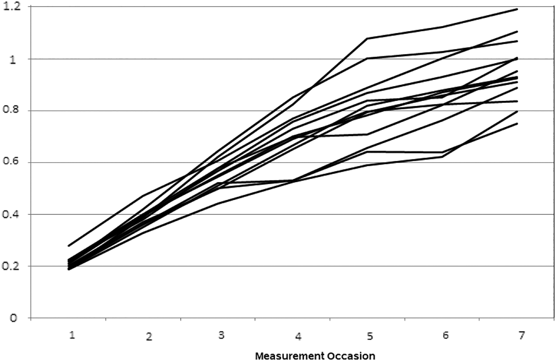
Growth Trajectory Plot of Each Observation in the Illustrative Data.
Imagine that we have been presented with this longitudinal data set and wish to perform an analysis to determine which among different possible patterns of change best represent the observed growth trajectories (in this specific case among either linear, quadratic, cubic, quartic, quintic, or sextic pattern, corresponding from an intercept only model to a sixth order model, respectively). To perform this activity, the proposed TS algorithm implemented in the publically available software program R (R Core Team, 2018) is applied to this data set (the necessary R code is provided in Online Appendix A). The input required to perform the analyses for the TS algorithm includes the matrix Λ and the observed data matrix 4 .
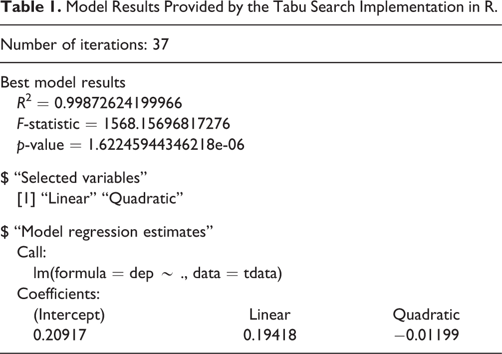
Upon running the provided R code, the results generated by the proposed algorithm are readily determined. For example, using the observed mean values for the seven ordered time points {0.211, 0.386, 0.551, 0.686, 0.805, 0.862, and 0.950, respectively} and the specified Λ matrix in equation (5), the results displayed in Table 1 would be obtained. These results indicate that the average growth curve is best characterized by a quadratic growth model, with estimated factor mean values of 0.209, 0.194, and −0.012 for the Intercept, Linear, and Quadratic factors, respectively, and with R 2 = 0.9987, F-statistic = 1568.16, and p-value = 1.62 × 10⁻⁶. These results concerning the observed means were of course expected, given the findings reported by both Pan and Fang (2002) and by Bentler (2018). However, upon examining further via the TS approach the individual observations in the illustrative data set, some important insights concerning the different patterns of growth become evident. Specifically, when the proposed TS approach is applied to the observed scores for each of the 13 observations, the summarized results displayed in Table 2 are obtained. These results reveal that the polynomial order of the models selected for each observation in fact varies from linear (first order) to quintic (fifth order). Specifically, there are four observations that are best represented by a first-order polynomial (a linear model), two observations a second-order polynomial (a quadratic model), three observations a third-order polynomial (a cubic model), two observations a fourth-order polynomial (a quartic model), and two a fifth-order polynomial (a quintic model). Thus, by applying the TS algorithm to these empirical data, it is evident that more complex trajectory patterns were revealed and better characterized the different nonlinear changes occurring in the measured weight as the mice got older. The detection of these types of nonlinear changes highlights the benefit of the proposed approach in algorithmically determining the polynomial order of the growth patterns at both the observation and the group levels. It can even provide researchers with an effective tool to discern potential differences between the examined observations and help identify those that belong together in a cluster based solely on their computed growth functions.
Model Results Provided by the Tabu Search Implementation in R.
Summary of Modeling Results for All 13 Observations Provided by Tabu Search.
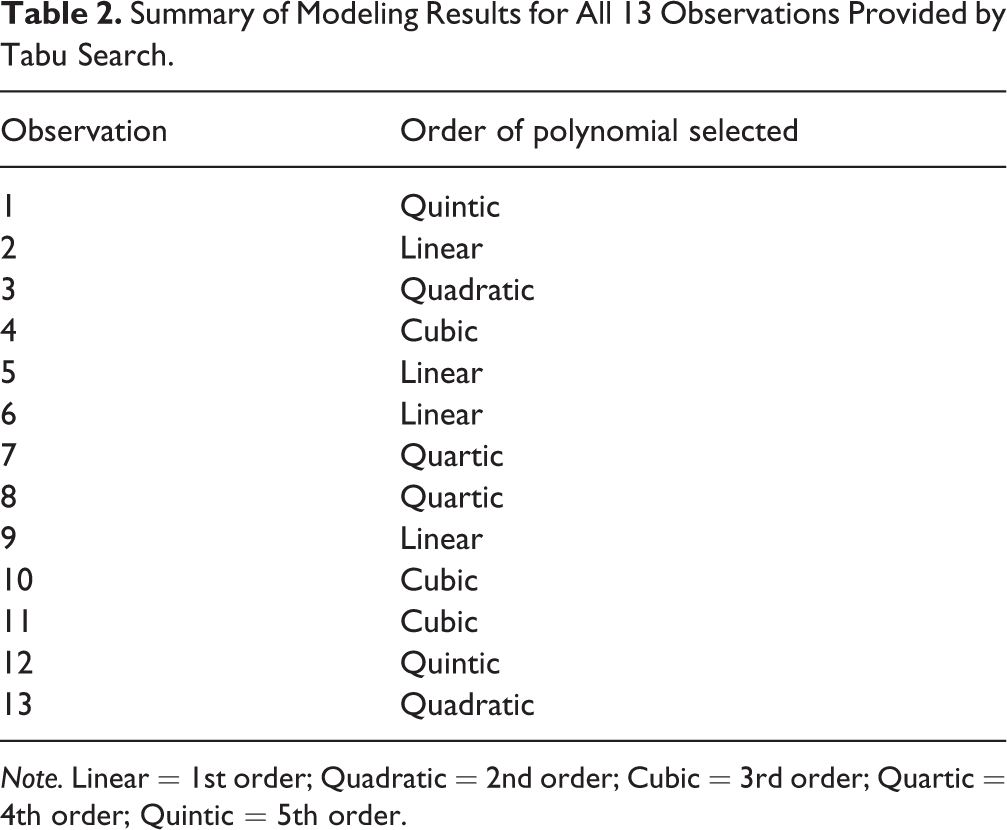
Note. Linear = 1st order; Quadratic = 2nd order; Cubic = 3rd order; Quartic = 4th order; Quintic = 5th order.
Concluding Remarks
This research note introduced TS as a curve reconstruction approach that can help researchers examine patterns of growth trajectories in longitudinal data analyses. The approach algorithmically determines via an all-possible-subset-regression type analysis the order of the polynomial function needed to describe the latent growth model. The approach is especially applicable for studying in an exploratory manner developmental processes where complex patterns of growth may be present. The procedure was illustrated using empirical data obtained from a simple longitudinal study and demonstrated the invaluable capabilities of the procedure for automating the entire process of fitting latent growth curve models.
The proposed approach is ideally suited for fitting data in settings where confirmatory modeling strategies involving specific hypothesized mathematical functions corresponding to different patterns of change might not be appropriate. By essentially utilizing what some researcher have referred to as a “bottom-up-approach” in which data are analyzed person by person, more insightful comparisons between the dynamics of different individuals could also be achieved (Hamaker et al., 2018). The method can also be used irrespective of the frequency of data collection or the complexity of the individual growth patterns and provides an alternative lens through which longitudinal processes can be examined. Many options are available for the modeling of data from longitudinal studies and the approach introduced here represents a method to entirely automate the determination of patterns of individual and group growth trajectories. It is hoped that researchers will apply the proposed procedure to a variety of longitudinal studies across different disciplines to accurately capture any complex growth patterns that might be encountered.
Supplemental Material
Supplemental Material, JBD941170_Appendix_A - Latent growth curve model selection with Tabu search
Supplemental Material, JBD941170_Appendix_A for Latent growth curve model selection with Tabu search by Katerina M. Marcoulides in International Journal of Behavioral Development
Footnotes
References
Supplementary Material
Please find the following supplemental material available below.
For Open Access articles published under a Creative Commons License, all supplemental material carries the same license as the article it is associated with.
For non-Open Access articles published, all supplemental material carries a non-exclusive license, and permission requests for re-use of supplemental material or any part of supplemental material shall be sent directly to the copyright owner as specified in the copyright notice associated with the article.