




Abstract
Landmarks are ideal wayfinding tools to guide a person from A to B as they allow fast reasoning and efficient communication. However, very few path-finding algorithms start from the availability of landmarks to generate a path. In this paper, which focuses on indoor wayfinding, a landmark-based path-finding algorithm is presented in which the endpoint partition is proposed as spatial model of the environment. In this model, the indoor environment is divided into convex sub-shapes, called e-spaces, that are stable with respect to the visual information provided by a person’s surroundings (e.g. walls, landmarks). The algorithm itself implements a breadth-first search on a graph in which mutually visible e-spaces suited for wayfinding are connected. The results of a case study, in which the calculated paths were compared with their corresponding shortest paths, show that the proposed algorithm is a valuable alternative for Dijkstra’s shortest path algorithm. It is able to calculate a path with a minimal amount of actions that are linked to landmarks, while the path length increase is comparable to the increase observed when applying other path algorithms that adhere to natural wayfinding behaviour. However, the practicability of the proposed algorithm is highly dependent on the availability of landmarks and on the spatial configuration of the building.
Introduction
Similar to outdoors, the complexity of a building can force a navigator to rely on route instructions. If these directions are formulated by another person, chances are that features of the environment are integrated to clarify the instructions. This brings us to a major principle with respect to giving directions, namely referring to landmarks (Richter and Duckham, 2008). These salient geographic elements structure a human’s mental representation of space (Richter and Winter, 2014), which is central in our ability to navigate as it represents all known spatial relations between objects and spaces and enables us to define routes and to describe our location (Iaria and Barton, 2010). The prime function of landmarks is to specify locations. They define a place. However, while a place exhibits a high level of information and details, a landmark is an anchor point that is abstracted to a node without internal structure. In this way, the representational complexity is reduced. Consequently, landmarks are ideal wayfinding tools for directing a person from A to B as they allow fast reasoning and efficient communication (Richter and Winter, 2014). Moreover, the use of landmarks is often linked with the quality of route instructions as they are related to the natural cognitive navigation process of humans (Lovelace et al., 1999).
Within this context, this article focuses on landmark-based path-finding indoors whereby a route between an origin and a destination is selected based on the availability of landmarks. More than a decade ago, Caduff and Timpf (2002) addressed the fact that landmarks were mostly used to enrich existing (shortest) paths and rarely formed the basis of indoor routing algorithms. Not much has changed since then. Apart from problems related to landmark identification, this stems from the difficulty to model the indoor environment. Therefore, the main objective of this article is to present a new approach of landmark-based path-finding that is based on an existing convex partition of indoor space called the endpoint partition, which was developed by Peponis et al. (1997). Following, this article wishes to verify whether this approach to reduce the path complexity leads to useful paths with a reasonable path length.
The article proceeds by defining landmark-based path-finding and presenting existing indoor approaches. Following, the endpoint partition, its properties and selection as spatial model are explained. Next, the algorithm used to construct and implement the routing graph is presented. Finally, the usability of the proposed approach is discussed on the basis of an empirical comparison between e-paths and shortest paths.
Landmark-based path-finding
Basiri et al. (2013) stated that landmark-based path-finding is determining ‘a path which traverses a shorter distance to get to the destination but passing more landmarks on the way’ in order to provide a more reliable path that is easier to follow. However, Duckham and Kulik (2003) argued that the simplest path, with respect to the cognitive load it causes, should not take distance into account as a path selection criterion because navigators are prepared to follow longer routes if these are easier to follow. Following, maximising the number of landmarks along a path is not necessarily beneficial as this increases the possibility that more identical or very similar objects are present, especially in an indoor environment where there is less variety in terms of type and number of distinctive landmarks. These ‘false landmarks’ mislead the navigator as they may be erroneously linked to certain wayfinding actions. This renders the path less reliable and the landmarks less informative (Elias, 2003; Stankiewicz and Kalia, 2007). Furthermore, in a building most directions are given in advance and, as a consequence, have to be remembered during the navigational task, because there are no or very limited positioning systems that can deliver adaptive path calculations comparable to commonly used outdoor navigation devices. In this case, one must memorise the directions by constructing a cognitive representation of the path (Mast and Wolter, 2013). By keeping the number of wayfinding actions (and the amount of landmarks linked to them) to a minimum, the cognitive cost can be reduced (Elias and Sester, 2006). This is similar to the simplest path algorithm whereby the overall complexity of the path is minimised (Duckham and Kulik, 2003). A simplest path is calculated based on weights attributed to each (type of) intersection. These weights reflect the complexity of the information needed to explain the wayfinding action that should take place at that intersection. In order to minimise the overall weight of a path, the simplest path algorithm selects ‘simpler’ intersections and/or reduces the number of intersections. However, the simplest path will not always select the path with a minimum of intersections as this may require complex intersections which could increase the overall weight of the path. In contrast, the presented landmark-based path-finding algorithm makes no differentiation between intersections and minimises the number of wayfinding actions or turns (at intersections). In addition, these actions must be linked to landmarks. For these reasons, another definition of landmark-based path-finding is used within the scope of this article, namely determining a path from a starting point to a destination that can be explained by a minimum of actions linked to landmarks to reduce the cognitive load of users. Note that landmark-based path-finding is different from landmark-based navigation in which the instructions of an existing path (e.g. shortest path) are enriched with landmarks to increase the instructional quality of that path in support of the coordinated movement in an environment.
Even though several studies have pointed out that referring to landmarks is inherent to natural wayfinding behaviour, very few have integrated landmarks in the path generating process indoors. In 2002, Caduff and Timpf presented a theoretical framework for landmark-based path-finding called the ‘landmark spider’. Here, the clearest path was found by implementing weights attributed to the saliency of point-like landmarks and their position with respect to the observer (i.e. distance and orientation) in a revised Dijkstra’s path algorithm. Although the landmark spider was developed with an outdoor environment in mind, it is applicable indoors as well. Ten years later, Heiniz et al. (2012) proposed an indoor landmark-based navigation system that calculates the shortest route by using Dijkstra’s shortest path algorithm based on a graph in which the nodes represent logical areas that comprise a set of unique attributes or landmarks visible from this point. These nodes can function as waypoints that connect each route segment of the selected path. As a result, a set of landmarks is available as reference at each start and endpoint of a route segment.
In both studies, however, it is unclear how the building’s spatial structure was modelled and how the available landmarks or reference points were linked to the graph. Caduff and Timpf (2002) only mention the use of a route network. Heiniz et al. (2012) divided the building into logical areas or waypoints that contain a set of landmarks visible from the user’s point of view. They do not mention how large rooms are subdivided into these logical areas, how the spatial model incorporates or deals with obstacles (e.g. pillars) that obstruct the view on the mentioned reference points and how different paths within larger areas are defined. The last mentioned aspect is important as pedestrians, who are characterised with a high degree of freedom in movement, often come across open areas where there are no distinct paths or decision points (i.e. scene space) (Mast and Wolter, 2013). In addition, rooms can strongly vary in size, shape and level of connectivity. For these reasons, an adequate spatial model of the indoor environment needs to be selected. In this study, the endpoint partition, which was drawn up by Peponis et al. (1997), is implemented.
Endpoint partition
As the modelling of indoor spaces has been the subject of numerous studies arising from various points of view or goals, this article does not aim to add to this broad range of indoor models. Instead an existing spatial model was selected that supports the practical functionalities of landmarks.
First, landmarks are traditionally seen as part of view-action pairs. Here, landmarks serve as associative cues for basic motor activities (e.g. ‘at the statue, take a left turn’) (Lovelace et al., 1999; Mast and Wolter, 2013; Montello, 1998). Associative cues are also called pointers as they send a navigator away from a specific location. To support this use of a landmark, distinct subareas in a room in which one can refer to this feature associatively must be defined. Furthermore, the landmark linked to this subarea must be visible from all possible positions within this subarea. As such, rooms must be modelled as a collection of convex subspaces. The decomposition of indoor space into a (minimal) set of convex sub-regions forms the basis of various spatial models. In these cases, however, this is done starting from the notion that the spatial structure of a building imposes constraints upon movement in order to draw more realistic paths that do not cross walls or obstacles. Although this is correct, within the context of landmark-based path-finding, the subdivision of space should also represent the structural features and changes of the building’s layout as these features influence the construction and use of the cognitive map. This is more in line with the concept that landmark-based path-finding is based on continuously comparing the cognitive map with reality whereby salient elements act as points of correspondence (Heiniz et al., 2012; Presson and Montello, 1988).
In addition, landmarks can serve as beacons. Here, landmarks are used simply in terms of approaching (or avoiding) them. In this way, a chain of landmarks or locations is visited in order to reach the final goal location. This use of landmarks is linked to the most basic level of navigation strategy (i.e. guidance) (Wang et al., 2014). In contrast to an associative cue-based path, no additional information (i.e. the appropriate action) needs to be encoded and the navigator can focus completely on the landmark identity, which is easier to remember (Waller and Lippa, 2007). In order to guide a person towards a beacon, one must be able to see the beacon and to move directly towards it. Therefore, the subspacing must take into account walls, obstacles and non-navigable areas to determine the visibility and accessibility of a landmark along the line of sight.
Space syntax measures focus on the spatial structure of a building and the visibility within that building. Additionally, these measures are linked to wayfinding behaviour (Hölscher et al., 2012). Within this context, the endpoint partition sees to these requirements and enables the representation of indoor space by a set of non-overlapping cells whereby each cell is characterised by semantics, geometry and topology (OGC, 2014). The endpoint partition is based on the concept that movement is fundamental to our understanding of a building’s spatial structure. From this point of view, a building’s layout is defined as a set of discrete areas that are stable with respect to the visual information provided by their surroundings (Peponis et al., 1997). In other words, convex areas, called e-spaces, are defined in a way that the navigator observes the same spatial features (i.e. corners, edges, surfaces) no matter where he or she stands within that area. When moving from one e-space to another, other vertices of the plan become visible: a transition occurs from one area to another, which are characterised by a specific set of spatial features (Peponis et al., 1997). In this way, scene space can be objectively captured as scenes and scene transitions instead of decision points and turns, which is necessary as open spaces are often characterised by a lack of clearly identifiable paths or decision points (Mast and Wolter, 2013).
The boundaries of an e-space are determined in two steps. First, the sides of all reflex angles and all walls terminating at a free-standing endpoint are extended until they meet another wall. These surface extensions are called ‘s-lines’ and determine ‘s-spaces’ (Figure 1(b)). Second, all lines that join two corners (i.e. edge of free-standing walls and intersections of two wall surfaces) without crossing a wall are defined (Figure 1(c)). The extensions of these diagonals are drawn if they can be extended without crossing another wall (Figure 1(d)). The combination of these extensions, called ‘d-lines’, and the previously mentioned s-lines form the demarcation lines for the endpoint partition. These combined lines and resulting convex areas are called ‘e-lines’ and ‘e-spaces’, respectively (Peponis et al., 1997) (Figure 1(e)). Note that the endpoint partition cannot handle curved walls at this stage.
Illustration of endpoint partition.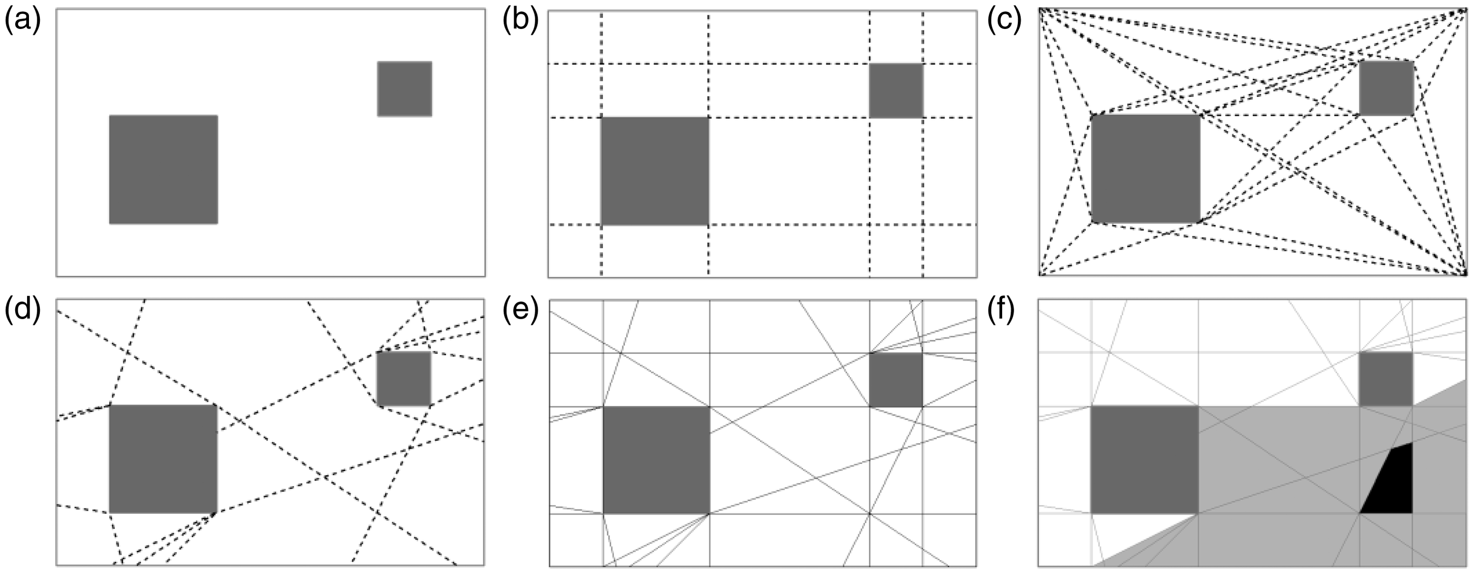
The visual relationship between e-spaces is conceptualised by determining the convex span of each e-space. The convex span of a specific e-space is the collection of e-spaces whereof each point in those e-spaces is fully visible from every point in that specific e-space (Peponis et al., 1997) (Figure 1(f)).
Endpoint partition graph
In this section, the implementation of the endpoint partition as wayfinding graph for landmark-based path-finding will be explained. The endpoint partition results in a collection of e-spaces for each room. Within a room, the e-spaces are connected through the collection of convex spans. However, within the context of landmark-based path-finding, these connections are only usable if they can be linked to a landmark. As mentioned earlier, landmarks can act as pointers or as beacons. In the first case, a navigator is able to use all possible connections in the convex span of an e-space in which a landmark is situated as the action can be linked associatively to that landmark. In the latter case, a navigator can be directed from an e-space towards another e-space wherein a landmark is situated if that e-space is part of the convex span of the first e-space. In other words, the landmark is visible. In addition, this beacon can be used to reach all other e-spaces that the line of sight between the current e-space and the beacon intersects. In this way, two nodes connected by an edge are mutually visible. In this way, these landmarks ensure the navigator that he or she is still on the correct route and allow error recovery (Michon and Denis, 2001). This is in line with Heiniz et al. (2012).
In addition, the size and shape of an e-space are taken into account because a person must be within one single e-space before the next wayfinding action begins. This means that e-spaces that are too small or are too narrow, so that a person does not fit into them, cannot be used to guide a person from A to B. We call these e-spaces ineligible. There are two reasons for this. First, if a person would be situated in more than one e-space, it is difficult to assess the visual relationship with other e-spaces as the convex span is defined for each e-space separately. Second, associative landmarks must be linked to a subarea (i.e. e-space) in which the object is visible from all possible locations within that subarea. To clearly link an action to a landmark associatively, the observer must be within the same subarea. In other words, only landmarks in eligible e-spaces can be used associatively because a person cannot be within an ineligible e-space due to its size and shape. Note that in this study the eligibility is based on the dimensions of a person, but other elements as wheelchair size can also be taken into account.
Following, the various rooms are linked through connectors (i.e. doors, elevators or staircases). These elements are not seen as spaces, but as edges connecting two eligible e-spaces closest to the connector, one in each room. In addition, these connectors are linked as a landmark to the e-spaces that spatially touch the polygons representing these features. This means that if the e-space, adjacent to the door, is not eligible, a door will be linked to two different e-spaces in a room: once as a landmark to the adjacent e-space, which is not eligible, and once as an edge to the closest eligible e-space. The use of doors, elevators and staircases as landmarks is motivated by the fact that they can easily function as reference points. The authors realise that as the number of doors in a room increases, it becomes more difficult to explicitly refer to a door as more similar objects are present. However, numerical chunking, which is a common principle when giving directions, can be used to specify a door (Klippel et al., 2003). Note that the various connections in the graph are considered equal in the assumption that a person can look around 360°. However, the connections originating from a specific e-space could be ordered based on direction (e.g. to avoid sharp turns or to take into account the field of vision) or saliency of the beacon(s) linked to the connections. Another possibility would be to take into account the distance between the observer and a landmark as landmarks at greater distances could be less distinctive or less usable as reference point.
Methods
In this method section, the landmark-based path-finding algorithm is explained. For the actualisation of the algorithm, the authors chose to implement the Python site-package ArcPy which enables the use of a broad range of geoprocessing tools of the ArcGIS environment developed by ESRI. The landmark-based path-finding algorithm consists of three steps (i.e. the endpoint partition, the construction of the e-graph and the generation of landmark-based paths) and builds upon three classes of geometric information provided by the user stored in a File Geodatabase. The workflow is visualised in Figure 2.
Workflow landmark-based path-finding algorithm.
The first two classes of geometric information are derived from an AutoCAD file that contains a detailed floor plan of the building. In addition, features like large pieces of furniture, cabinet work and sanitary fittings are also depicted on this floor plan. All elements that are part of the spatial structure of the building or may act as an obstacle are exported to a Shapefile. Next, this Shapefile is split and converted to two File Geodatabase Feature classes (i.e. ‘rooms and obstacles’ and ‘connectors’). Note that an obstacle is considered to be each spatial element that may obstruct the line of sight of a person in terms of visibility and/or movement (e.g. pillars). On the one hand, visibility has an impact on the construction of the e-spaces and their convex spans as this construction is based on the visual information provided by the surroundings. On the other hand, the algorithm calculates the visibility of a landmark based on the assumption that a navigator passes certain e-spaces along the line of sight (e.g. when walking towards a beacon). As such, objects that hinder movement must also be taken into account.
The first File Geodatabase Feature class represents the layout of the building. All rooms and obstacles within these rooms are represented through polygons. Based on the geometries of these polygons, the s-lines (see Algorithm 1) and d-lines (see Algorithm 2) are constructed for each room. The algorithms needed for the construction of these lines were written in Python based on the principles of the endpoint partition as proposed by Peponis et al. (1997). Next, these lines are transformed to e-spaces with the ArcPy function ‘Feature To Polygon (management)’. Following, the convex span statementis specified for each e-space. This is done by comparing each e-space to all other e-spaces in a room and verifying if all vertices of the first e-space are visible (i.e. the line of sight does not cross an obstacle) from all vertices of the second e-space. Creation of s-lines. Creation of d-lines.Algorithm 1
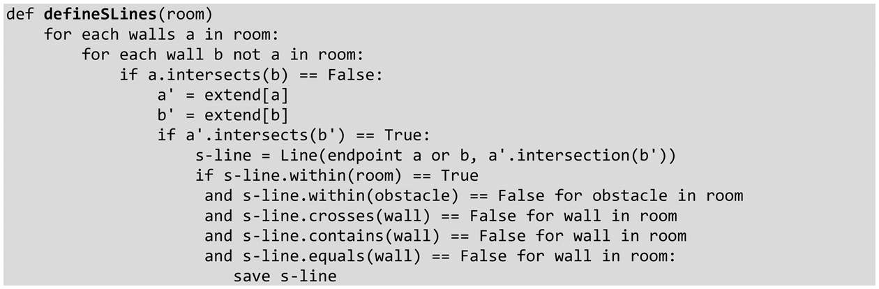
Algorithm 2
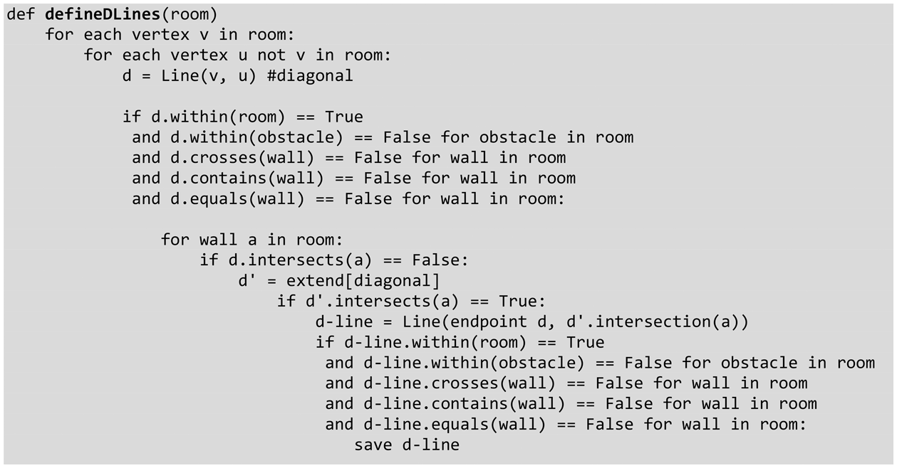
The second (File Geodatabase Feature) class contains polygons that represent the connections between the various rooms, namely doors, staircases and elevators. These connectors are used to link the collection of convex spans in each room to those in adjacent rooms. In this way, a graph is formed for the entire building. Note that the edges between the various rooms can be directed, while the graph edges formed by the convex spans are not as these are based on visibility.
The final class is a collection of landmarks. The concept of a landmark implies several cognitive aspects with respect to saliency and the mental map of the environment. Due to these aspects, landmark identification remains difficult. With respect to the proposed algorithm, however, a potential landmark must support the basic functionalities that are implemented in the algorithm. As such, each spatial object that can be used as an associative cue and/or as a beacon can be considered to be a landmark within the framework of this study. Based on this requirement, the connectors mentioned in the previous paragraph may also act as landmarks. However, as these connectors also act as edges that are part of the graph, they are grouped in a separate class and are indirectly integrated in the ‘landmark’ class (see Figure 2). In the File Geodatabase Feature class these landmarks are represented by points or polygons. The semantic attributes of each landmark are linked to the e-spaces in which they are situated. In addition, the landmark is represented by a point location (i.e. the point object itself or the centroid of the polygon) to determine the line of sight from one e-space, where an observer is standing, and the landmark. This line of sight is used to determine all e-spaces that are reachable when using the landmark as a beacon. Based on the e-graph, which connects the various e-spaces, the characteristics of the e-spaces (e.g. eligibility) and the used landmark set, the algorithm can calculate paths in line with the definition of landmark-based path-finding. This algorithm uses a breadth-first search to traverse a tree whereof the root is the wayfinders start location or node. The tree itself is constructed based on the guidelines mentioned in ‘Endpoint partition graph’ section (see Algorithm 3). The result of this breadth-first search is a tree in the form of a dictionary in which a parent is attributed to each e-space in the e-graph. By backtracking from the destination e-space up to the start e-space, the path that requires the least amount of steps (i.e. wayfinding actions linked to a landmark) between that destination and starting point can be determined. Application of breadth-first search (Skiena, 2012).Algorithm 3

Results: A case study
In this section, the results of a case study are presented to evaluate the usability of the proposed landmark-based path-finding algorithm. In this case study, characteristics of e-paths that are based on the e-graph will be compared with those of the corresponding shortest paths that are constructed using a geometric network model. These characteristics are (average) path length and path embedding. This network model represents a room by a single node. Linear elements (i.e. hallways) forming the network between rooms are represented by a sequence of nodes whereby each node provides a connection with the adjacent room near the natural access point of that room (e.g. door). This geometric model was used to calculate the shortest paths because an analogous comparison was made by Vanclooster et al. (2014). Here, the results of the least risk path algorithm were compared with those of the shortest path algorithm that was applied on Lee’s Geometric Network Model (Lee, 2004). In addition, the indoor test environment of this case study and the one used by Vanclooster et al. (2014) is the same, namely the Plateau-Rozier building in Ghent, Belgium. Various junctions in the building are characterised by a high level of connectivity. This emphasises the need for landmarks to unambiguously specify navigational instructions. In contrast, this study only focuses on the ground floor of the building for three reasons. First, the ground floor level is considered to be more complex. Second, it is more accessible for the general public compared to the other floor levels. Third, a large number of landmarks on the ground floor level are already identified (see Viaene et al., 2014). Note that it is possible to apply the proposed algorithm on multiple floor levels. In this case, the e-graph and related e-spaces must be calculated for each floor level separately. Next, these e-graphs can be linked to each other by the user with the help of a function that is part of the algorithm. This is done by specifying the e-spaces on the different floor levels that should be connected and by identifying the connector (e.g. elevator) connecting them. The landmark-based path-finding itself can then be applied on this combined e-graph of the building. As a final part of the case study, the impact of the landmark distribution across the building is examined by applying the algorithm with different sets of landmarks.
Comparing e-paths and shortest paths
For the Plateau-Rozier building, represented by 226 polygons (209 rooms or hallways and 17 obstacles within those rooms), the endpoint partition results in 230,141 edges and 9821 e-spaces with an average surface area of 0.81 m2 (standard deviation: 4.66 m2, minimum: 0.000003 m2, maximum: 130.23 m2). Based on the criterion that a person, represented by a circle of 0.5 m in diameter, must fit inside an e-space, 1295 e-spaces are eligible. In comparison, the geometric network model consists of 375 nodes and 884 edges. Following, a set of 109 landmarks is used (Figure 3), which is based on the analysis of concurrent thinking-aloud protocols generated by a group of navigators who traversed a route in the building twice (Viaene et al., 2014). These landmarks include amongst others large plants, display cabinets, art work, posters and vending machines. As mentioned earlier, doors, elevators and staircases are also used as reference points. In a next stage, all e-spaces are selected that are considered to be a potential starting point or endpoint for a navigator. For each room apart from hallways, the e-space that contains the node representing this room in the geometric network model is selected. This results in 191 locations that can function as start or endpoint of a path. Finally, landmark-based e-paths are calculated between all combinations of these locations. This results in 36,290 e-paths. Analogously, 36,290 shortest paths are calculated between those locations with a Floyd–Warshall algorithm. Note that the shortest path from A to B will be identical to the shortest path from B to A. As such, only 18,145 shortest paths are actually calculated. The e-paths, on the other hand, are not symmetrical as they depend on the visibility of landmarks, which is influenced by the travel direction.
Distribution of landmarks (normal landmark set).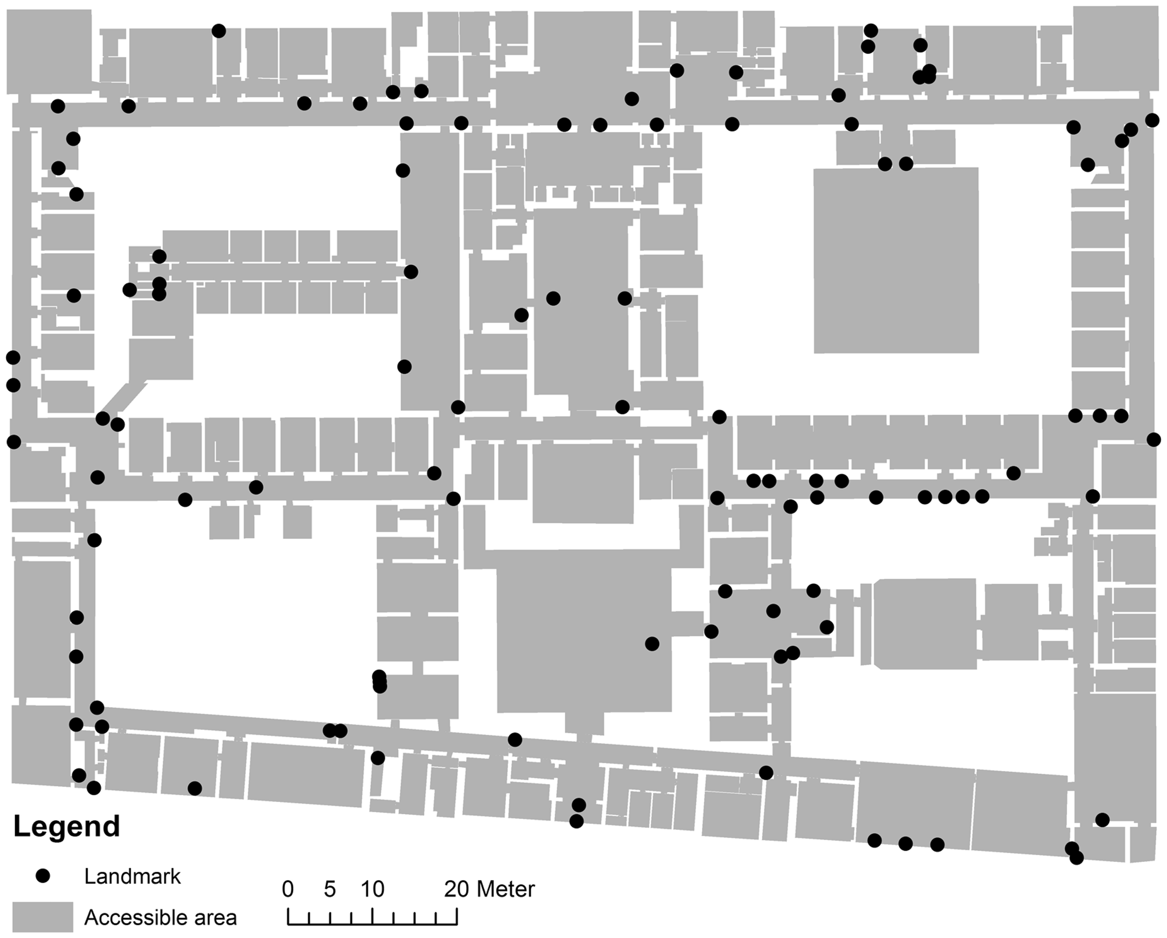
Disconnected locations
The proposed landmark-based path-finding algorithm is based on the principle that wayfinding actions must be linked to a landmark that can either be used associatively or as a beacon. An area with no or a very limited number of landmarks will be seen as a dead end by the algorithm. As such, the availability of landmarks may determine whether or not a destination can be reached. A destination that cannot be reached is called ‘disconnected’ as it will not be linked to the search tree on which the breadth-first search is applied. Applying the algorithm using the landmark collection shown in Figure 3 leads to the following results. In total, 1508 paths (4.16%) are not calculated because the start and end point could not be connected through landmark-based path instructions. Five endpoints (36, 199, 201, 245 and 251) are unreachable as they all account for 190 e-paths that are not calculated. Destinations 201, 245 and 251 are situated in ineligible e-spaces. As the algorithm will not direct a person into an ineligible e-space, these destinations are considered to be disconnected. However, the algorithm is able to direct a person to other (eligible) e-spaces in the rooms containing those destinations. Endpoints 36 and 199 are not reachable because of two reasons. First, the door is linked to two different e-spaces in the room: once as a landmark and once as an edge. Second, there are no other landmarks present in the room. For example, location 36 is situated in e-space 9647 (Figure 4). The door is linked as a landmark to the e-space adjacent to the door. As this e-space is not eligible, the door is linked as an edge to the eligible e-space closest to the polygon representing the door (i.e. e-space 7933). As such, a person can be guided to e-space 7933. However, as there are no other landmarks other than the door, which can only be used as a beacon and is not visible from 7933, a person cannot be guided to 9647.
Room with location 36.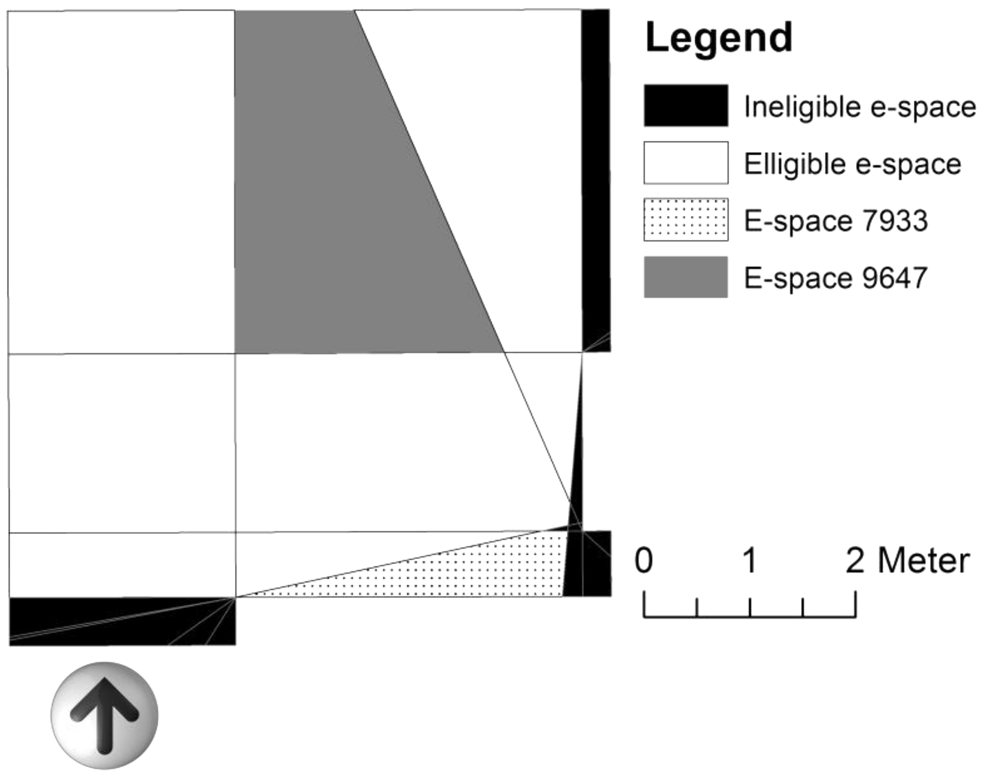
The remaining incalculable e-paths are linked to three specific locations functioning as start nodes, namely 36, 199 and 201. Again, these starting points are disconnected due to construction of the e-graph. For example, if a person is standing at location 36, which is situated in e-space 9647 (see Figure 4), he or she can be guided towards the door as the door functions as a beacon. However, the edge connecting the room to the hallway must be linked to the closest eligible e-space, namely e-space 7933. Additionally, the line of sight from the centre of e-space 9647 to the beacon (i.e. the door) does not intersect with e-space 7933. As a result, the person cannot be guided to the e-space that can be used to exit the room. This would only be possible if there are additional (visible) landmarks present in the room.
Path length
On the one hand, it is expected that an e-path will be longer compared to its corresponding shortest path. The algorithm will avoid low landmark density areas to generate paths that are easier to explain with the help of associative landmarks or beacons to adhere more to natural wayfinding behaviour. The average path length of the 34,782 calculated e-paths is 121.39 m with a minimum and maximum length of 1.14 and 308.12 m, respectively. The average path length of the corresponding shortest paths is 91.93 m (min. 1.15 m, max. 219.89 m). This means that a person going from A to B in this building following an e-path will walk a distance that is on average 32.04% longer than the shortest path leading from A to B. In total 27,626 e-paths were longer than their corresponding shortest path. Following, the minimum path lengths point out that an e-path can be shorter than its corresponding shortest path. As will be explained later, this is caused by the spatial models that were used to calculate these e-paths (i.e. e-spaces) and shortest paths (i.e. geometrical network model).
Table 1 shows that the path length increase can range over 100.00%. For example, the largest increase even amounts for 4506.98% as the e-path between destination 289 and 282 has a length of 238.84 m while the corresponding shortest path has a length of only 5.18 m (Figure 5). These locations are situated in an area that is characterised by a monotonous design and a lack of salient objects. Therefore, the landmark-based path-finding algorithm avoids this area. Moreover, the e-paths with the highest increase in path length all start or end in this area, which is situated between the main entrance hall (middle to of the map) and the central library. For example, the top 10 of e-paths with the highest length increase expressed in meters all start or end in this area. Additionally, the top five of e-paths with the highest length increase expressed in percentages start or end at destination 282. Another example is visualised in Figure 6. Here, the e-path deviates towards the centre of the building before entering the main entrance hall. In this way the low landmark density area following the entrance hall is avoided. In avoiding this area, a large detour is needed. The result is a path length of 228.18 m, while the shortest path found based on the geometric network model has a length of 62.80 m.
Path comparison between location 289 and 282 when applying a normal landmark set. Path comparison between location 30 and 285 when applying a normal landmark set. Path length difference of e-paths compared to corresponding shortest paths.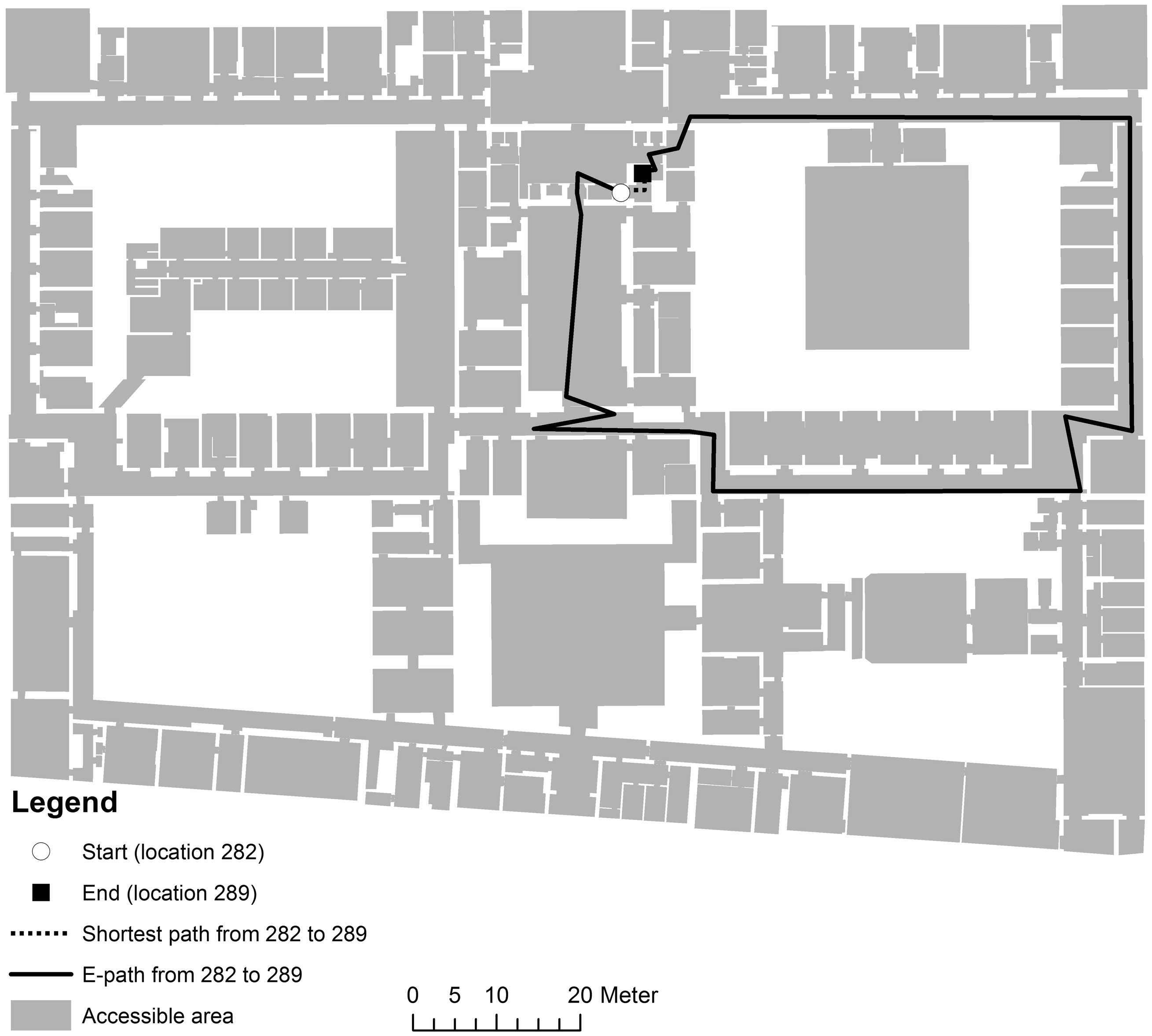

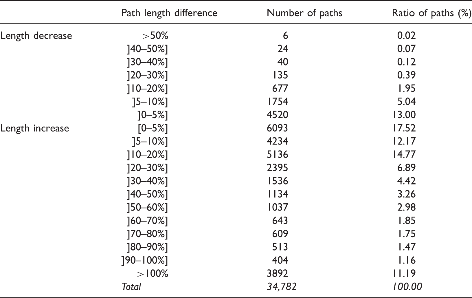
On the other hand, it can be expected that a proportion of e-paths will be shorter than their corresponding shortest routes due to the configuration of the network that is used to model the indoor environment. Depending on the spatial layout, the endpoint partition may decompose indoor spaces into smaller subspaces compared to the geometric network model. Providing that adequate landmarks are present, the endpoint partition allows cutting unnatural corners created by the geometric network model. As a result, an e-path may resemble the actual walking pattern of a navigator more closely. In this way, 7156 e-paths are shorter than their corresponding shortest path (see Table 1).
The impact of landmark distribution
The set of disconnected locations and the extreme path increase shown in Figures 5 and 6 demonstrate that the distribution of landmarks in the test environment has a serious impact on how the algorithm functions and the usability of the resulting e-paths. In this section, the use of two other landmark sets will be examined and compared with the landmark set that was used in the previous section (see Figure 3). First, the landmark-based path-finding algorithm will be applied using an empty landmark set. Only the available doors, elevators and staircases will function as reference points. It is expected that there will be a high number of disconnected locations in areas with few doors and that are characterised with short line of sights due to obstacles and hallway corners. In addition, the reduced availability of landmarks may lead to longer detours and an increased average e-path length. Second, the opposite situation, whereby a landmark is assumed to be situated in each e-space, will be examined. This is a fictional landmark set and is not based on real landmarks in the Plateau-Rozier building. This theoretical set is merely used to demonstrate the impact of the availability of landmarks on the proposed algorithm. In the case of this maximum landmark set, it is expected that the average e-path length will be similar to or even smaller than that of the calculated shortest paths as the e-paths can cut unnatural corners created by the geometric network model. In addition, there should be no disconnected location apart from 201, 245 and 251, which are situated in ineligible e-spaces.
When applying the algorithm with an empty landmark set in the Plateau-Rozier building, the calculated e-paths and corresponding shortest paths have an average path length of, respectively, 112.51 and 89.11 m. This average path increase of 26.25% is slightly lower than the increase of 32.04% that was present in the previous situation. This decrease in average path length increase is not in line with the assumption that a lack of landmarks would increase the average e-path length. In addition, fewer e-paths have a path length increase of 100.00% or more. An explanation can be found in the increase in disconnected locations. The results show that 18.67% of all possible e-paths (6776 routes) have a disconnected start point or endpoint. The same area as mentioned earlier is avoided again by the algorithm. Moreover, most paths starting or ending in this area could not be calculated. In other words, the paths that deviated the most from their corresponding shortest path in the previous section, whereby a normal landmark set was applied, are no longer included in the average e-path length. Following, all disconnected locations are situated in (a room adjacent to) an area where there are only a limited number of visible doors due to obstacles and bends in the corridor. Moreover, these doors can only function as beacons as they are linked to ineligible e-spaces.
After applying the landmark-based path-finding algorithm with a maximum landmark set, the results show that the number of disconnected locations is reduced. In this way, only 570 paths (1.57%) are not calculated due to locations 201, 245 and 251. The average path length of the 35,720 calculated e-paths is 103.94 m. That of the corresponding shortest paths is 91.98 m. Although, this increase of 12.99% is significantly lower than the increase observed in the previous situations, it is not in line with the assumption that, if enough landmarks are available, an e-path is shorter as the endpoint partition allows cutting unnatural corners created by the geometric network model. This increase, however, can be explained by the different aims of the algorithms that are used to generate the paths. While the Floyd–Warshall algorithm focuses on the edges of a network, as it is designed to reduce the total distance of a path, the breadth-first search focuses on the nodes of a network, as it minimises the number of steps or actions needed to reach a destination. As a result, areas that are characterised by a complex design with a lot of bends and obstacles will be avoided by the breadth-first search algorithm in favour of long straight hallways. While the shortest path may be shorter, it may take more instructions to explain. This is illustrated in Figure 7. Here, the shortest path traverses the centre of the building, which is composed of a large number of rooms. In contrast, the e-path takes a significant detour and follows the central hallway around the inner court. In total, the e-path is a sequence of 13 e-spaces connected by 12 path segments or instructions linked to a landmark. If an e-path would be constructed that respects the same sequence of rooms as the shortest path then 13 instructions would be needed, because the doors that need to be used are not mutually visible in two rooms and, therefore, additional information must be provided.
Path comparison between location 270 and 299 when applying a maximal landmark set.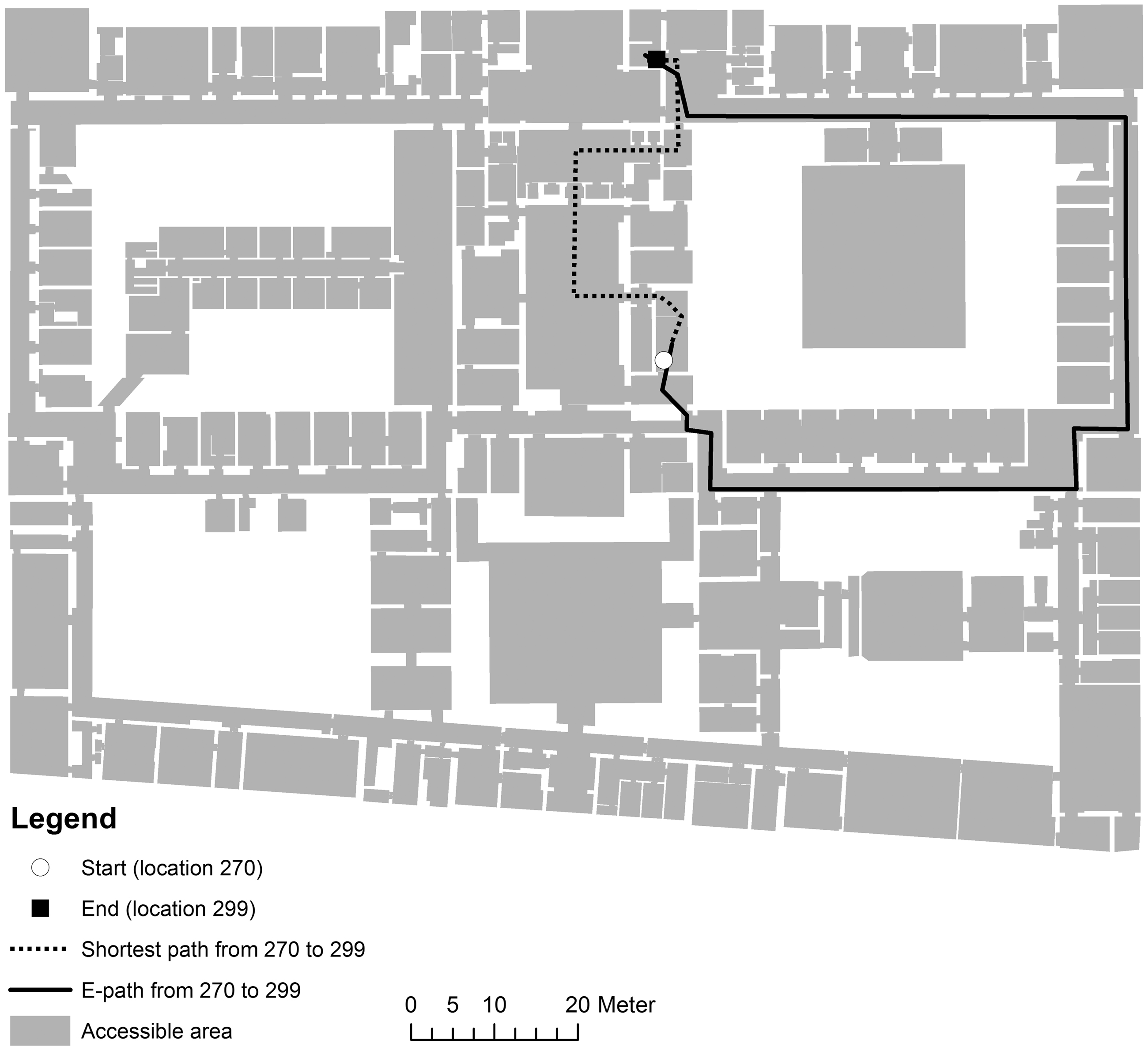
Discussion
In this section, the usability of the proposed landmark-based path-finding algorithm will be evaluated based on the results of the case study. We assume that the objective of the proposed algorithm is guaranteed, namely generating a path that can be explained by a minimum of actions linked to landmarks to reduce the cognitive load of the observed. In this way, the path-finding algorithms adheres to natural wayfinding behaviour and should result in paths that are easier to understand and follow, compared to the corresponding shortest path. However, these advantages must be weighed up against the disadvantages linked to the use of the endpoint partition graph as spatial model. These disadvantages include the high number of nodes generated by the endpoint partition, the inability to lead a person to a specific e-space (i.e. disconnected location) and the increased path length of the e-paths.
First, the endpoint partition resulted in 9821 e-spaces compared to the 375 nodes needed to model the indoor environment with the geometric network model. This more detailed subspacing can be used to guide a person to specific regions within a room and around obstacles. However, a large proportion of these e-spaces were ineligible. As such, a person could not be guided to these e-spaces. This limited the ability to guide a person to specific areas in a room, even if there were enough landmarks present to guide a person to that area. Moreover, this high amount of ineligible e-spaces was still part of the path-generating process, as they may have contained landmarks that could function as beacons. The complexity of the breadth-first search algorithm can be expressed as O(|V| + |E|) with V being the number of vertices and E the number of edges. As a result, a higher number of vertices and edges (i.e. e-spaces and their connections) increases complexity and the time needed to calculate a path. For these reasons, more research should be conducted to find ways to deal with these ineligible e-spaces. For example, small e-spaces could be combined on a higher hierarchical level so that they can be used for guidance, while the e-spaces on a lower level can still be used to handle the spatial information that can be observed when a transition occurs from one e-space to another.
Second, the results show that when no landmarks were available apart from reference points as doors, elevators and staircases, 18.67% of the possible e-paths cannot be calculated. The implementation of the algorithm with a maximal landmark set showed that 1.57% is due to the fact that the path led to an ineligible e-space and could not be attributed to a lack of landmarks. In a normal situation with a set of previously identified landmarks, 4.16% of all possible paths were not calculated, which is not negligible. However, these disconnected locations could easily be ‘connected’. On the one hand, these disconnected locations were due to the fact that they were located in ineligible e-spaces (i.e. locations 201, 245 and 251). However, one could assume that a person is not interested in reaching a specific area that is smaller than a circle of 0.5 m, but in reaching the room in which that e-space is located or the area around that specific e-space. For locations 245 and 251, the algorithm was able to guide a person to the e-spaces adjacent to the e-spaces containing these locations. On the other hand, the cause of these disconnected locations was the way the e-graph is constructed, namely the fact that a door can be linked to two different e-spaces, once as a landmark and once as an edge. This was the case for locations 36, 199 and 201. In all of these cases, this can be resolved by an additional beacon in the e-space to which the door is linked as an edge or an associative landmark that is visible from that e-space and from the e-space in which the person is standing. As these e-paths were linked to only three disconnected locations, it is attainable to resolve this issue by creating three additional reference points.
A third disadvantage is the increased path length. A fifth (20.41%) of all e-paths were more than 50.00% longer than their corresponding shortest path and 11.19% were over 100.00% longer than the corresponding shortest paths. In ideal circumstances with a plenitude of visible landmarks, the average path increase was reduced to 12.99% and 91.87% of the e-paths were less than 50.00% longer or even shorter than the corresponding shortest path. This is comparable to an outdoor study of Duckham and Kulik (2003) in which ‘simplest’ paths had an average length increase of 16% and more than 90% of simplest paths were less than 50% longer than the corresponding shortest paths. Duckham and Kulik (2003) found this acceptable as the ‘simplest’ path adheres more to natural wayfinding behaviour because the related route instructions are easier to comprehend. In addition, these path instructions do not rely on metric information. The same can be said for the e-paths presented in this paper. Another principle of the proposed landmark-based path-finding algorithm is the minimisation of the number of instructions (linked to landmarks) needed to guide a person. Reducing the instruction length is also an important feature of the simplest instruction algorithm proposed by Richter and Duckham (2008) in an outdoor environment. They found that a simplest instruction path was on average 13% longer compared to the shortest path. This was found acceptable in light of the reduced complexity of the route instructions. Furthermore, only 6.7% of the simplest instruction paths were more than 25% longer than the shortest path and 75.9% were less than 15% longer than the shortest path. With respect to the maximal landmark set, 19.02% of all e-paths were more than 25.00% longer and 70.20% were shorter or less than 15.00% longer than the shortest path. Although, the e-paths showed an increased number of routes that were significantly longer, especially with a normal landmark set, these ratios are similar. Finally, in the previously mentioned study of Vanclooster et al. (2014), which took place in the same indoor environment as this study, 98% of the least risk paths had a deviation with a smaller path length increase than 25% of the corresponding shortest path. In this study, this can be said for 80.98% of all e-paths when using a maximal landmark set and 68.97% using a normal landmark set. On average the least risk paths only had a path length increase of 4% compared to the shortest paths, which is significantly lower than the length increase found in this study. In general, we conclude that the path length increase is comparable to other richer cognitive algorithms. However, one must note that a lack of landmarks can have a serious impact on the maximal path length increase. As such, the landmark-based path-finding algorithm is less stable and more dependent on environmental features than the simplest path, simplest instruction and least risk path algorithm.
Conclusion
In this paper, a landmark-based path-finding approach was proposed to reduce indoor path complexity. As part of this approach, this paper elaborated on the endpoint partition, which was implemented as spatial model. This partition was developed by Peponis et al. (1997) to describe the spatial configuration of an indoor environment in a mathematically defined way in relation to the visibility of features that characterise the spatial layout of a building. Following, it was examined whether the combination of this landmark-based approach and this spatial model was able to generate reasonable paths to lead a person from an origin to a destination in terms of path length. The results show that the landmark-based path-finding algorithm is able to define a path, based on a minimal amount of actions linked to landmarks, while the path length increase compared to the shortest path is similar to the length increase observed when applying the simplest path, simplest instruction or least risk path algorithm. Therefore, the proposed algorithm may function as a valuable alternative for Dijkstra’s shortest path algorithm in order to resolve indoor wayfinding problems by providing paths that adhere more to natural wayfinding behaviour. In contrast to these other cognitive algorithms, however, the landmark-based path-finding algorithm is highly dependent on the availability of visible landmarks to limit the maximal path length increase and on the spatial configuration of the building to minimise the amount of ineligible e-spaces. These two elements may result in the impracticability of the proposed algorithm. Future research will focus on handling these ineligible e-spaces to increase the employability of the endpoint partition. In addition, cognitive studies with human subjects will be conducted to confirm the assumption that the calculated e-paths are more in line with natural wayfinding behaviour compared to their corresponding shortest paths. Furthermore, these e-paths will be compared with paths generated by existing algorithms that support natural wayfinding (e.g. simplest paths) in order to assess the value of the proposed landmark-based path-finding algorithm with respect to these approaches. Finally, as landmarks can be identified indoors and outdoors, future research will implement the presented landmark-based path-finding algorithm to offer seamless wayfinding services between indoor and outdoor space.
Footnotes
Declaration of conflicting interests
The author(s) declared no potential conflicts of interest with respect to the research, authorship, and/or publication of this article.
Funding
The author(s) disclosed receipt of the following financial support for the research, authorship, and/or publication of this article: This work was supported by the Flanders Research Foundation (FWO-Vlaanderen) (FWO14/ASP/293).