
Abstract
The FLORIS (FLOw Redirection and Induction in Steady-state) model, a parametric wind turbine wake model that predicts steady-state wake characteristics based on wind turbine position and yaw angle, was developed for optimization of control settings and turbine locations. This article provides details on changes made to the FLORIS model to make the model more suitable for gradient-based optimization. Changes to the FLORIS model were made to remove discontinuities and add curvature to regions of non-physical zero gradient. Exact gradients for the FLORIS model were obtained using algorithmic differentiation. A set of three case studies demonstrate that using exact gradients with gradient-based optimization reduces the number of function calls by several orders of magnitude. The case studies also show that adding curvature improves convergence behavior, allowing gradient-based optimization algorithms used with the FLORIS model to more reliably find better solutions to wind farm optimization problems.
Introduction
Optimizing wind farm layout is a major topic of investigation and has proceeded along two main fronts: wake model development and optimization algorithm development. This work connects these areas of study by focusing on taking an existing wake model and adjusting it to work more effectively with gradient-based optimization algorithms with the intent of reducing the computational cost of wind farm optimization and more reliably producing good solutions to wind farm optimization problems.
Grouping wind turbines in wind farms reduces the cost of infrastructure, but has the negative result of reducing the overall efficiency of a wind farm due to wake effects (Herbert-Acero et al., 2014). Wind turbines convert the kinetic energy from the wind into electrical energy and obstruct the air flow, causing the wind to slow down and become more turbulent. The region of slower, more turbulent air downstream of a wind turbine is called the wake. The wake of a wind turbine has been measured to persist as far as 30 times the turbine’s rotor diameter downwind, though by 10 rotor diameters downwind the wind velocity in the wake is similar in magnitude to the natural variations in the wind stream (Hirth et al., 2012). If a turbine is in the wake region of another turbine, the turbine in the wake region will have a much lower electrical energy output than it would were it fully in the freestream flow. The wake effects are compounded for large wind farms, resulting in a significant decrease in wind farm efficiency and an increase in the cost of energy.
Because the amount of energy converted from the wind into electrical energy by a wind farm is primarily dependent on the wind speed, and the wind speed is greatly reduced in wake regions, designing a wind farm’s layout and control method to minimize wake effects is crucial. One way to improve wind farm efficiency is through cooperative control using either blade pitch or yaw. Both of these cooperative control methods reduce the efficiency of the front turbine(s) in order to increase the efficiency of the downstream turbine(s). Cooperative control has been shown to have significant benefits for certain combinations of turbine spacing and wind speed (Abdulrahman and Wood, 2015), and the potential of cooperative yaw control has been shown in simulations to have a greater impact than cooperative control based on axial induction (Gebraad et al., 2015). The theory behind yaw control was presented by Jiménez et al. (2010), who also presented large eddy simulations (LES) demonstrating the effects of yaw on wake deflection. Recent field measurements do indicate that wake deflection may be more sensitive to small wind direction changes than was indicated in the LES (Fleming et al., 2017; Marathe et al., 2016), but cooperative control with turbine yaw still seems to have significant potential. It may be possible to improve the energy production of an existing wind farm using cooperative control through either blade pitch or yaw. However, including the effects of cooperative control in the initial design may further improve wind farm efficiency (Gebraad et al., 2017).
Wake effects are predicted using wind turbine wake models that approximate the fluid state downwind of a wind turbine or multiple wind turbines. Many different models of varying accuracy, capability, and fidelity are available in the literature (Bastankhah and Porté-Agel, 2016; Crespo et al., 1999; Gebraad et al., 2014; Göçmen et al., 2016; Herbert-Acero et al., 2014; Larsen, 2009). Wake models are used in various aspects of the design and analysis of wind farms, especially in the layout design (Crespo et al., 1999). Deflection due to wind turbine yaw is typically neglected in engineering wake models, though some models including the effects of turbine yaw have been proposed (Bastankhah and Porté-Agel, 2016; Gebraad et al., 2014; Herbert-Acero et al., 2014). The FLORIS (FLOw Redirection and Induction in Steady-state) model, a parametric wind turbine wake model that predicts steady-state wake characteristics based on wind turbine position and yaw angle (presented by Gebraad et al., 2014), incorporates the theory presented by Jiménez et al. (2010) to include wake deflection due to yaw. Because the FLORIS model includes yaw, it is a candidate for use in a wide variety of wind farm optimization problems.
Most wind farm optimization problems are solved using genetic algorithms or other gradient-free optimization methods (Herbert-Acero et al., 2014; Moorthy et al., 2014). Gradient-free methods are good at handling cases with multiple local minima, as is the case for wind farm optimization. However, gradient-free methods are not as effective when dealing with the hundreds to thousands of design variables in a typical wind farm optimization problem. Because of this weakness in gradient-free optimization methods, wind farm layout optimization has been limited to relatively small numbers of wind turbines and few wind directions.
In contrast to gradient-free methods, gradient-based optimization algorithms (optimization algorithms that make use of a knowledge of the partial derivatives of the design space) are not well suited to problems with many local minima, but are well suited to problems of high dimensionality. In other words, gradient-based methods may not find the global optimum (though global optimality is not guarenteed using gradient-free methods either), but they can work well with the number of design variables present in the problems associated with wind farm design. Gradient-based methods are also able to converge to within a tighter tolerance of a given optimum than most gradient-free methods. A combined approach, beginning with a gradient-free optimization to avoid local minima and transitioning to a gradient-based method for refinement, has been successfully demonstrated using TOPFARM (Réthoré et al., 2014), a wind farm optimization tool under development by DTU Wind Energy (Larsen et al., 2011). This approach has the advantage of likely avoiding local minima (using the gradient-free method) and, afterwards, converging accurately and relatively quickly to a refined final solution (with the gradient-free method). One important drawback of this approach is the excessive computational cost for the gradient-free methods when there are many design variables (Réthoré et al., 2014).
Gradient-based optimization methods require the objective function to be differentiable and Lipschitz continuous (Herbert-Acero et al., 2014). Most engineering wake models do not meet these criteria, and even the wake models that do meet these requirements do not provide exact gradients. Gradients can be approximated with numerical methods, such as finite difference, but if a wake model is not smooth, then numerical methods may not be effective. Because the gradients are not supplied by the existing models, numerical approximation methods must be used if a gradient-based optimization approach is desired. Numerically approximating the gradients significantly increases the required number of function calls to converge an optimization problem and can decrease the accuracy of the final solution.
Some wake models also have regions of non-physical zero gradient (flat areas) that can cause premature convergence. To take full advantage of gradient-based methods, we need a simple engineering wake model with exact gradients and no flat regions in the wake.
The FLORIS model is a computationally efficient wake model and has been used in wind turbine yaw control research (Fleming et al., 2017; Gebraad et al., 2014; Gebraad and Van Wingerden, 2014), as well as in wind farm optimization (Fleming et al., 2015b; Gebraad et al., 2017; Thomas et al., 2015; Tingey et al., 2015). The FLORIS model is simple enough that obtaining exact gradients is a reasonable proposition, and while the FLORIS model does have flat regions, this article shows that the flat regions can be adjusted to give appropriate curvature. Having a version of the FLORIS model with appropriate curvature and exact gradients will enhance optimization studies performed with the model by allowing the use of exact gradients with optimization algorithms, reducing the number of function calls, potentially reducing the time required to converge, and improving solution accuracy for large wind farm optimization problems.
This article presents (1) a brief explanation of the original FLORIS model, (2) changes made to the FLORIS model to improve compatibility with gradient-based optimization methods, and (3) a series of case studies comparing the performance of gradient-based wind farm optimization with each change to the FLORIS model.
The FLORIS wake model
A brief explanation of the FLORIS model
The FLORIS model is a derivative of the Jensen (or Park) wake model (Jensen, 1983) and the wake deflection model presented by Jiménez et al. (2010). The FLORIS model defines three zones within the turbine wake as shown in Figure 1. The overlap area of each zone with a downstream turbine’s rotor-swept area is used to estimate the effective wind speed of downstream turbines. Each of the wake zones has a uniform crosswind velocity profile and a unique velocity deficit decay rate. The offset and velocity deficit of the wake are determined by the yaw and relative position of the turbine. The FLORIS model parameters are tuned using data from high-fidelity, LES-based computational fluid dynamic simulations performed with the Simulator for Onshore/Offshore Wind Farm Applications (SOWFA) (Fleming et al., 2015a). While details of the parts of the original FLORIS model that have been altered in this work are provided in the following section, a full explanation of the original FLORIS model can be found in the work of Gebraad et al. (2014).
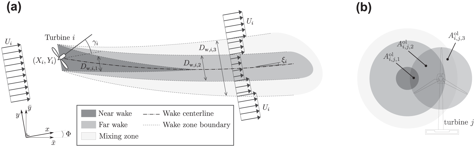
The FLORIS wake model uses three wake zones and predicts their expansion (resulting in predicted wake zone diameters,
Equations affected by the changes to the FLORIS model
Wake center
The original FLORIS model defines the wake center as

where the three terms represent the crosswind location of the turbine (

where

where

Wake diameter
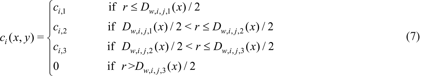
The diameter of each zone

where
Velocity deficit
The velocity in the wake is defined as

for
where

where
Changes to the FLORIS wake model
Several changes to the FLORIS model are presented here that provide the characteristics important for gradient-based optimization. The changes include removing a discontinuity, adding curvature to areas of non-physical zero gradient, obtaining exact gradients, and re-tuning the FLORIS model parameters to account for the other changes. However, two changes were made to the wake center definition of the FLORIS model prior to this work. All other changes presented are in addition to the following changes in the wake center definition.
Prior changes to the wake center definition
The redefinition of the wake center changed the second and third terms of equation (1). In the original model, the wake center offset due to rotor rotation increased linearly with downstream distance. In the current FLORIS model, the linearly increasing offset has been removed from equation (2) as follows

The current FLORIS model also redefines the initial wake angle (

These changes to the wake center definition make the FLORIS model more realistic by allowing all deflection effects induced by the rotor to decay as the wake moves downstream, as shown in Figure 2.

(a) Position of the wake center (yw) of turbine A in the crosswind direction at the downstream location of turbine B. The turbine causing the wake is located at (0,0). Changes made to the wake center definition of the FLORIS model allow the wake center line to become parallel to the freestream. The linear increase in wake center offset has been removed and a constant value has been added to the initial wake angle. (b) Plotting context for (a) and some following figures. Turbine A is located at (0,0). Turbine B starts at (0,0) and moves along the x-axis.
Discontinuities
To determine what changes should be made to the FLORIS model for improved compatibility with gradient-based optimization, the design space of the FLORIS model was investigated by checking each of its equations analytically and by plotting slices of the design space. Two regions with discontinuities were identified.
Discontinuity across the rotor region
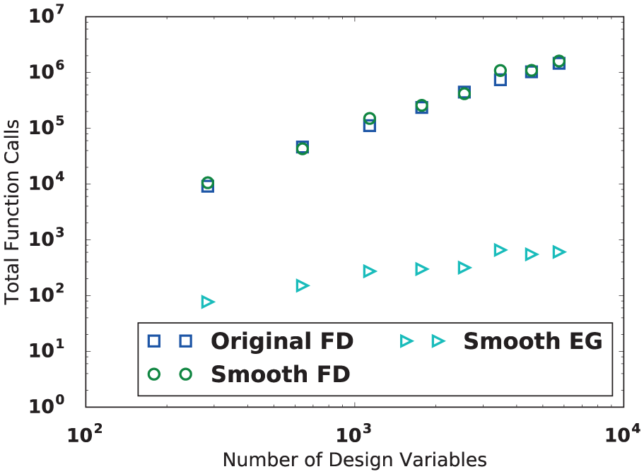
The FLORIS model, like most engineering wake models, does not define a transition from the freestream velocity to the lowest wake velocity, immediately behind the rotor. Because of this, there is a discontinuity across the rotor location in the freestream direction as shown in Figure 3.
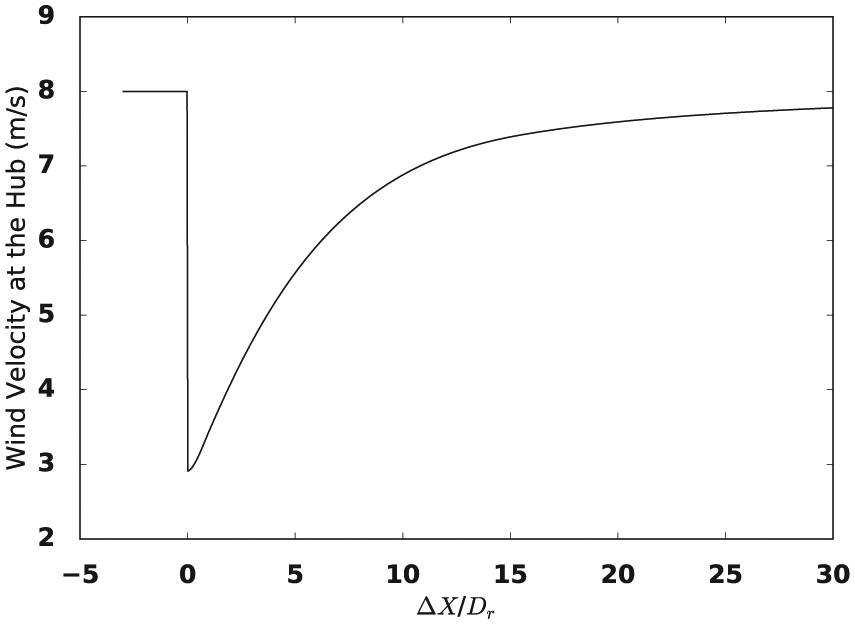
Discontinuity present in the wake velocity definition across the rotor in the downstream direction as seen by a second turbine. Plotted according to Figure 2(b).
While wind turbines are never placed closer than about two diameters in final designs, infeasible designs may be tried by the optimization algorithm (Belegundu and Chandrupatla, 2011; Gill et al., 2005). This means that even if a constraint is placed on the turbine proximity, the optimization algorithm may try to place turbines closer than is allowed in the final design while it searches for the optimal solution.
The case where turbines are closer than allowed in the final design was tested for convergence problems within an optimization context by placing four turbines incrementally closer and running a layout optimization. As long as no turbines were placed closer than
Discontinuity in the first derivative of the inner wake zone
Because the inner wake zone contracts linearly with downstream distance, the max function in equation (5) causes a sharp change in the first derivative of the inner wake zone as the zone’s diameter becomes zero. To facilitate effective use of exact gradients, the max function was replaced with a Hermite cubic spline that smoothly transitions the inner wake diameter to zero. The spline extends two rotor diameters parallel to the wind direction and is centered at the location where the inner wake diameter originally became zero. The equation for the center of the spline is

where
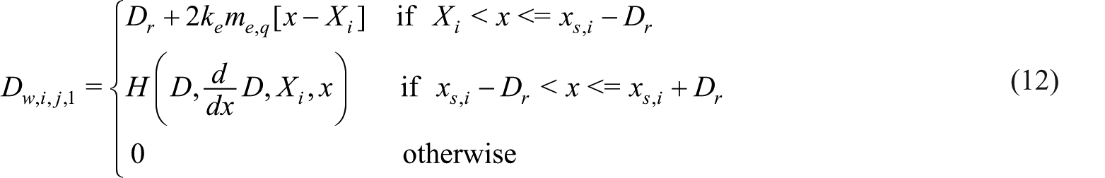
where
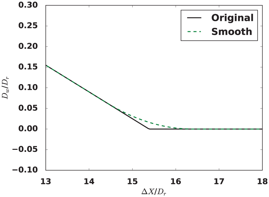
Changes made to remove the discontinuity in the first derivative of the inner wake diameter. Plotted according to Figure 2(b).
Non-physical regions of zero gradient
The three zones used to define the wake in the FLORIS model have the side-effect of creating regions within the wake with no change in effective hub velocity of a shadowed turbine for small changes in the turbines’ crosswind positions, as shown in Figure 5(a)-inset. While such a formulation does not present serious problems for analysis, it can cause premature convergence during gradient-based optimization (demonstrated in case study 2: linear wind farm).
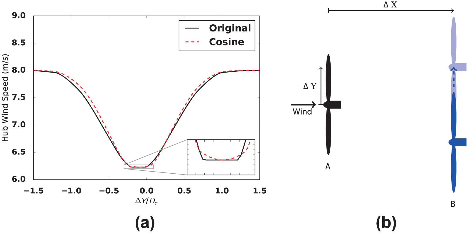
(a) Crosswind velocity profiles of the wake of turbine A as seen by turbine B at X = 7Dr comparing the FLORIS model with and without the cosine term. Freestream wind velocity is 8 m/s. (b) Plotting context for (a). Turbine A is located at (0,0). Turbine B moves crosswind from (∆X, –1.5Dr) to (∆X, 1.5Dr).
To add curvature to the flat regions, a cosine factor, similar to the one proposed by Jensen (1983), was added to the wake coefficient formulation of the FLORIS model. The cosine factor is defined as

where

where

The crosswind velocity profile as seen by a downwind turbine using the FLORIS model with and without the cosine factor is shown in Figure 5(a).
The cosine factor slightly reduces the wake deficit, with greater reductions at greater radial distances from the wake center such that all wake regions exhibit a slope away from the wake center. The cosine factor does not alter the wind velocity in the center of the wake. The cosine factor removes the non-physical regions of zero gradient while maintaining a good fit with the data used for tuning. Setting
Exact gradients
Exact gradients of the altered FLORIS model were obtained using algorithmic differentiation. The FLORIS model was re-written in Fortran 90 and algorithmic differentiation was performed using the Tapenade automatic differentiation tool (Hascoët and Pascual, 2013). The gradients of peripheral elements of the optimization problems under investigation were derived analytically. The gradients were combined using OpenMDAO, a Multidisciplinary Design Analysis and Optimization platform (Gray et al., 2010).
Re-tuning the FLORIS model
The altered FLORIS model was re-tuned by hand to the SOWFA data used to tune the original FLORIS model. One parameter was changed, and two were added. The parameter change was needed in order to counteract the reduction in the velocity deficit caused by the cosine term, it simply increases the diameter of the far wake zone (zone 2). The parameter adjustments are presented in Table 1. The resulting fit compared to the SOWFA data and to the original model is shown in Figure 6.
Changes to the FLORIS model parameters.

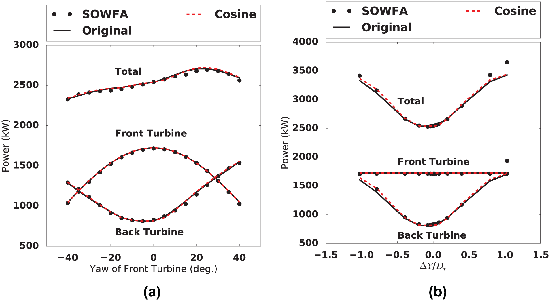
Comparison of the FLORIS model to SOWFA data for two wind turbines spaced at 7Dr in the downwind direction. (a) Comparison to SOWFA data for sweeping the yaw of the upstream turbine. (b) Comparison to SOWFA data for sweeping the crosswind location of the upstream turbine.
Coupling FLORIS with a rotor model
Another addition has recently been made to the FLORIS model to improve the accuracy of the annual energy production (AEP) calculations with the FLORIS model (Gebraad et al., 2017). The original model is accurate only when the turbines are operating in the Region 2 control operating point with fixed blade pitch angle and tip-speed ratio (Gebraad et al., 2017). The addition consists of coupling the FLORIS model with a rotor model that includes the turbine control policy based on blade pitch and rotor speed. The rotor model relies on pre-computed data calculated using the WISDEM CCBlade Blade Element Momentum (BEM) code (Ning, 2013, 2014). Using the pre-calculated data from CCBlade, the FLORIS model can correctly account for the full range of wind speeds. Because the rotor model requires the effective velocity at the turbine hub as an input, an iterative method is used to solve for the final hub velocities. The iterative solve and the inclusion of the control policy result in a more accurate inflow velocity for waked turbines.
While the added rotor model improves the FLORIS model, comparisons to it are not included in this study. As compared to the other model changes, this is a much more significant change to the physics, making the optimal numerical values less directly comparable. Because the purpose of this study is not to quantify the accuracy of the physics, but rather to understand the impact of the model formulation on efficient optimization, the rotor model was omitted in the following case studies. All case studies were run with the rotor model variant as a check, but results were similar to the cosine variant and did not yield additional insights. Its omission is for clarity in presenting results and not because it is any less effective for optimization. It remains the most accurate and recommended model for analysis and optimization use, and has been used in a related large-scale optimization study (Gebraad et al., 2017).
Case studies
We performed three case studies to compare the abilities of the original FLORIS model and the FLORIS model with the changes presented above. The optimizations in each case study were performed using SNOPT (Sparse Nonlinear OPTimizer), a gradient-based optimization algorithm that uses a sequential quadratic programming approach that is well suited to non-linear problems with high dimensionality (Gill et al., 2005).
The wind rose used in case studies 1 and 3 is based on measurements from the NoordZeeWind meteorological mast (Brand et al., 2012) from 1 July 2005 to 30 June 2006. The measurements were binned into 72 directions and the average wind speed for each direction bin was calculated. The probability wind rose is shown in Figure 7(a) and the directionally averaged wind speeds are shown in Figure 7(b). Three wind directions in this data set have a negligible probability and/or average wind speed—these three directions were not included in the calculations. AEP was calculated based on the power production for each wind direction weighted by the probability of the corresponding wind direction times the number of hours in a year using the average wind speed for each of the 69 included direction bins.
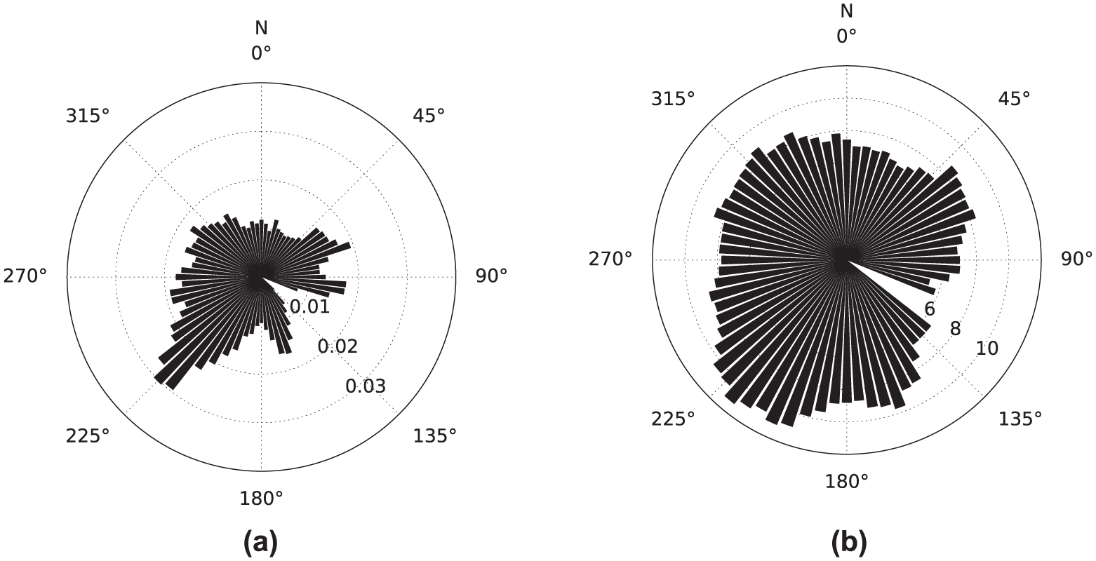
Wind data for case studies 1 and 3. These data are from the NoordZeeWind meteorological mast (Brand et al., 2012). (a) Directional probability. (b) Directionally averaged wind speed (m/s).
Five variants of the FLORIS model, representing steps in the changes to the FLORIS model presented above, were investigated in the case studies. In the variant names, EG stands for exact gradients and FD stands for finite difference. “Smooth” denotes the FLORIS model including the spline discussed in the section Discontinuity in the First Derivative of the Inner Wake Zone. “Cosine” refers to the FLORIS model including both the spline and the cosine term discussed in sections Discontinuity in the First Derivative of the Inner Wake Zone and Non-Physical Regions of Zero Gradient, respectively. All the model variants investigated, except the original model, include the wake center changes discussed in the section Prior Changes to the Wake Center Definition. The variants of the FLORIS model included in the case studies are outlined in Table 2.
FLORIS model variants used in the case studies.

Case study 1: scaling
Methods
This case study tests three variants of the FLORIS model (Original FD, Smooth FD, and Smooth EG) by optimizing a wind farm based on a simple
The objective function was formulated as
where
When yaw and position for each wind direction and turbine are used simultaneously, the numbers of design variables and constraints increase rapidly with more turbines. The coupled approach was used to demonstrate the ability of the gradient-based optimization to handle a large number of design variables with fewer function calls when using exact gradients. The numbers of turbines, design variables, and constraints for each run are shown in Table 3.
Dimensions of the cases used in Case study 1: scaling.

Each optimization was run until the first-order optimality (the norm of the Lagrangian) was within
Results and discussion
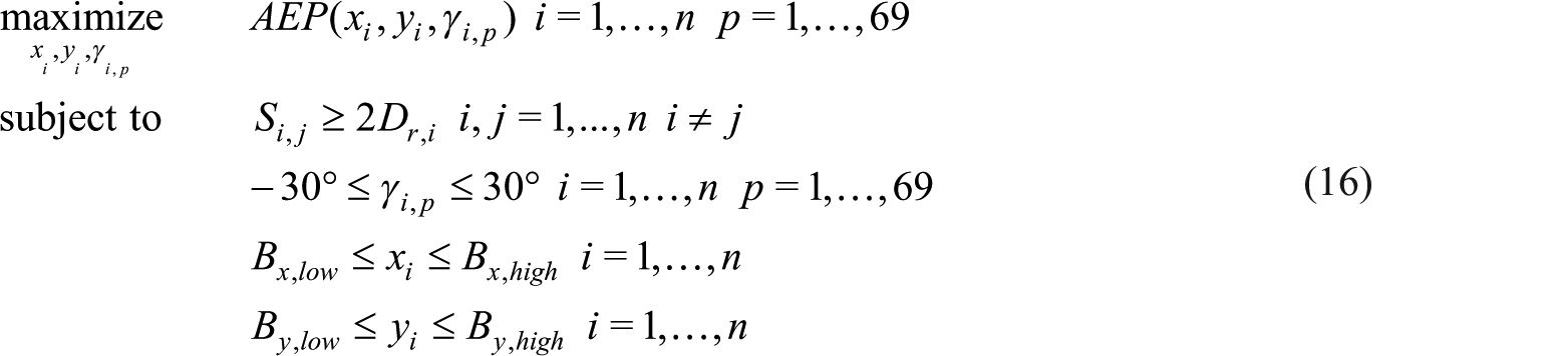
Only small changes in the turbine positions were seen in the optimization results, while significant changes were made in the yaw. The relatively small movement in positions is likely due to the starting positions, which fall within the optimal range suggested by Patel (2006) (though other arrangements, such as staggered rows, have been shown to be relatively optimal (Ammara et al., 2002; Fleming et al., 2015b; Moorthy et al., 2014)). Despite starting near a solution known to be reasonably optimal, the optimization algorithm was able to achieve significant improvements in AEP, between 1% and 7%, with greater AEP improvements for larger wind farms. The final percent AEP improvement was similar for each variant.
The number of function calls was recorded for both the objective function and the gradient function, if applicable. In Figure 8, it can be seen that the smoothing changes, while important for obtaining exact gradients for use with SNOPT (Gill et al., 2005), made little difference in the required number of function calls when used with finite-difference gradients. However, Figure 8 also shows that using exact gradients drastically reduced the number of function calls required to converge, with greater reductions for larger numbers of design variables.
Function calls required to converge with increasing number of turbines for the original, smooth with finite-difference gradients, and smooth with exact gradients versions of the FLORIS model.
The time required to converge does not necessarily scale by the same ratio as the number of function calls. In this case, where there are more design variables than constraints, we use an adjoint method to compute the total system derivatives (Martins and Hwang, 2013). The adjoint method requires solving a linear system for each constraint, and with many design variables (large linear system) and many constraints (many repetitions), this can become a significant cost if not managed carefully. By exploiting sparsity in the constraints, and skipping unnecessary gradient computations of highly inactive constraints, using exact gradients should be significantly faster than using finite differences for all of these analyses. We report function calls rather than time in this study because time is dependent on too many things that are not easily generalized (e.g. hardware, number of processors, the implementation of the gradient computation, and the optimization method).
Case study 2: linear wind farm
Methods
As noted in the section Non-Physical Regions of Zero Gradient, the regions of zero gradient in the FLORIS model can cause premature convergence during optimization. One simple case where this is readily apparent is during unidirectional, position-only optimization when the turbines begin in the center of other turbines’ wakes as shown in Figure 9. The FLORIS model uses an overlap ratio of the rotor area to the area of each wake zone to calculate the wake deficit. However, as can be seen in Figure 9(b), there are regions where the overlap ratio is constant for small movements of the rotor position. These regions are what cause the gradient of the velocity in the crosswind direction to go to zero as shown in Figure 5. When the partial derivative of the objective function in a given direction is zero, a gradient-based optimization algorithm will not move in that direction. For the case of interest, this means that the waked turbines will not be moved out of the wake(s). The curvature added through the cosine term provides the necessary information for a gradient-based optimization algorithm to move turbines out of other turbines’ wakes. The three turbines in this case study are spaced seven rotor diameters downstream of each other and offset from the first turbine in the crosswind direction so they are each in the center of the preceding turbine’s wake (a crosswind offset of −0.095Dr and −0.19Dr for the second and third turbines, respectively) as shown in Figure 9(a). The Smooth FD and Smooth EG FLORIS model variants were excluded from this case study for simplicity since they exhibited the same behavior as the original model.
Starting layout and wake cross section for case study 2: linear wind farm. Wind is from the left at 8 m/s. (a) and (b) share the color bar and legend. (a) Starting layout for the in-line optimization study. Turbines are separated by 7Dr in the downstream direction and centered in the next turbine’s wake. Visualized with the original FLORIS model. (b) Section A-A, a horizontal slice through the wake of the first wind turbine 6.9Dr downstream as shown in (a). The black circle represents the rotor-swept area of the turbine just downstream of the slice. z is height (m). Visualized with the original FLORIS model.
In this case, we changed only position and used a single wind direction, from the left, with a wind speed of 8 m/s. The optimization problem was formulated as shown below
Results and discussion
The resulting layouts for this case are shown in Figure 10. The original FLORIS model spaced the turbines in the downwind direction without moving the turbines out of the wake areas (Figure 10(b)). When the cosine term was added, but finite differences were still used to calculate the gradients, the optimization moved the turbines out of the wake of any upstream turbine(s) (Figure 9(c)). When the cosine term was used in conjunction with exact gradients (Figure 10(d)), it appears that the optimization algorithm was influenced more heavily by the cosine term earlier in the optimization, resulting in a final solution that is nearly a line in the crosswind direction. Both of the layouts resulting from optimization with the cosine term yield the same AEP,
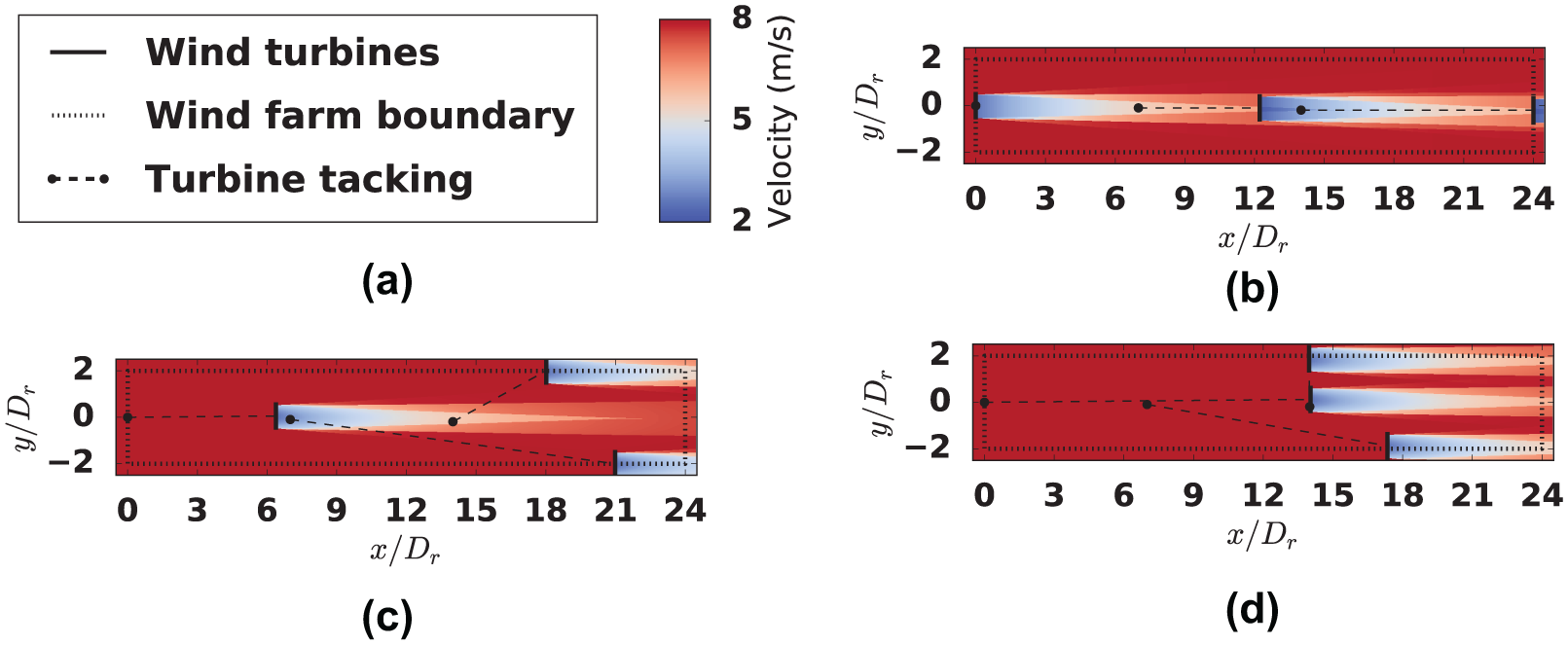
Unidirectional, position-only optimization for wind turbines starting in the center of the upstream turbines’ wakes as shown in Figure 9. Wind is from the left at 8 m/s. All figures share the legend and color bar. (a) Legend and color bar for (b-d). The color bar is equivalent to the color bar in Figure 9(b). (b) Wind farm from Figure 9(a) optimized with the original FLORIS model using finite differences for gradient calculations. Visualized with the original FLORIS model. (c) Wind farm from Figure 9(a) optimized with the cosine version of the FLORIS model using finite differences for gradient calculations. Visualized with the cosine version of the FLORIS model. (d) Wind farm from Figure 9(a) optimized with the cosine version of the FLORIS model using exact gradients. Visualized with the cosine version of the FLORIS model.
Case study 3: pseudo-random wind farm
Methods
Because the grid case study (case study 1: scaling) started close to a known local optimum, it may not be representative of differences in exploration and convergence. In this case study, we optimized a wind farm of 25 turbines with pseudo-random starting points as shown in Figure 11. We created the wind farm boundary from the convex hull of the initial positions. Yaw was initialized to zero. In this case study, AEP was maximized with respect to position and yaw using the wind data shown in Figure 7. The optimization problem was formulated as
The normal distance from each turbine to each boundary (
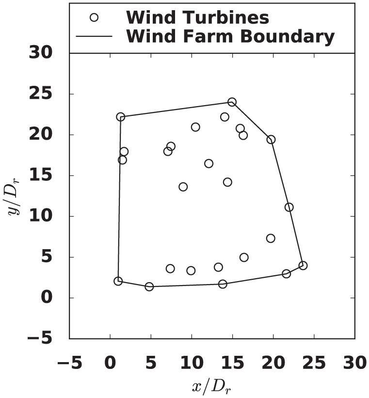
Pseudo-random wind farm starting locations and fixed boundary. Circle diameter is rotor diameter.
Results and discussion
Figure 12 shows a large increase in convergence rate when using exact gradients. It also demonstrates that the cosine term may help the optimization converge with slightly fewer function calls, even when finite-difference gradients are used. Because of the 1775 design variables, variants using finite differences required more function calls per iteration than those using exact gradients required to converge on a final solution.
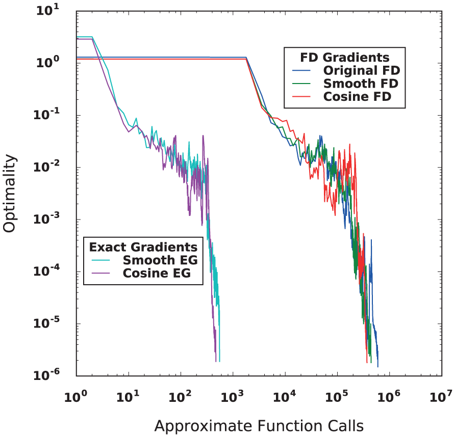
Progression of optimality (the norm of the Lagrangian) versus the approximate number of function calls during optimization in case study 3 for variants of the FLORIS model.
Conclusion
The changes to the FLORIS model presented in this work were shown to increase the compatibility of the FLORIS model for use with gradient-based optimization as compared with the original FLORIS model. Using exact gradients reduced the number of function calls required by two to three orders of magnitude. The added curvature, included via a simple cosine term, decreased the probability of premature convergence. Future work should include investigating multistart approaches using gradient-free methods to determine several starting points and then optimizing with gradient-based methods using exact gradients. Future work should also investigate the speedup potential for optimizing with exact gradients and address ways to reduce the cost of combining the gradients of each sub-model to obtain the gradient of the objective function.
Footnotes
Appendix 1
Acknowledgements
The authors would like to thank the OpenMDAO development team and the staff of the Fulton Supercomputing Lab at Brigham Young University for their technical support on this project. Any opinions, findings, and conclusions or recommendations expressed in this material are those of the author(s) and do not necessarily reflect the views of the National Science Foundation.
Declaration of conflicting interests
The author(s) declared no potential conflicts of interest with respect to the research, authorship, and/or publication of this article.
Funding
The author(s) disclosed receipt of the following financial support for the research, authorship, and/or publication of this article: This journal article was developed based, in part, on funding from the Alliance for Sustainable Energy, LLC, Managing and Operating Contractor for the National Renewable Energy Laboratory for the US Department of Energy. The BYU authors’ work was partially supported by the National Science Foundation under Grant No. 1539384.