Using TurbSim stochastic simulator to improve accuracy of computational modelling of wind in the built environment

Abstract

Small wind turbines are often sited in more complex environments than in open terrain. These sites include locations near buildings, trees and other obstacles, and in such situations, the wind is normally highly three-dimensional, turbulent, unstable and weak. There is a need to understand the turbulent flow conditions for a small wind turbine in the built environment. This knowledge is crucial for input into the design process of a small wind turbine to accurately predict blade fatigue loads and lifetime and to ensure that it operates safely with a performance that is optimized for the environment. Computational fluid dynamics is a useful method to provide predictions of local wind flow patterns and to investigate turbulent flow conditions at small wind turbine sites, in a manner that requires less time and investment than actual measurements. This article presents the results of combining a computational fluid dynamics package (ANSYS CFX software) with a stochastic simulator (TurbSim) as an approach to investigate the turbulent flow conditions on the rooftop of a building where small wind turbines are sited. The findings of this article suggest that the combination of a computational fluid dynamics package with the TurbSim stochastic simulator is a promising tool to assess turbulent flow conditions for small wind turbines on the roof of buildings. In particular, in the prevailing wind direction, the results show a significant gain in accuracy in using TurbSim to generate wind speed and turbulence kinetic energy profiles for the inlet of the computational fluid dynamics domain rather than using a logarithmic wind-speed profile and a pre-set value of turbulence intensity in the computational fluid dynamics code. The results also show that small wind turbine installers should erect turbines in the middle of the roof of the building and avoid the edges of the roof as well as areas on the roof close to the windward and leeward walls of the building in the prevailing wind direction.

Keywords

Small wind turbines built environment computational fluid dynamics turbulence stochastic simulator TurbSim turbulence intensity

Introduction

The trend of distributed wind systems to be used on-grid is increasing, driven by economic factors such as high electricity prices as well as political and social factors including a desire to combat climate change and to be energy independent. In 2005, 14% of small and medium wind systems in the United Kingdom were used on-grid, while in 2011, the percentage had increased to 45% (RenewableUK, 2012). Changing from off-grid to on-grid sites means the distributed wind system is often sited in the built environment. The installation can vary from small wind systems used on the rooftops of buildings, in car parks, along the side of freeways, and so on, to medium wind systems used in industrial sites or even large wind turbines used on university campuses.

The installation of small wind turbines (SWTs) in the built environment poses some challenges to be overcome, including the energy yield reduction resulting from lower mean wind speeds in urban areas as well as environmental impacts (Stankovic et al., 2009). In addition, the built environment is a much more complex environment than the open terrain sites assumed in the international SWT design standard IEC61400-2 (Tabrizi et al., 2014). Sites can include locations near buildings, trees and other obstacles, and in such locations, the wind is normally highly three-dimensional (3D), turbulent, unstable and at times weak (Makkawi et al., 2009), and some sites may experience values of inflow turbulence intensity (TI) that are many times greater than an open field site. Knowledge about flow conditions play a particularly important role for these sites since the level of turbulence significantly affects the power output of the turbine, and elevated TI has been found to be the most important factor in reducing turbine life from fatigue life (Riziotis and Voutsinas, 2000). There have been some very public failures of SWTs in the built environment due to misunderstanding turbulent flow conditions, notably in situations where the turbines have been mounted on top of the buildings (Fontsocial, 2012; Gipe, 2014; Bergey Windpower, 2009). Recent research by the International Energy Agency (IEA) Wind RD&D Task 27 has indicated that the turbulence design thresholds in the current international standard for SWTs, IEC 61400-2:2011 (2011, ed. 3) are too low for SWTs in urban wind sites, and a better characterization of turbulence is required for these kind of highly turbulent sites.

For large wind turbine sites, performing a comprehensive assessment of the wind resource yields knowledge about the characteristics of the level of the wind at the site as well as parameters related to turbulence. Turbulence is an important parameter to factor into wind turbine design, as it causes cyclic loading on the blades and can lead to blade fatigue. In understanding the inflow to an SWT in the built environment, a resource assessment of the potential wind site can also be used to determine the wind characteristics, including the turbulence levels that the SWT will experience. Small-scale rooftop urban projects compared to utility-scale or community-scale wind projects, do not typically have access to large amounts of fiscal resources for the resource assessment phase of a project and thus investment in measurement equipment is usually limited. In addition, for urban environments, the traditional methods for wind energy site assessment are technically limited; the complex geometry can result in situations where the resource varies substantially within a small area, thus a single meteorological mast may not be a sufficiently good indicator of the overall resource within a complex environment. Also, remote sensing technologies such as wind-detecting LiDAR are typically designed to work at 40 m or above and many small-scale rooftop urban projects are designed for deployment at lower heights.

Computational fluid dynamics (CFD) techniques can be a reliable alternative for a less expensive and faster method to predict turbulent flow conditions for a small rooftop wind turbine (Kalmikov et al., 2010). Heath et al. (2007) modelled the flow characteristics within an urban area over an array of pitched-roof houses using CFD. In this work, CFD modelling was used to compute mean wind speeds at potential turbine-mounting points and identify optimum mounting points for different prevailing wind directions in terms of maximum power availability. A numerical study of wind flow above the roof in three suburban landscapes with houses with the three different roof shapes of pitched, pyramidal and flat roofs has been performed by Ledo et al. (2011). They used a CFD technique to simulate the wind flow and investigate the TI and turbulence kinetic energy (TKE) over three different roof shapes. Their results show that the wind flow characteristics are strongly dependent on the shape of the roofs, with turbines mounted on flat roofs likely to generate higher and more reliable power for the same turbine hub elevation than the other roof profiles. Kalmikov et al. (2010) assessed the wind energy potential on the campus of the Massachusetts Institute of Technology in Cambridge, MA, using CFD simulation. They integrated local wind measurements and observations from some nearby reference sites into the CFD model to estimate the local long-term climatology to enhance the evaluation. Comparisons of measurements with simulated results provided validation of the model for mean wind-speed TI, wind power density, and wind variability parameterized by a Weibull distribution. Their work resulted in a better understanding of the micro-climate of the wind resource on the MIT campus and was used to determine the optimal siting of a small turbine on campus.

These examples illustrate the potential for using CFD as a valuable resource assessment tool. A local municipality, for instance, may be interested in using such a tool together with information from a regional wind atlas to provide insight into the feasibility of roof-mounted wind turbines within their boundaries. The results of CFD modelling, however, are sensitive to the choice of input values to the model. Accurate CFD results are critically dependent on having realistic values at the inlet of the CFD domain. Using incorrect inlet values leads to inaccurate output results or simulations which do not converge. Most CFD packages provide different options for setting inlet values; for example, in terms of inlet values for turbulence, it is possible to use either a percentage value of TI, or input TI or TKE profiles to the inlet of the domain. The first option is the simplest, whereas the latter would require the user to have additional expertise in using other software to generate such profiles. Accurate TKE profiles for the target area would be the best representation of the turbulence at the inlet of the domain, but this article asks the research question: what gains in accuracy can be achieved by using TKE profiles compared to setting a percentage TI level, given that the user would need to invest in additional software and training to use the profiles approach?

In this research, the ANSYS CFX 14.5 CFD software package is used to simulate turbulent flow over a building (ANSYS Inc, 2014). Tabrizi et al. validated the CFX simulation of flow around obstacles by using secondary data from the CEDVAL wind tunnel datasets from Hamburg University. To assess the accuracy of CFX in simulating turbulence conditions around obstacles, a test case was performed to model the flow around a rectangular structure (Tabrizi et al., 2014). The simulation results were then compared with the well-known CEDVAL wind tunnel datasets from Hamburg University (Meteorologisches Institut of Hamburg University, 2014).

A CFD model of Bunning Group Ltd’s warehouse at Port Kennedy in Western Australia was developed using the TurbSim stochastic simulator to find the wind speed and TKE profiles at the inlet of the CFD domain (Kelley and Jonkman, 2007). The wind atlas software WAsP was then applied to predict the reference wind speeds as an input to the TurbSim stochastic simulator (DTU Wind Energy, 2014). This research is valuable as the CFD simulations are carried out on a building (the Bunnings warehouse), where there is an existing measurement system in place, allowing direct comparison between measurements and the model output.

The aim of this study is to investigate the application of the TurbSim stochastic simulator to improve the accuracy of computational modelling of wind in a built up environment in order to provide guidance in the micro-siting of SWTs in the built environment. The specific objectives to achieve this aim are:

To assess how the combination of the CFD package CFX and the TurbSim stochastic simulator can improve the accuracy of CFD results of wind simulation in the built environment.

To use the combination of CFX and TurbSim to investigate the effects of the complex urban topography on turbulence on the rooftop by identifying high and low turbulent zones. Identification of zones of high turbulence is important to protect the SWT from excessive loading caused by turbulence from nearby structures and then to avoid installation in those areas.

Methodology

To assess how the combination of a CFD package with the TurbSim stochastic simulator improves the results of the CFD simulation of the wind in the built environment, a CFD model of the Bunnings warehouse was created by means of CFX software. The buildings around the warehouse (up to 200 m radius) were added to the model domain. The built-up area surrounding the warehouse is shown in Figure 1. Then two different approaches were applied to predict the wind-speed profiles and turbulence levels at the inlet of the CFD domain. In the first approach, called the regular approach, WAsP was applied to predict the mean wind speeds at a reference height of 200 metres and a logarithmic wind shear profile was assumed in order to extrapolate these wind speeds down to the level of the heights of the CFD domain. In the regular approach, the turbulence level at the inlet boundary was adjusted by 5% as suggested in CFX guidelines (ANSYS Inc., 2012). This approach was applied by Tabrizi et al. (2014) to gain insight into inflow conditions over a rooftop with SWTs.

Figure 1.

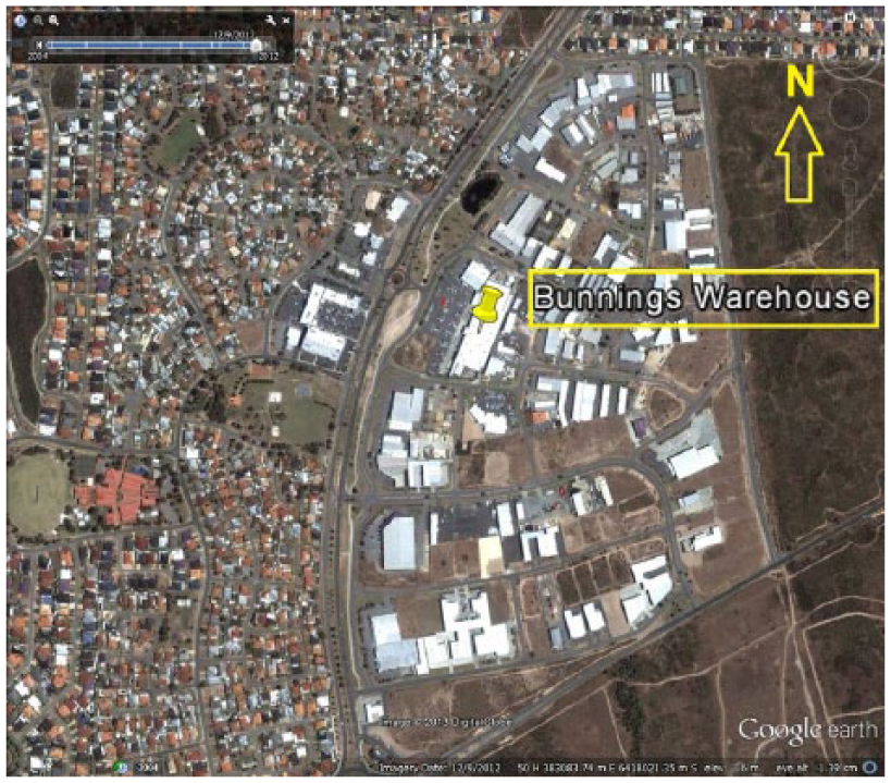
The built-up area surrounding the Bunnings warehouse in Port Kennedy, Western Australia.

To predict the mean wind speeds at a reference height, the wind atlas software WAsP was used. Raw data from the Kwinana Industries Council meteorological station located on Alcoa RDA Lake, taken between 12 August and 24 January for 4 years (2004–2007) were used as wind observations in WAsP. Figure 2(a) shows the location of the meteorological station compared to the location of the Bunnings warehouse, and Figure 2(b) shows the geometry and layout of the buildings around the Bunnings warehouse as well as the location of the anemometer on the warehouse.

Figure 2.

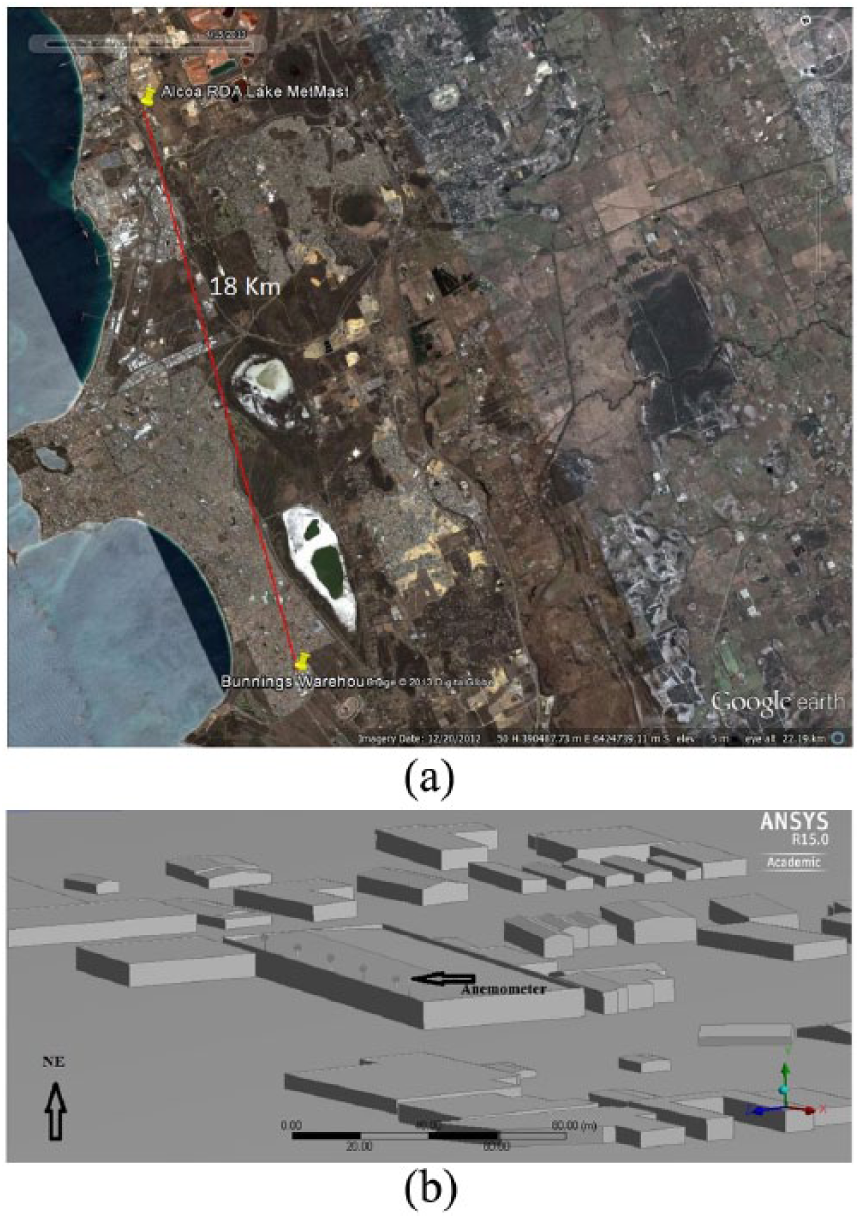
(a) Comparison of the locations of the Alcoa RDA Lake meteorological station and the Bunnings warehouse and (b) building geometry around the Bunnings warehouse building and the anemometer location.

The generalized wind atlas provided by WAsP was used to predict the wind shear profile by assuming a roughness value of the area far outside around the Bunnings warehouse (the area with radius bigger than 200 m around the Bunnings warehouse) that included mean wind speeds at 200 m above the ground in each of eight wind direction sectors N, NE, E, SE, S, SW, W, and NW. Since the characteristics of wind speed at 200 m above the ground are site independent, they were used to predict the logarithmic vertical wind profile, which was then used as the inlet velocity profile in the regular approach for the CFD model.

In the second approach, called TurbSim approach, the mean wind speeds at a reference height of 200 m from the WAsP simulations were used as the reference wind speeds in the TurbSim simulator to compute the vertical wind speed and TKE profiles. These profiles were then applied at the inlet of the CFD domain for each simulated wind sector. The model was run for similar each sector to find the wind speed on the roof of the warehouse. More information about the inlet wind speed and TKE profiles has been provided in the description of the CFD model in section ‘CFD model’. The results were extracted for the same dates as the actual ultrasonic measurements from the anemometer to allow for a comparison between simulation and measurement for both approaches. CFX assumes a neutral atmospheric stability and thus the CFD results have been compared with neutrally stable wind data measured on the roof of the Bunnings warehouse to check the accuracy of the combination of CFD and TurbSim stochastic simulator to assess the rooftop wind. To isolate the neutrally stable data, the wind measurements above the Bunnings rooftop are filtered by applying Golder’s (1972) curve of Pasquill stability classes as functions of the Monin–Obukhov length and roughness length. The European wind atlas was consulted, and the aerodynamic roughness of the area far outside around the Bunnings warehouse (the area with radius bigger than 200 m around the Bunnings warehouse) was estimated to be 50 cm (Troen and Petersen, 1989). Figure 3 shows the summary of both approaches.

Figure 3.

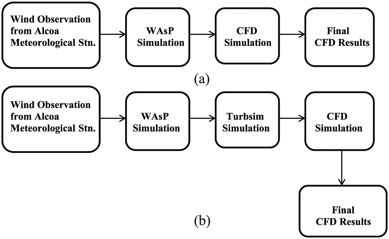
(a) CFD modelling methodology – regular approach and (b) CFD modelling methodology – TurbSim approach.

Site and measurement campaign

The warehouse is a rectangular building, with its long-axis oriented NNE-SSW, a façade wall around the edge of the roof that is 8.4 m above ground level and a very low pitched roof (almost flat). The building is approximately 5 km from the coast (Indian Ocean) with the prevailing winds are from the south-west. The warehouse is situated in a commercial district but has no larger buildings or trees in the vicinity. Within a 1 km radius of the site, there are mainly residential buildings to the north, commercial and industrial buildings to the west, and a few buildings, low shrubs, and low sand dunes to the south and east. The south-west front and the north-west side are comparatively open, though street furniture¹ and a car park exist on these sides (Hossain, 2012).

A wind-monitoring system was installed in September 2009 as part of a wind resource assessment for the installation of five SWTs that were later installed in March 2010. The Gill WindMaster Pro 3D ultrasonic anemometer was installed on a boom on a 5.3-m tall mast attached to the front-façade of the warehouse. The boom has a sliding collar in order to position the ultrasonic anemometer at different heights above the roof. The mast can be tilted down in order to make adjustments or to replace sensors. The data consist of 10 Hz data over a 6-month period (between 8 August 2011 and 24 January 2012). Figure 4 indicates the position of the ultrasonic anemometer on the roof.

Figure 4.

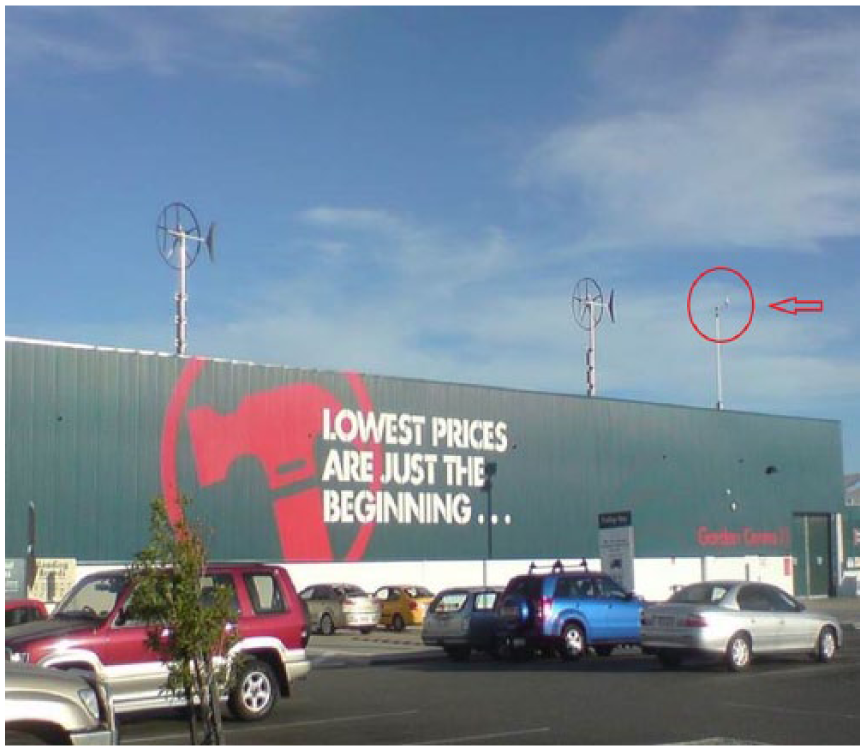
Position of the ultrasonic anemometer on the roof of the Bunnings warehouse.

TurbSim

TurbSim, developed by the US Department of Energy’s National Renewable Energy Laboratory (NREL) is a stochastic, full-field, turbulent-wind simulator. This simulator applies a statistical model to numerically simulate a time series of three-component wind-speed vectors at points on a fixed, two-dimensional (2D) vertical rectangular grid (Jonkman, 2009). Dynamic analysis software packages such as FAST (Jonkman and Buhl, 2005), YawDyn (Laino and Hansen, 2003) or MSC.ADAMS can use the output of TurbSim as input data, where Taylor’s frozen turbulence hypothesis has been utilized to obtain local wind speeds, interpolating the TurbSim-generated fields in both time and space (Jonkman, 2009).

The spectra of velocity components and spatial relationships are defined in the frequency domain, and a time series is produced by applying an inverse Fourier transformation. A stationary process has been assumed as the underlying theory behind this method of simulating the time series. Coherent turbulent structures can be superimposed onto the time series generated by TurbSim to simulate non-stationary components (Jonkman, 2009). TurbSim allows the user to select a turbulence spectra model from default models or apply a numerical user-defined turbulence spectra and produces a 3D wind flow field with wind fluctuations governed by the spectra model.

CFD model

Navier–Stokes equations and turbulence models

ANSYS CFX 14.5, developed by ANSYS Inc, USA, was used to perform the CFD simulations. The literature has many examples of using different methods in CFD simulations such as direct numerical simulation (DNS) (Takahashi et al., 2006); large eddy simulation (LES) (Tutar and Oğuz, 2004; Uchida and Ohya, 2008) or the Reynolds-averaged Navier–Stokes (RANS) method with various turbulence models (Menter, 1994; Sørensen, 1995). The flow details that need to be obtained and the available computing resources are two critical criteria for choosing a proper method. Usually, it suffices to use the well-established RANS equations when only quasi-steady data is of interest, and that approach has been taken in this study (Ledo et al., 2011).

For steady-state modelling of wind flowing over a complex terrain, the RANS approach combined with a k-epsilon $(k - ε)$ scheme as the turbulence model, is the most common approach in wind engineering. The method provides a reasonable compromise between computational costs and accuracy. Reynolds decomposition is employed on the variables of the governing equations (each of them is divided in a time-averaged part and a fluctuating part, $u = \bar{u} +$ ú) resulting in the two following equations (Tabrizi et al., 2014)

ρ (\frac{\partial {\bar{u}}_{i}}{\partial t} + {\bar{u}}_{j} \frac{\partial {\bar{u}}_{i}}{\partial x_{j}}) = - \frac{\partial \bar{P}}{\partial x_{i}} + ρ {\bar{g}}_{i} + \frac{\partial}{\partial x_{j}} [μ (\frac{\partial {\bar{u}}_{i}}{\partial x_{j}} + \frac{\partial {\bar{u}}_{j}}{\partial x_{i}})] - \frac{\partial}{\partial x_{j}} ρ \bar{_{i}_{j}}

(1)

\frac{\partial {\bar{u}}_{k}}{\partial x_{k}} = 0

(2)

τ_{i j} = - ρ \bar{ú_{i} ú_{j}} = μ_{t} (\frac{\partial u_{i}}{\partial x_{i}} + \frac{\partial u_{j}}{\partial x_{i}}) + \frac{2}{3} ρ k δ_{i j}

(3)

The ‘standard’ k-epsilon $(k - ε)$ model, based on a two-equation turbulence energy scheme provides reasonable accuracy in approximately neutral atmospheric conditions. This model also provides an acceptable estimate of the TI and TKE (Michelsen, 1992).

In this study, as suggested by CFX guidelines, the shear stress transport (SST) scheme was used as the turbulence model (ANSYS Inc., 2012). The SST scheme is a hybrid two-equation model that combines the advantages of both k-epsilon $(k - ε)$ and k-omega $(k - ω)$ models. The SST k-ω equations are

\frac{\partial ρ k}{\partial t} + \frac{\partial}{\partial x_{j}} (ρ U_{j} k) = \frac{\partial}{\partial x_{j}} [(μ + \frac{μ_{t}}{σ_{k_{3}}}) \frac{\partial k}{\partial x_{j}}] + P_{k} - β^{'} ρ k ω + P_{k b}

(4)

\frac{\partial ρ ω}{\partial t} + \frac{\partial ρ ω}{\partial x_{j}} (ρ U_{j} k) = \frac{\partial}{\partial x_{j}} [(μ + \frac{μ_{t}}{σ_{ω_{3}}}) \frac{\partial ω}{\partial x_{j}}] + (1 - F_{1}) 2 ρ \frac{1}{ω σ_{ω_{2}}} \frac{\partial k}{\partial x_{j}} \frac{\partial ω}{\partial x_{j}} - α_{3} \frac{ω}{k} P_{k} - β_{3} ρ ω^{2} + P_{w b}

(5)

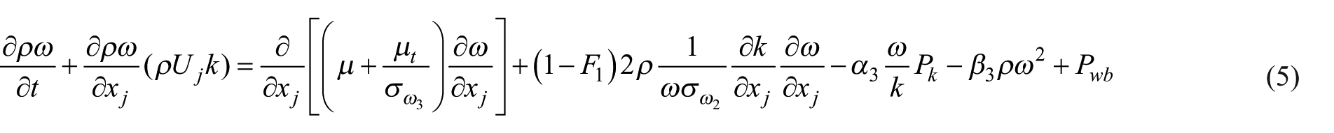
The SST model incorporates transport effects in the formulation of the eddy-viscosity and thus pays more attention to the transport of TKE and predicts the starting of and the size of the separation of flow under adverse pressure gradients more accurately than the standard $(k - ε)$ model. This leads to an improvement in the prediction of flow separation, which is required in this study to investigate turbulence (Ledo et al., 2011).

Inlet wind speed and TKE profiles

As mentioned in section ‘Methodology’, to assess how the combination of a CFD package with the TurbSim stochastic simulator influences the results of wind CFD simulation in the built environment, two different approaches were applied to predict wind-speed profile and turbulence level at the inlet of the CFD domain. In the regular approach, the following equation was used to model the wind profile at the inlet of CFD domain as suggested by Tabrizi et al. (2014)

u = \frac{u_{*}}{k} \ln (\frac{z + z_{0}}{z_{0}})

(6)

Since all the buildings within a radius of 200 m around the target building were simulated in the CFD model and the proper values for roughness of the ground, walls, and roofs of the buildings (2 cm) were applied in the CFD model. Therefore, to avoid duplication of the effects of roughness, the value of $z_{0}$ at equation (6) was set to 10⁻²⁰ m (the minimum acceptable value in CFX) for all eight wind sector simulations (the roughness effect of the obstacles at the area with radius bigger than 200 m around the Bunnings warehouse already has been taken to account in WAsP simulation). For each simulated wind sector, the mean wind speed 200 m above the ground (the output of the WAsP simulations) was used to find the friction velocity for the CFD simulation. Table 1 shows the results of the WAsP simulations in terms of mean wind speed for each sector (Tabrizi et al., 2014). Also, in the regular approach, the turbulence level at the inlet boundary was adjusted by 5% as suggested by CFX guidelines (ANSYS Inc., 2012).

Table 1.

WAsP output: sector-wise mean wind speeds at 200 m.

Wind sector	Mean wind speed (m/s)
North	6.36
North-East	5.33
East	8.01
South-East	7.57
South	8.53
South-West	8.36
West	6.19
North-West	6.18

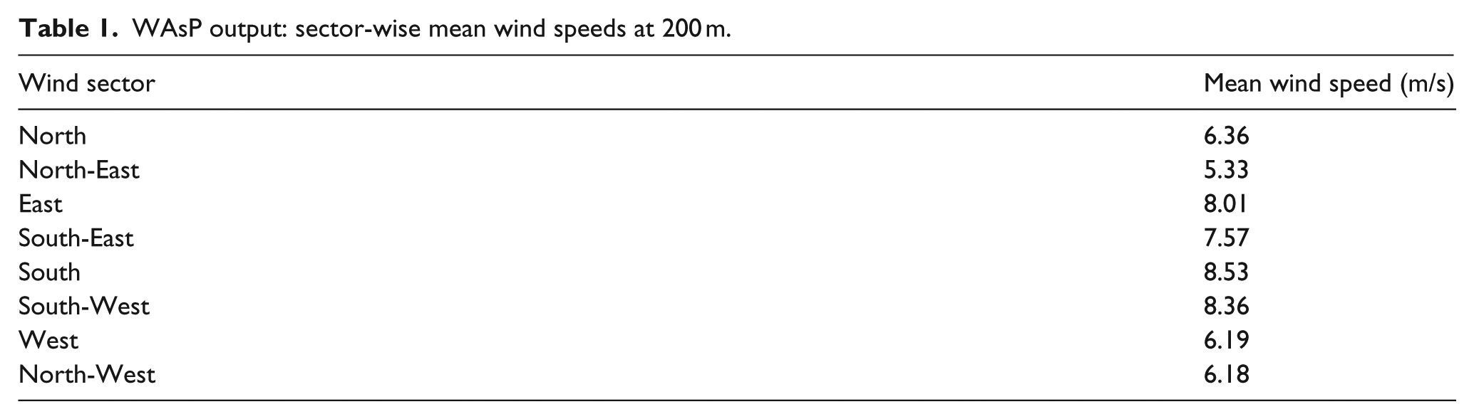
In the TurbSim approach, the TurbSim stochastic simulator was used to produce an accurate profile of wind speed and TKE at the inlet of CFD domain. The values from Table 1 were applied as inputs to TurbSim to represent reference velocities 200 m above the ground for each simulated wind sector. Several different spectral models are available in TurbSim, including two IEC models, the Risø smooth-terrain model, and several NREL site-specific models (Jonkman, 2009). To investigate the accuracy of the spectral models in simulating turbulence in the built environment, a 10-min TurbSim simulation was run using each of the available spectral models to yield the wind speed and TKE values at the height of the measurement zone of the ultrasonic anemometer on the rooftop of the Bunnings warehouse. The results of these runs showed that the IEC Kaimal model (defined in IEC 61400-1and IEC 61400-2:2006 (2006; Jonkman, 2009) calculated the values closest to the measured data for all simulated wind sectors. Therefore, the IEC Kaimal model was used in this study to provide the inlet wind speed and the TKE profiles.

To predict the wind speed and TKE profiles at the inlet of the CFD domain, the TurbSim stochastic simulator was run to find the values of wind speed and TKE at 28 different heights (between 1 and 15 m every 3 m and then between 15 and 125 m every 5 m) for each simulated wind sector. All the buildings within a radius of 200 m around the target building were simulated in the CFD model and the proper values for roughness of the ground, walls, and roofs of the buildings (2 cm) were applied in the CFD model (the roughness effect of the obstacles at the area with radius bigger than 200 m around the Bunnings warehouse already has been taken to account in WAsP simulation). Therefore, to avoid duplication of the effects of roughness, the TurbSim simulations assumed a perfectly smooth ground surface (the surface roughness length was set to 10⁻³⁶ m – the minimum acceptable roughness length in TurbSim). The IEC Kaimal model was chosen to model the turbulence power spectral density. The wind speed and TKE profiles were then produced for each wind sector by fitting a curve to the 28 wind speed and TKE values generated by TurbSim at the different heights for each sector.

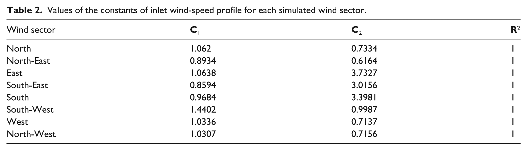
Using the curve-fitting procedure from TurbSim on the output data, the general profile of wind speed at the inlet of the CFD domain for all sectors is given by equation (7), where the values for the constants are shown in Table 2. When the 28 points were used, the value for the coefficient of determination, R² of the fitted curve was one

u = C_{1} \ln (z) + C_{2}

(7)

where $z$ is the height (m).

Table 2.

Values of the constants of inlet wind-speed profile for each simulated wind sector.

Wind sector	C ₁	C ₂	R ²
North	1.062	0.7334	1
North-East	0.8934	0.6164	1
East	1.0638	3.7327	1
South-East	0.8594	3.0156	1
South	0.9684	3.3981	1
South-West	1.4402	0.9987	1
West	1.0336	0.7137	1
North-West	1.0307	0.7156	1

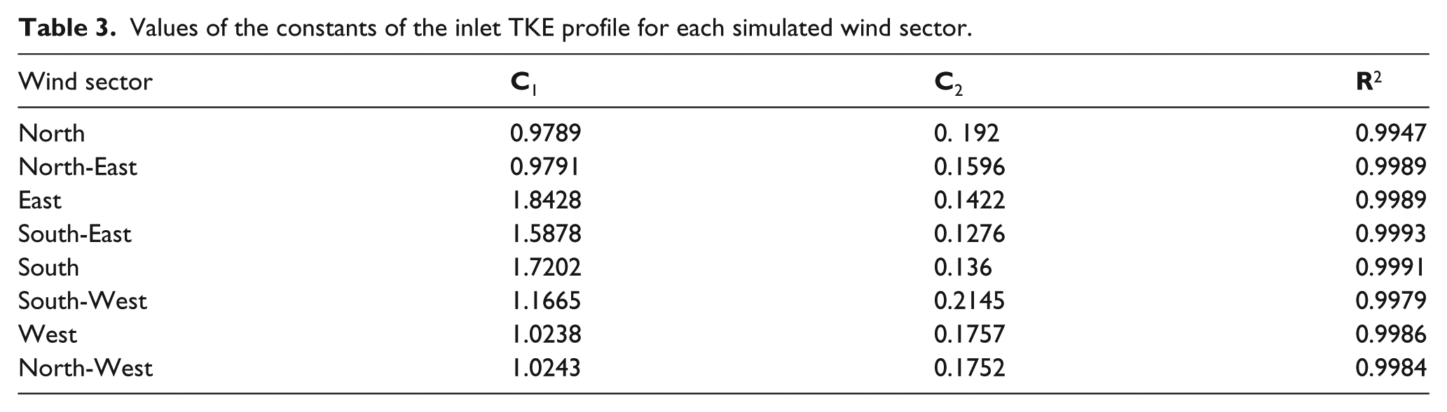
Using the curve-fitting procedure from TurbSim on the output data, the general profile of the TKE at the inlet of the CFD domain for all sectors is given by equation (8), where the values for the constants are shown in Table 3. When the 28 points were used the value for the coefficient of determination, R² of the fitted curve was very close to one

T K E = C_{1} {(z)}^{C_{2}}

(8)

where $z$ is height (m).

Table 3.

Values of the constants of the inlet TKE profile for each simulated wind sector.

Wind sector	C ₁	C ₂	R ²
North	0.9789	0. 192	0.9947
North-East	0.9791	0.1596	0.9989
East	1.8428	0.1422	0.9989
South-East	1.5878	0.1276	0.9993
South	1.7202	0.136	0.9991
South-West	1.1665	0.2145	0.9979
West	1.0238	0.1757	0.9986
North-West	1.0243	0.1752	0.9984

Inlet epsilon (turbulence eddy dissipation) profile

In the TurbSim approach, CFX also requires information on the turbulence eddy dissipation, $ε$ at the inlet of the CFD domain. The turbulence eddy dissipation inlet profile can be specified in terms of the following equation (Martinez, 2011):

ε = \frac{T K E^{1.5} C_{μ}^{0.75}}{l}

(9)

In the IEC 61400-2:2011 (2011) standard, the longitudinal integral length scale has been suggested as 5.67z, where z is the height (m) from the ground. The same formulation is applied for the integral length scale (l) in equation (9).

Computational mesh

An unstructured tetrahedral mesh was used with 20 layers increasing in thickness as they get further from the surface (first layer thickness of 1 mm) on the ground as well as on the roofs and walls of all buildings in all of the wind sector modelling. The mesh is refined at the ground, roofs and walls of all buildings to define the boundary layer. The grid is concentrated near the fixed surfaces, and the measured y+ is in the range of 30–300 mm. As the grid moves further away from the surfaces, it is enlarged by an expansion ratio of 1.2. The number of mesh elements was around 2.5 million for each simulated sector.

Boundary domain, boundary conditions and initial conditions

For all wind sectors, the simulated buildings were placed in a rectangular domain whose height is equal to 16H_max, where H_max is the height of the highest simulated building in the region of interest (H_max = 8.5 m). The lateral boundaries of the computational domain were placed at a distance of 5H_max away from the closest part of the built up area at each side. A distance of 8H_max between the inflow boundary and the built up area was applied as the longitudinal extension of the domain in front of the simulated region, and a distance of 15H_max behind the built up area was employed to allow for flow re-development. The TKE, turbulence eddy dissipation, velocity and pressure values were set to default values as initial conditions (Tabrizi et al., 2014).

The downstream boundary was specified as an outlet with a neutral relative pressure and a neutral TI gradient. Symmetric boundary conditions were employed for the sides and top of the domain in all wind sectors. Solid boundaries including the ground of the domain and roofs and walls of the buildings were set as no-slip walls with the CFX wall-function approach used to model flow near these surfaces (Martinez, 2011). An automatic near-wall treatment method was used in CFX to treat the wall effects. The near-wall treatment method accounts for the rapid variation of flow variables that occur within the boundary layer region as well as viscous effects at the wall. This treatment provides a smooth shift from low-Reynolds number formulations to the wall-function formulation (Tabrizi et al., 2014).

Results and discussion

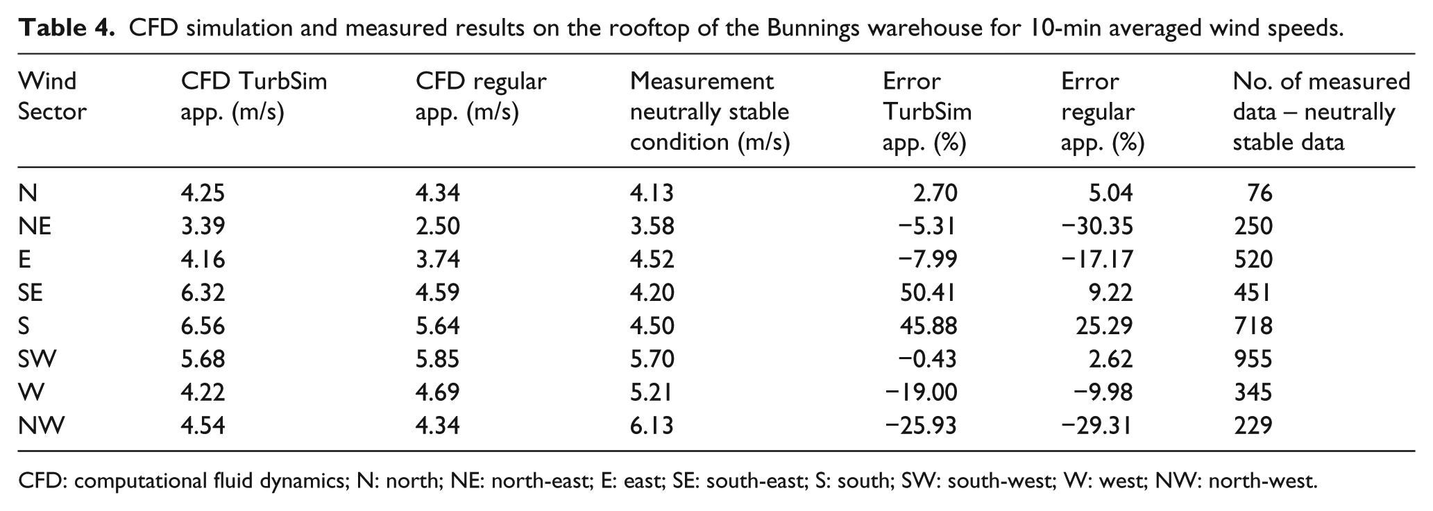
Table 4 shows the CFD simulated and measured results for the 10-min averaged 3D velocity vectors on the rooftop of the Bunnings warehouse building. The results cover a period between 12 August 2011 and 24 January 2012, under neutral and stable atmospheric conditions. The curves presented by Golder (1972) were used to find the range of Monin–Obukhov lengths corresponding to the neutrally stable condition on the roof of the warehouse for a 10 min averaging period and these values were used to filter the raw measurements. The percentage of error between the numerical results and the measured results are presented in the table for all wind sectors. The CFD results of both approaches have been included in the table.

Table 4.

CFD simulation and measured results on the rooftop of the Bunnings warehouse for 10-min averaged wind speeds.

Wind Sector	CFD TurbSim app. (m/s)	CFD regular app. (m/s)	Measurement neutrally stable condition (m/s)	Error TurbSim app. (%)	Error regular app. (%)	No. of measured data – neutrally stable data
N	4.25	4.34	4.13	2.70	5.04	76
NE	3.39	2.50	3.58	−5.31	−30.35	250
E	4.16	3.74	4.52	−7.99	−17.17	520
SE	6.32	4.59	4.20	50.41	9.22	451
S	6.56	5.64	4.50	45.88	25.29	718
SW	5.68	5.85	5.70	−0.43	2.62	955
W	4.22	4.69	5.21	−19.00	−9.98	345
NW	4.54	4.34	6.13	−25.93	−29.31	229

CFD: computational fluid dynamics; N: north; NE: north-east; E: east; SE: south-east; S: south; SW: south-west; W: west; NW: north-west.

Results for north, north-east, east, south-west and north-west sectors with the TurbSim approach were better compared to the regular approach. TurbSim provided a particularly accurate CFD result when the prevailing wind direction was from the south-west sector (0.43% error). However, for the north-west and the west sectors the TurbSim approaches were poor (25.93% and 19% error). The discrepancy in results from these sectors may be due to a combination of lack of measured data from those sectors and the effect of some high light towers around the building. These factors clearly cause some disturbance in the north-west sector not included in the CFD model. The TurbSim approach provided very poor results for the south-east and the south sectors (50.41% and 45.88% error). This could be attributed to the fact that when the wind comes from the south-east and south sectors, the measurement point may be located inside a recirculation zone. TurbSim was originally developed for open terrain applications and the inlet values cannot provide accurate outcomes for flows inside a recirculation zone. It is also likely that the turbulence models used for CFD simulation did not work well inside a recirculation zone. Wind flows that come from the south and south-east directions may separate at the edge of the top of the façade on the south facing wall of the warehouse. The separation creates a boundary layer that increases with distance and contains recirculating flow. The anemometer height may be within the height of this boundary layer. In comparison, the distance of the anemometer from the top of the façade for other wind directions, for example, south-west may not be sufficient for the height of the boundary layer to be comparable with the height of the anemometer or may be sufficiently large to enable flow mixing to break up the recirculating zones.

Further work is needed to investigate the accuracy of different turbulence models inside the recirculation zone. The application of a more accurate turbulence model would likely improve the results for these sectors. However, from a practical point of view, recirculation zones should be avoided in terms of the application of SWTs on the rooftops of building. Installation of small machines in recirculation zones would make the machines vulnerable to higher turbulent inflow and higher loads and would likely lead to a shorter lifetime. As TurbSim has provided results with lower error for all the unobstructed sectors, it is a promising approach to improve the accuracy of wind resource assessments for SWTs on rooftops.

TI

To address the second research objective of this article, CFD is used to produce contour plots of TI over the building to identify areas of high turbulence that a SWT installer should avoid to ensure that the turbine does not experience excessive loading.

TI is defined as

T I = \frac{σ}{U}

(10)

where

σ = \sqrt{\frac{2}{3} (T K E)}

(11)

In designing an SWT in accordance with IEC Standard IEC 61400-2:2006 (2006), manufacturers assume that the wind turbine will not experience TI values greater than 18%. Estimating of TI at any prospective location prior to turbine installation is important as TI values higher than 18% are likely to affect the operation and the life of the turbine.

Figures 5 and 6 show some examples of the output from CFX for the case of winds from the south-west sector, the prevailing wind direction, by applying the TurbSim approach. Figure 5 shows the TI contours on the long west-facing edge of the building where the turbines and ultrasonic anemometer are installed; Figure 6 presents the TI contours on the middle of the roof along the NNE-SSW long-axis of the Bunnings warehouse. Comparison of Figures 5 and 6 shows that the value of TI is greater on the edge than in the middle of the roof. For most of the edge, the value of TI is around 30%, while the value is around 25% for most of the middle of the roof, and in both cases the value is higher than the 18% limit in the standard. Also, in both figures, the area on the roof immediately downwind of the windward-facing walls experienced the maximum value of TI on the roof (around 50%). Figures 5(a) and (c) also show very high values of TI on the roof immediately upwind of the leeward side of the building. The area on the leeward side of the building is characterized by high TI values due to recirculating flow behind the building.

Figure 5.

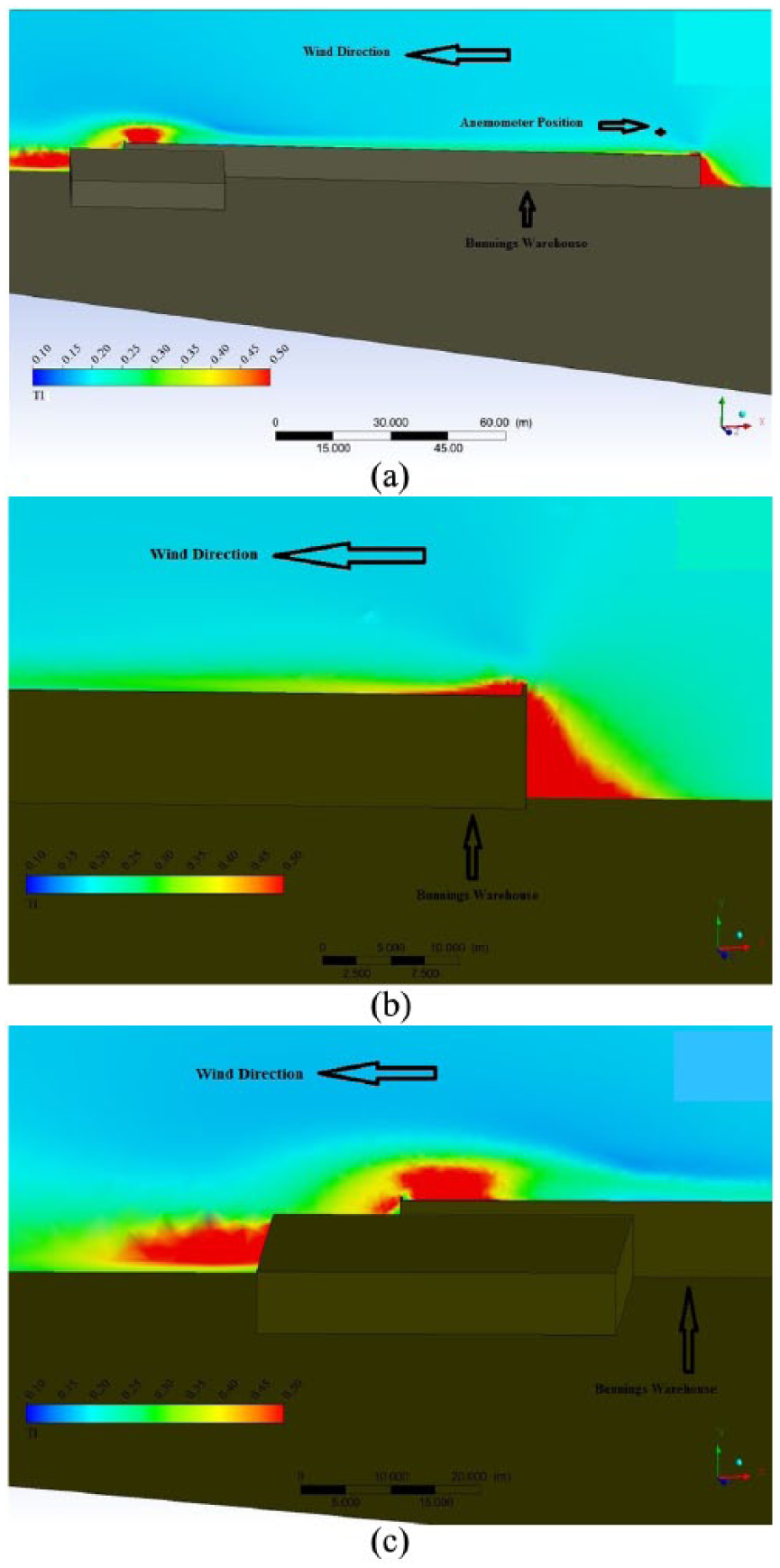
(a) TI contours in the edge of the roof of the Bunnings warehouse building for the south-west wind sector simulation, (b) close up of TI contours in the edge of the roof at the upwind side of the Bunnings warehouse building for the south-west wind sector simulation and (c) close up of TI contours in the edge of the roof at the downwind side of the Bunnings warehouse building for the south-west wind sector simulation.

Figure 6.

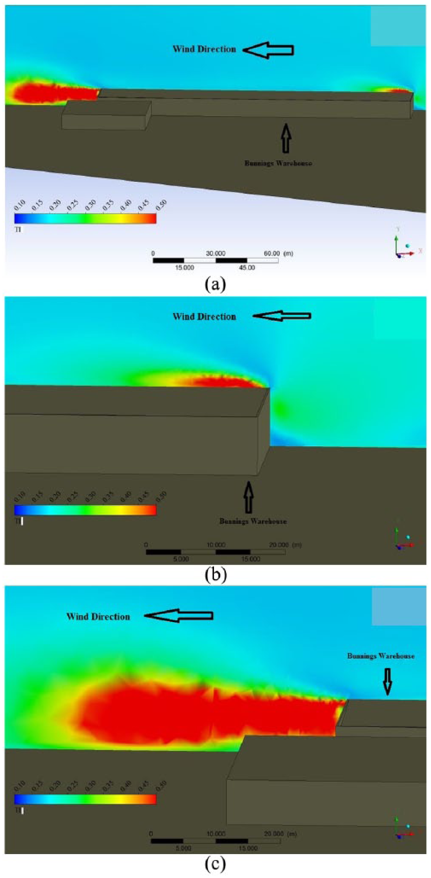
(a) TI contours along the centreline of the roof of the Bunnings warehouse building for the south-west wind sector simulation, (b) close up of TI contours along the centreline of the roof at the upwind side of the Bunnings warehouse building for the south-west wind sector simulation and (c) close up of TI contours along the centreline of the roof at the downwind side of the Bunnings warehouse building for the south-west wind sector simulation.

These types of figures can play an important role in micro-siting SWTs in the built environment. The range of values of TI can have a significant effect on SWTs fatigue loading. The areas with low TI values on the roof are the most desirable sites for installation, as they avoid high fatigue loads on the turbine. The figures suggest that the ideal location for installation of an SWT is in the middle of the roof of the Bunnings warehouse, away from the windward-facing walls of the building. In this location, the SWT will experience lower turbulence, lower loads and is likely to have a longer lifetime.

Before drawing conclusions from this research, the limitations of the study must be noted. First, only a few months of measured data were obtained (August 2011–January 2012) covering only the spring and summer seasons in the southern hemisphere. A year-long period of measured data on the rooftop would be preferable in order to consider any seasonal effects. In addition, for the WAsP simulation, the reference data have been taken from a meteorological station 18 km away from the target building. This study has assumed that the reference and target site have the same underlying regional wind climate. For the TurbSim simulation, the IEC Kaimal spectral model was found to be the best choice of available models but is also limited in its applicability. The Kaimal model assumes open terrain and the length scales of turbulence used in the model may not be appropriate for the built environment. This is supported by the research findings as the simulations have the greatest agreement for wind sectors where there are fewer obstacles and the poorest agreement for winds encountering the Bunnings building before being recorded by the ultrasonic anemometer.

Conclusion

A method to try and improve the accuracy of the CFD results for wind simulation over rooftop of a building in the built environment by using the TurbSim stochastic simulator was investigated. TurbSim was applied to predict the wind speed and TKE profiles at the inlet of the CFD domain. A CFD model of the Bunnings warehouse at Port Kennedy in Western Australia was created by means of the ANSYS CFX 14.5 package and the buildings around the warehouse up to a radius of 200 m were added in the model geometry. The mean wind speeds at a reference height of 200 m from the WAsP simulations were used as reference wind speeds in the TurbSim simulator. Observations for WAsP were taken from a metrological mast located 18 km from the Bunnings warehouse. A wind-monitoring system installed on the roof of the Bunnings warehouse at Port Kennedy was used to collect data for comparison with the CFD simulations. The TurbSim approach was used to investigate the turbulence conditions on the rooftop of a building and to identify the optimal location for installing SWTs on the roof, by locating zones of low TI.

For the prevailing wind direction at the building site, the TurbSim approach provided a very accurate CFD result by predicting averaged wind speeds. In general, the TurbSim approach provided better results in simulating the wind velocity for unobstructed sectors (where there is no flow blockage influencing the wind speed at the measurement point) compared to the regular approach (in the regular approach, the general logarithmic profile was used as the inlet wind-speed profile, and the turbulence level at the inlet boundary was adjusted by 5%). As SWTs should be sited outside of the recirculation zones due to flow blockage on the roof, the TurbSim approach is a promising approach to improve the accuracy for rooftop SWT wind resource assessment. However, further research into different turbulence models should be performed to investigate ways to improve the CFD results of wind simulation on rooftops for those sectors where the flow is obstructed, and there is turbulent flow affecting the measurement site.

The combination of CFX and TurbSim was also used to identify zones of high and low TI along the roof. Avoiding siting in high TI areas and installations in low TI areas would protect the turbine from excessive loading due to turbulence from neighbouring structures. The results show that SWT installers should erect the turbines in the middle of the roof of the building and avoid the edges of the roof as well as areas on the roof close to the windward and leeward walls of the building in the prevailing wind direction.

Accurate prediction of the turbulent flow conditions to an SWT on the rooftop is very important, since turbulence is linked to fatigue on the machine. Further research needs to be performed to study the effect of turbulence on the loading, fatigue, and generated power by SWTs on the rooftop of a building.

Footnotes

Appendix 1 Declaration of conflicting interests

The author(s) declared no potential conflicts of interest with respect to the research, authorship and/or publication of this article.

Funding

The author(s) received no financial support for the research, authorship and/or publication of this article.

Notes

ORCID iD

Amir Bashirzadeh Tabrizi

References

ANSYS Inc. (2012) ANSYS CFX-Solver Theory Guide Release 14.5. Canonsburg, PA: ANSYS Inc.

ANSYS Inc. (2014) Computational fluid dynamics (CFD) software. Available at: https://www.ansys.com/products/fluids

Bergey Windpower (2009) Warwick trials of building mounted turbines. Available at: http://www.bergey.com/technical/warwick-trials-of-building-mounted-wind-turbines

DTU Wind Energy (2014) WAsP – The wind atlas analysis and application program. Available at: http://www.wasp.dk

Fontsocial (2012) Case study: Wind turbines communications. Available at: https://www.fontpr.com.au/how/case-study-wind-turbines-communications/

Gipe

(2014) Wind-works. Available at: http://www.wind-works.org/cms/

Golder

(1972) Relations among stability parameters in the surface layer. Boundary: Layer Meteorology 3: 47–58.

Heath

Walshe

Watson

(2007) Estimating the potential yield of small building-mounted wind turbines. Wind Energy 10: 271–287.

Hossain

. (2012) Investigating Whether the Turbulence Model from Existing Small Wind Turbine Standards is Valid for Rooftop Sites. Perth, WA: School of Engineering and Energy, Murdoch University.

10.

IEC 61400-2:2006 (2006) Wind turbines – Part2: Design requirements for small wind turbines (2nd edn).

11.

IEC 61400-2:2011 (2011) Wind turbines – Part 2: Design requirements for small wind turbines (3rd edn).

12.

Jonkman

. (2009) TurbSim User’s Guide: Version 1.50. Boulder, CO: NREL.

13.

Jonkman

Buhl

MLJ

(2005) FAST User’s Guide. Boulder, CO: NREL.

14.

Kalmikov

Dupont

Dykes

et al . (2010) Wind power resource assessment in complex urban environments: MIT campus case-study using CFD analysis. In: Proceedings of the AWEA 2010 WINDPOWER conference, Dallas, TX, 23–26 May.

15.

Kelley

Jonkman

(2007) Overview of the Turbsim Stochastic Inflow Turbulence Simulator. Boulder, CO: NREL.

16.

Laino

Hansen

(2003) User’s Guide to the Wind Turbine Dynamics Computer Program YawDyn. Salt Lake City, UT: Windward Engineering LC.

17.

Ledo

Kosasih

Cooper

(2011) Roof mounting site analysis for micro-wind turbines. Renewable Energy 36: 1379–1391.

18.

Makkawi

Celik

Muneer

(2009) Evaluation of micro-wind turbine aerodynamics, wind speed, sampling interval and its spatial variation. Building Services Engineering Research and Technology 30: 7–14.

19.

Martinez

. (2011) Wind Resource in Complex Terrain with OpenFOAM. Risø DTU (Technical University of Denmark). Available at: https://www.yumpu.com/en/document/view/12401522/martinez-b-wind-resource-in-complex-terrain-with-openfoam

20.

Menter

. (1994) Two-equation eddy-viscosity turbulence models for engineering applications. AIAA Journal 32: 1598–1605.

21.

Meteorologisches Institut of Hamburg University (2014) CEDVAL wind tunnel datasets. Available at: http://mi-pub.cen.uni-hamburg.de/index.php?id=433

22.

Michelsen

. (1992) Basis3D – A Platform for Development of Multi-Block PDE Solvers. Lyngby: Technical University of Denmark.

23.

RenewableUK (2012) Small and medium wind UK market report. Available at: http://www.klein-windkraftanlagen.com/wp-content/uploads/2012/05/2012-0_RenewableUK_SMWMarketReport2012.pdf

24.

Riziotis

Voutsinas

(2000) Fatigue loads on wind turbines of different control strategies operating in complex terrain. Wind Engineering & Industrial Aerodynamics 85: 211–240.

25.

Sørensen

(1995) General Purpose Flow Solver Applied to Flow Over Hills. Lyngby: Technical University of Denmark.

26.

Stankovic

Campbell

Harries

(2009) Urban Wind Energy. New York: Routledge.

27.

Tabrizi

Whale

Lyons

et al . (2014) Performance and safety of rooftop wind turbines: Use of CFD to gain insight into inflow conditions. Renewable Energy 67: 242–251.

28.

Takahashi

Hamada

Takashi

(2006) Numerical and experimental studies of airfoils suitable for vertical axis wind turbines and an application of wind-energy collecting structure for higher performance. Wind Engineering 108: 327–330.

29.

Troen

Petersen

(1989) European Wind Atlas. Roskilde: RisØ National Laboratory for Sustainable Energy.

30.

Tutar

Oğuz

(2004) Computational modeling of wind flow around a group of buildings. International Journal of Computational Fluid Dynamics 18: 651–670.

31.

Uchida

Ohya

(2008) Micro-siting technique for wind turbine generators by using large-eddy simulation. Journal of Wind Engineering & Industrial Aerodynamics 96: 2121–2138.