
Abstract
Analyzing or optimizing wind farm layouts often requires reduced-order wake models to estimate turbine wake interactions and wind velocity. We propose a wake model for vertical-axis wind turbines in streamwise and crosswind directions. Using vorticity data from computational fluid dynamic simulations and cross-validated Gaussian distribution fitting, we produced a wake model that can estimate normalized wake velocity deficits of an isolated vertical-axis wind turbine using normalized downstream and lateral positions, tip-speed ratio, and solidity. Compared with computational fluid dynamics, taking over a day to run one simulation, our wake model predicts a velocity deficit in under a second with an appropriate accuracy and computational cost necessary for wind farm optimization. The model agreed with two experimental studies producing percent differences of the maximum wake deficit of 6.3% and 14.6%. The wake model includes multiple wake interactions and blade aerodynamics to calculate power, allowing its use in wind farm layout analysis and optimization.
Keywords
Introduction
Wind turbines provide a valuable source of alternative energy and their efficiency is continuously improving. Recently, there has been increased interest in using turbines in offshore locations, where wind is stronger and more consistent than land-based locations (Bazilevs et al., 2014), as well as urban environments closer to population centers (Dayan, 2006). These environments create unique challenges including increased maintenance costs in unstable ocean environments (Fichaux et al., 2009) and both limited space and less predictable wind patterns in urban areas.
Vertical-axis wind turbines (VAWTs) have been suggested as possible fits for offshore and urban environments (Sandia National Laboratories, 2012; Sutherland et al., 2012). Access to the VAWT’s mechanical systems is simpler, particularly in ocean environments, as these systems can be located near the turbine’s base (Sandia National Laboratories, 2012). VAWTs are typically smaller than horizontal-axis wind turbines (HAWTs) and can be placed much closer together making them more ideal for crowded urban environments (Dabiri et al., 2015). Research has even indicated that close placement of VAWT pairs might increase their overall power production (Dabiri, 2011; Ning, 2016; Zanforlin and Nishino, 2016). In addition, VAWTs operate independently of wind direction, eliminating the need for complex yaw systems.
To increase power production, many wind turbines are often grouped together to form a wind farm. One of the main concerns in using wind turbines in close proximity to each other is their wake interference. In the wake, wind has less momentum and more turbulence that significantly decreases the efficiency of downstream turbines (Crespo et al., 1999; Vermeer et al., 2003) and increases the likelihood of fatigue damage and noise. To reduce this negative impact, wind farm layout optimization seeks to position turbines to minimize wake interference. Because many iterations must be evaluated for an optimization, the wind farm performance typically must be calculated using reduced-order wake models. Optimization of wind farm layouts with reduced-order wake models for HAWTs has been studied extensively (Fleming et al., 2016; Gebraad et al., 2016, 2017; Kusiak and Song, 2010), but the same type of work for VAWTs is much more limited.
While VAWT wake modeling is a relatively new field of study, there have been several studies involving the operation of VAWTs and their wakes. Sandia National Laboratories conducted research in the 1970s and 1980s comparing the performance of different VAWT designs, producing a compilation of blade aerodynamic properties and power for various VAWT configurations (Sheldahl, 1981; Sheldahl and Klimas, 1981; Worstell, 1978). More recently, Delft University of Technology conducted research based on VAWT near wake formation using particle image velocimetry (PIV), providing significant insight into VAWT near wake development and contributing factors in turbine wake behavior (Ferreira, 2009; Ferreira et al., 2014; Tescione et al., 2014). Shamsoddin and Porté-Agel (2014) also conducted wake research further downstream of a VAWT using large eddy simulation (LES), matching the wake velocities of a previous water tunnel experiment with an 87% accuracy. Hesaveh et al. (2017) recently developed an accurate wake model based on actuator line theory, LES, and Reynolds-averaged Navier-Stokes equations, but its computational cost makes it difficult for use in large-scale wind farm layout analysis and optimization. Simpler reduced-order wake models have also been proposed in the past few years that have even shown their ability to optimize wind farm layouts (Mendoza and Goude, 2017; Lam and Peng, 2017; Abkar, 2019), however, the models only predict velocity deficits in the streamwise direction. Unlike HAWTs, closely-spaced VAWT pairs have the potential to increase the overall power production, and a VAWT wake model must account for streamwise and crosswind induced velocities to model this power increase (Dabiri, 2011; Ning, 2016; Zanforlin and Nishino, 2016).
This study proposes an initial reduced-order VAWT wake model, based on relevant nondimensional parameters, to produce quick calculations in the streamwise and crosswind directions for wind farm analysis and optimization. VAWT wakes were simulated with computational fluid dynamics over a large range of wind speeds, rotation rates, and geometries. From the large dataset, a wake model was derived that was robust across a wide range of turbine configurations. Still, the model is not without deficiencies. In the spirit of the Jensen (1983) model, still in use for some horizontal-axis wind farm studies, this model is intended to fill a gap but not be the ultimate solution. In particular, turbulence intensity is not included as an input parameter and three-dimensional wake effects as well as wake asymmetries are not included in this initial model. Despite these limitations, the method has been shown to compare reasonably well to experimental data with sufficient fidelity for early conceptual design studies.
An initial version of the proposed wake model was described in a conference paper we previously published (Tingey and Ning, 2016), but this work builds on the initial model by adding the ability to calculate turbine power based on the wind speed interacting with the turbine blades, adding the ability to the model of predicting velocity in the crosswind direction, using cross-validated interdependent polynomial surfaces to increase the model’s predictive ability, improving the functionality and efficiency of the wind velocity calculations, and enlarging the range of wind speeds accounted for by the wake model. To describe the current state of the wake model, we will first describe the method of analyzing the wake data produced by our high-fidelity computer models. We will then discuss the wake model’s formation and its comparison with experimental data. Finally, we will demonstrate how power can be calculated with respect to multiple turbine wakes for the wake model’s implementation in wind energy applications. The notation used throughout this article can be referenced in Appendix I.
CFD data analysis
Engineering wake models are used to provide quick wind speed estimates around the turbines. If a wake model is created based on a very specific turbine configuration, it becomes less useful for generalized wind farm analysis. The goal of this study is to develop a parametric wake model that is applicable to a wide range of VAWTs. To that end, we obtained wake data at many different wind speeds, rotation rates, and turbine geometries. Wake data was obtained using computational fluid dynamics (CFD) software, which was more scalable than obtaining the data experimentally. Using STAR-CCM+ from CD-adapco, we simulated an isolated VAWT with different tip-speed ratios and solidities using the unsteady, two-dimensional Reynolds-averaged Navier-Stokes equations, each which took over a day to run on a supercomputer using 64 processors. We modeled the VAWT in 2D rather than 3D as the fundamental VAWT energy conversion process happens in the plane normal to the turbine’s rotational axis (Ferreira, 2009). While a 2D simulation does not account for finite blade effects, such as trailing and tip vortices, it provided a way to systematically obtain the large amount of needed wake data reasonably quickly for a straight-bladed VAWT.
In our previous work, verification and validation studies were performed to ensure that the CFD model was refined enough to produce results comparable to experimental data (Tingey and Ning, 2016). For the verification, we performed a grid convergence study by monitoring the turbine’s power coefficient at various levels of cell refinement, resulting in a model with about 630,000 cells. The validation was done by comparing CFD wake velocity distributions with a PIV wake analysis at various downstream distances (Tescione et al., 2014). While there were slight differences in the symmetry of the wake profile and the wind velocity recovery, the CFD matched the maximum velocity deficit of the PIV data with a percent difference of 5.8%. This level of refinement represented a compromise in accuracy and computational time, which was particularly important given the large number of scenarios that were simulated. In the CFD simulations, the rotating turbine blades and axis were modeled as no-slip walls in a fluid region consisting of velocity inlets that extended 8.5 diameter lengths in front and to the sides of the turbine and a pressure outlet located 35.5 diameter lengths downstream of the turbine. Prism layers were used to model the boundary layers of the turbine blades and axis with the first cell height based on
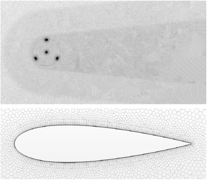
Examples of the mesh used in the STAR-CCM + VAWT simulations showing the wake refinement regions and the turbine blade with prism layers.
To form a wake model based on relevant nondimensional parameters, we used tip-speed ratio (TSR) and solidity to describe aspects of speed and geometry, respectively. We ran CFD simulations at 23 TSRs ranging from 1.5 to 7.0 and five solidities ranging from 0.15 to 1.0 based on the 12 kW H-rotor VAWT from Uppsala University with a 6 meter diameter and three NACA 0021 blades (each with an original 0.25 meter chord length; Kjellin et al., 2011). We also ran four simulations at each TSR/solidity configuration with slightly varying Reynolds numbers in the range of 5 to 6 million resulting in 460 simulations total. Figure 2 shows examples of the time-averaged velocity and vorticity distributions the CFD simulations produced at a TSR of 4.5 and a solidity of 0.25.
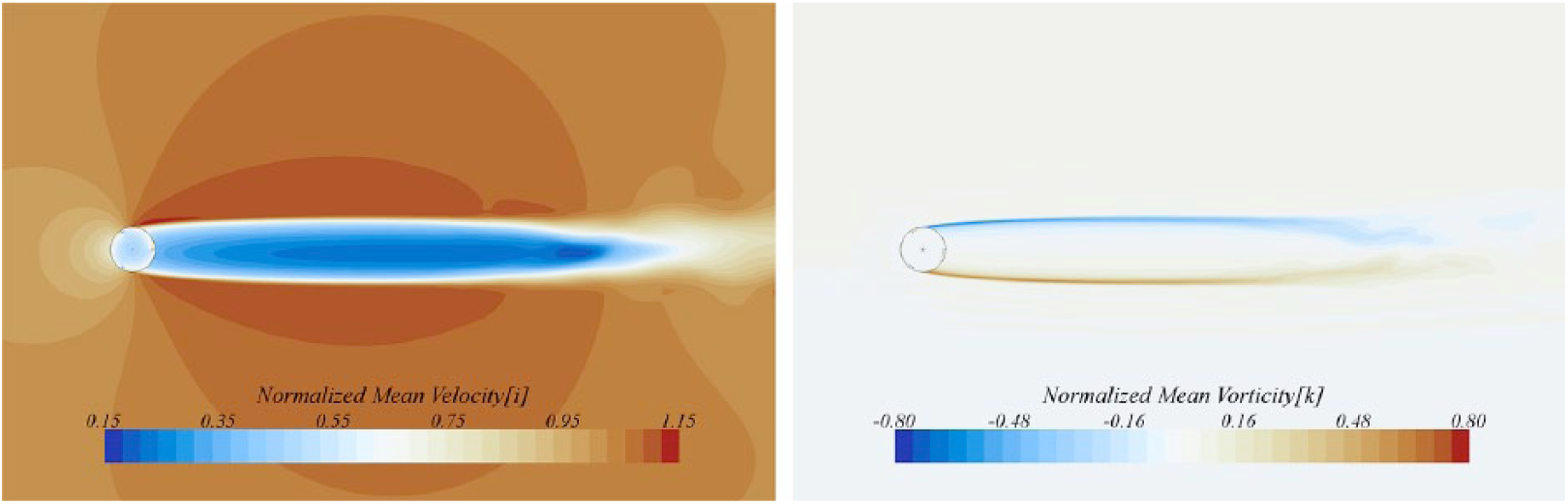
Examples of the time-averaged x-velocity and vorticity distributions of the CFD model at a TSR of 4.5 and a solidity of 0.25. The x-velocity is normalized by the free stream wind velocity of 8.87 m/s and the vorticity by the rotational rate of 13.3 rad/s.
We extracted numerical data from individual cells obtained from 30 lateral cuts of the time-averaged wake, illustrated in Figure 3, to a point downstream where the wake had effectively decayed, ranging from 2 to 35 diameters downstream based on TSR and solidity. We attempted to create a wake model based directly on velocity data. The benefits of a velocity-based model include rapid computation time and easy extendability. However, one of the difficulties in fitting the distribution was its complex shape consisting of induced velocities in both the x- and y-directions all around the turbine (seen in Figure 2). There was also a slight wind velocity increase on the edges of the main deficit region. We implemented combinations of Gaussian, quadratic, exponential, power, and piecewise distributions to attempt fitting the complex data. This resulted in a very complex equation with an extensive data implementation that lacked sufficient accuracy, as shown in Figure 4(a). In contrast, the vorticity stayed within concentrated regions (shown in Figure 2) and was found to be easier to model. We then used the vorticity field to reconstruct the velocity field.
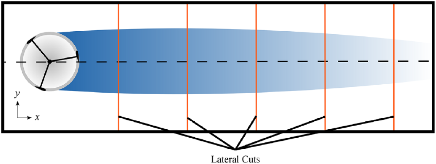
A representation of the lateral cuts made to analyze the wake data numerically. The downstream

An example of the time-averaged x-velocity
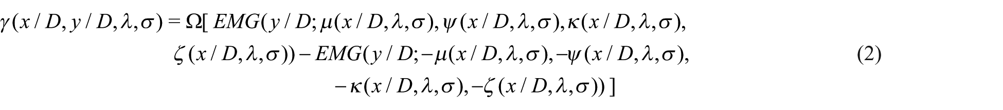
One of the benefits of using a vorticity-based model is that in 2D the vorticity is one-dimensional (z-direction), and through integration it can produce induced velocities in the x- and y-directions in front, to the sides, and behind the turbine. The ability to calculate induced velocities is important to model VAWT pairs placed close together for increased power production as shown in other research efforts (Dabiri, 2011; Ning, 2016; Zanforlin and Nishino, 2016). After exploring several probability distributions to capture the trends in the time-averaged vorticity data, such as the skewed normal, Gompertz, and Weibull distributions, we attained the best fit with the lowest error using the probability density function of an exponentially modified Gaussian (EMG) distribution, defined in equation (1) with respect to the normalized lateral position

Wake model development
An engineering wake model’s purpose is to calculate turbine wake velocity deficits quickly albeit with some compromise in accuracy. In large-scale wind farm analysis and optimization, fast computational times are required to produce velocity calculations at every turbine within a matter of minutes. While the CFD model produced high-fidelity wake data, it was time-consuming to run a single VAWT simulation and would take significantly longer for larger numbers of turbines. Therefore, the improved performance of reduced-order wake models was needed to use the CFD wake data in a wind farm application. In producing our wake model with EMG distributions, we found that the vorticity magnitude and distribution varied in the downstream and lateral directions as well as across TSRs and solidities. Therefore, parameterization of the EMG variables across each of these dimensions created a usable model for a wind farm with continuously varying turbine positions and operating conditions. The vorticity data also varied slightly at different Reynolds numbers. However, the Reynolds number was not used as an input parameter, but rather used to increase the robustness of the EMG distribution fit.
The EMG parameters µ,

A diagram illustrating the relationship between the polynomial surfaces, the EMG parameter distributions (a quadratic distribution for µ in this case), and the vorticity strength
The different combinations of EMG parameter distributions and polynomial surfaces to fit the vorticity data resulted in over 380 billion possibilities. To reduce this to a more manageable set, initial independent surface fits were made of the data across TSR and solidity. The two polynomial surface combinations with the lowest average r-squared errors were chosen, reducing the possibilities to under 14,000. To determine the final polynomial surfaces, we used hold-out cross-validation of all the CFD vorticity data obtained from the 30 lateral cuts at every TSR and solidity configuration and randomly selected 70% of the data to be used as the training set and the remaining 30% as the validation set. This process was done three times and averages of the sum of the squared errors between the fit and the data were computed to reduce any bias that may exist in the training or validation sets. Cross-validation was important in forming our model to eliminate any outliers in the CFD data that may influence behavior specific to that turbine configuration. These outliers could come from unconverged CFD simulations or inconsistent wake behavior.
Using cross-validation with a least-squares regression fitting between the entire CFD vorticity data set and the wake model, we tested distribution combinations and polynomial surface coefficients determined from our initial analysis. As there were multiple results with similar squared errors, we selected the lowest order fit between them, resulting in quadratic (Equation (3)), linear (Equations (4) and (5)), and sigmoid (Equation (6)) distributions as a function of normalized downstream position. The polynomial surfaces required for the resulting 10 distribution coefficients were formed using combinations of second- and third-order fits with respect to TSR and solidity (represented with a subscript number in Equations (3) to (6)). We then retrained the model using all of the CFD vorticity data to produce final polynomial surfaces, such as that shown in Figure 6. With the polynomial surfaces in place to model the EMG parameter coefficients, the model can be easily retrained and tuned to additional wake data sets and various turbulent wind characteristics.


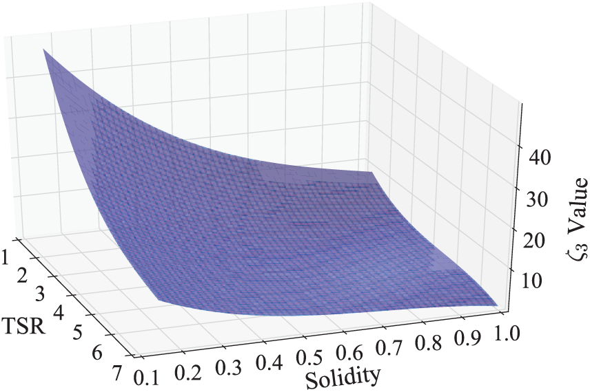
An example of the polynomial surface fit used to calculate
The x- and y-components of the induced wake velocity can be calculated by specifying a downstream
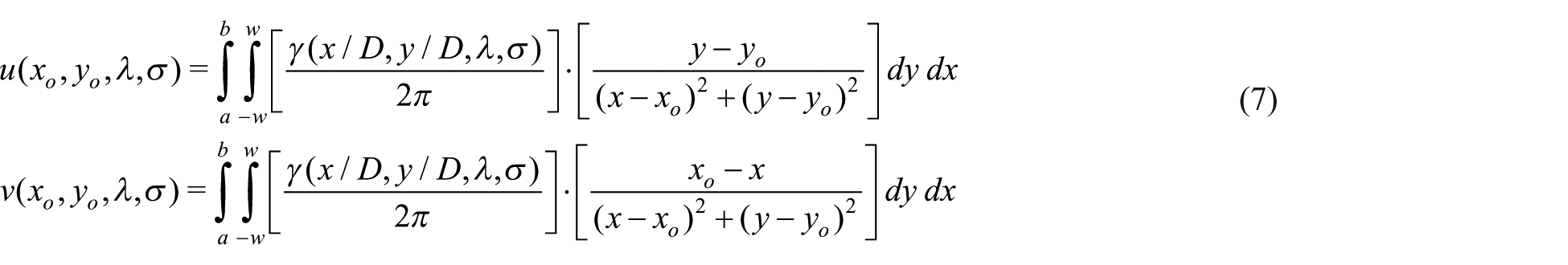
The input parameters define the vorticity strength using equation (2), which is converted to velocity using integration in the downstream direction from the position of the turbine
Wake model results
A reduced-order model increases the speed of wind farm analysis and optimization, but the model’s accuracy in predicting turbine wake velocity deficits must be verified for the model to be of value in real-world situations. The wake velocities calculated by the developed reduced-order VAWT wake model were first compared with the CFD wake velocity data, shown in Figures 7 and 8. The wake model captured the general trends of slower moving wind in front of the turbine, slight wind speed increases on the sides of the wake region, and a decay far enough downstream of the turbine, all with correct velocity magnitudes in the correct regions. While the CFD demonstrated near symmetry with slight asymmetric regions around the wake, the wake model predicted velocities with complete symmetry due to reducing the required EMG parameters by half. In the y-direction, the wake model also predicted the increase in velocity away from the sides of the turbine and the opposite behavior downstream of the turbine.
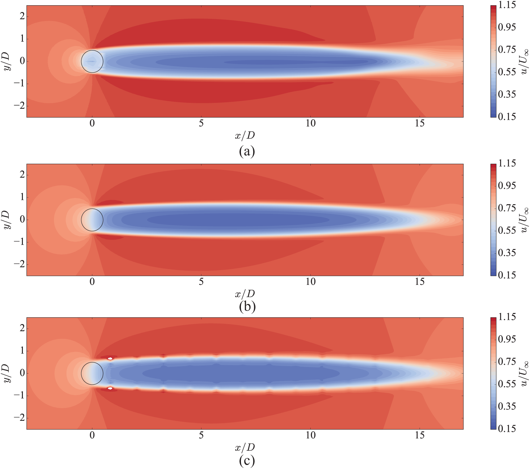
The x-velocity profile calculated by the CFD simulation and the wake model with two integration methods. The downstream
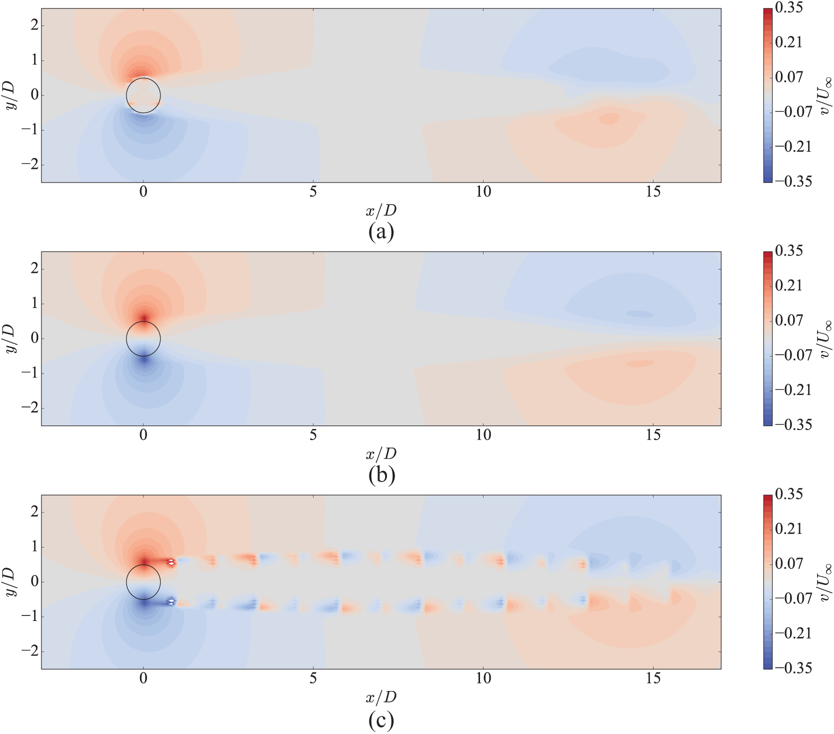
The y-velocity profile calculated by the CFD simulation and the wake model with two integration methods. The downstream
The Simpson’s rule integration created a coarser wake structure (with blips seen on the edge of the wake) due to a smaller number of subdivisions compared with the Gauss–Kronrod method. The coarseness is an acceptable compromise for its speed as a 220 × 200 grid subdivision in the integration (shown in Figures 7(c) and 8(c)) can calculate the velocity at a given point in about 0.02 s with an average percent difference of about 1.1% of the Gauss–Kronrod method, which on average calculates velocity at any point in about 0.3 s. The error of the x-velocity between the two integration methods can be visualized in the error plot of Figure 9 showing the highest errors along the sides of the wake in the coarse regions. As the Simpson’s method would produce less accurate results but would most likely be used for wind farm layout analysis and optimization, the following validation studies are all based on integration using the Simpson’s method understanding that the Gauss–Kronrod method would produce more accurate results with a longer computation time.
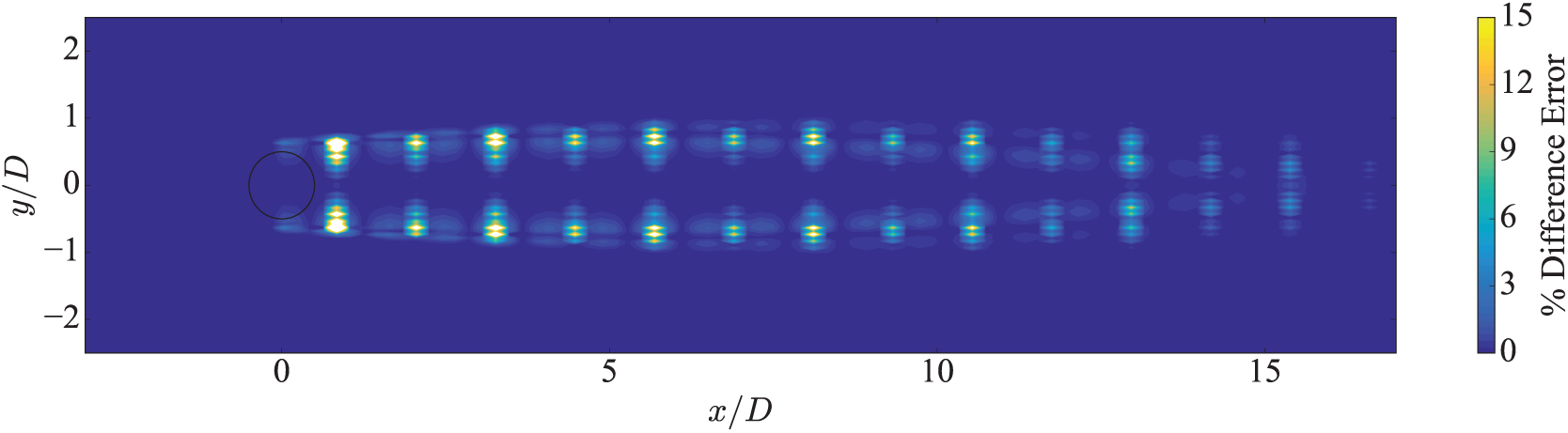
The average percent difference in velocity calculations between the Gauss–Kronrod method and the Simpson’s method based on the velocity calculations shown in Figure 7(b) and (c). The error overall remains near zero with the exception of about 12% of the points along the sides of the wake region where the error exceeds 10% difference. The downstream
The initial wake model was compared with the CFD data at a few locations, which is described in more detail in the previous version of the research (Tingey and Ning, 2016). In this study, we conducted a more comprehensive numerical validation of the updated wake model using a root mean squared (RMS) error normalized by the free stream wind velocity
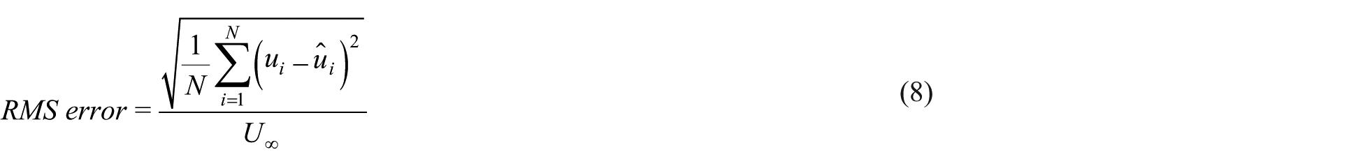
where
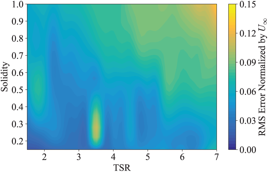
The average normalized RMS error of the velocity deficits predicted by the wake model compared with the CFD data at different TSR and solidity configurations. The values shown are averages of the normalized RMS errors at 2, 4, 6, 8, 10, 15, and 20 diameters downstream.
The wake model was also compared with the experimental PIV study conducted by Tescione et al. (2014) that used a VAWT with two straight NACA 0018 blades and a chord length of 0.06 meters. The turbine had a 1 meter diameter and solidity of 0.24*. The VAWT was tested in 9.3 m/s wind, producing a Reynolds number of about 600,000, and run at a tip-speed ratio of 4.5. The velocity profiles of the PIV, CFD from the validation study of the previous research (Tingey and Ning, 2016), and wake model were compared at six downstream distances as seen in Figure 11. As expected from CFD-based wake data, the wake model follows the near symmetric trend of the CFD data rather than the asymmetry of the experimental data. Overall, the wake model matched the PIV data with an RMS error normalized by the free stream wind velocity of 0.119, slightly higher than the normalized RMS error of 0.113 for the CFD. The percent difference of the maximum velocity deficit of the wake model was 6.3%, also slightly higher than the 5.8% of the CFD.
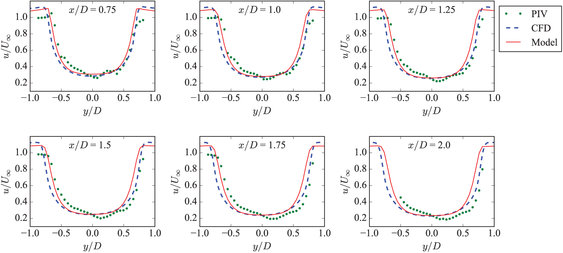
The wake velocity comparison between the PIV study conducted by Tescione et al. (2014), the CFD validation of the previous research (Tingey and Ning, 2016), and our wake model. The x-velocity
For further validation, we also compared our wake model to a wind tunnel study conducted by Battisti et al. (2011). In this study, a three-bladed VAWT with a 1.03 meter diameter was placed in a wind tunnel with a wind speed of about 16 m/s, resulting in a Reynolds number of about 1,000,000. The wind tunnel had a removable test room where the VAWT was placed and tests were run in both a closed configuration (the test room enclosed over the VAWT) and an open configuration (the test room removed and the VAWT open to the outside air). As VAWTs are generally operated in the open, we used the open configuration data to compare with our wake model. The wake velocity was recorded 1.5 diameters downstream of the turbine and the data were overlaid with the wake model’s calculations, which is shown in Figure 12.
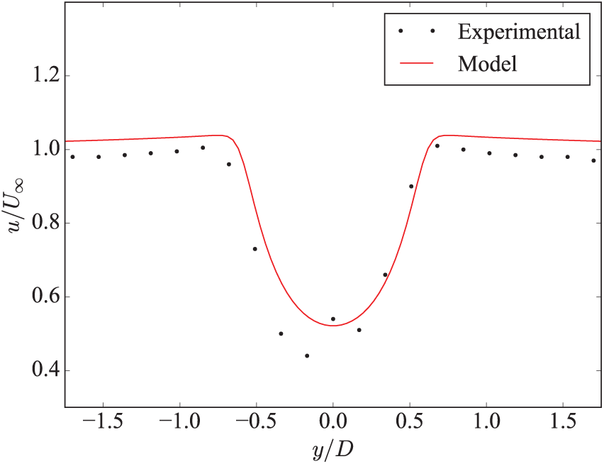
The wake velocity comparison between the wind tunnel study conducted by Battisti et al. (2011) and our wake model at 1.5 diameters downstream. The x-velocity
As seen in Figure 12, the wake model compared with the experimental results had a normalized RMS error of 0.061. The percent difference of the maximum velocity deficit was 14.6%. It is important to note that the two experimental studies were performed with different turbine geometries and setups than the original CFD training set used to create the wake model, which used the specifications of Kjellin et al. (2011). This demonstrates the wake model’s robustness and applicability to different turbine geometric configurations. The model makes some simplifications, like symmetry, but the level of error was deemed to be appropriate for early conceptual design studies, similar to what might be used with a simplified HAWT engineering wake model.
Power calculation
The developed wake model can be used to make rapid velocity predictions for a given TSR and solidity. However, the wake model’s applicability in wind farm layout optimization requires the ability to calculate VAWT power production with multiple wake interactions. To account for overlapping wakes from
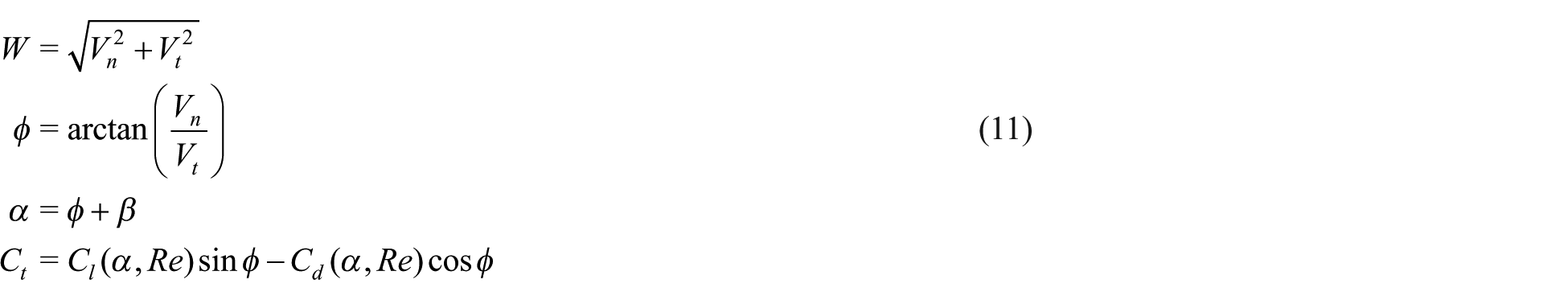
Unlike a HAWT, using the relative center-of-hub velocity to predict the change in power was found to be far too inaccurate. Instead, a more detailed method is necessary based on integration of power contributions around the swept area of the VAWT. Our method is motivated by the actuator cylinder (AC) method developed by Madsen (1982) and extended by Ning (2016). With slight modifications to include the effects of the wake model induced velocities (

with the ± being positive for counter-clockwise rotation and negative for clockwise rotation. New velocity magnitudes
These same equations are used to calculate baseline velocity magnitudes

Using this power calculation method, a pair of counter-rotating Mariah Windspire 1.2 kW VAWTs, each with a diameter of 1.2 meters, were positioned two diameters away from each other at a TSR of 2.625, and the total turbine power normalized by the power of both turbines in isolation from various wind directions was plotted in Figure 13. This same process was done in a CFD study by Zanforlin and Nishino (2016) and the AC study by Ning (2016), each of which are also plotted in Figure 13. From the plot, the three follow the same trends of slight power increases when the turbines are positioned perpendicular to the wind and significant decreases when the turbine wakes impact each other. The biggest difference with the wake model is when the turbines are downstream of each other where there is high uncertainty and the assumptions of baseline velocity components cause irregularities. Additional losses could easily be added in fully waked regions, but in general the optimizer will push turbines out of those locations anyway. This validation study shows the ability of the wake model to predict reasonable power measurements needed for early-stage conceptual wind farm layout optimization studies.

The normalized power of two counter-rotating Mariah Windspire 1.2 kW VAWTs two diameters apart at a TSR of 2.625 as a function of wind direction (the two black dots represent the orientation of the turbines with respect to the wind). Calculated values using the CFD model from Zanforlin and Nishino (2016) and the AC model from Ning (2016) are shown.
Conclusion
As wind farm designs increasingly look to offshore and urban environments, VAWTs may be an effective approach due to their simpler design and operation. With the wake model presented in this article, wake velocities can be evaluated rapidly in the streamwise and crosswind direction and, while various simplifications have been made, the model shows an appropriate level of accuracy of early-stage conceptual design studies. The model was developed by creating a large CFD vorticity database and reducing the data to a fit developed through cross-validation. The model fit is parameterized by TSR and solidity allowing for use across a range of turbines within a TSR between 1.5 and 7.0 and a solidity between 0.15 and 1.0. Reasonable agreement was found against validation studies with Reynolds numbers between about 600,000 and 6,000,000.
As compared with the original CFD data, we found a normalized RMS error of 0.059, with a few configurations reaching as high as 0.230 at specific downstream locations. Some sacrifice in accuracy allowed for a reduction in computation time that was of the order of a day to a model that was of the order of a hundredth of a second. This level of speed is needed for large-scale design optimization studies that combine many turbines and require many iterations. Comparing the wake model with PIV and wind tunnel experiments for completely different turbines, we found that the model matched the experiments with a normalized RMS error of 0.119 in one and 0.061 in the other.
This wake model is intended to be an initial step in parameterizing VAWT wakes in two dimensions, similar to the widely used Jensen (1983) model. The goal was not to produce highly accurate velocity distributions, but rather to produce reasonable power predictions for early-stage wind farm layout optimization. Many opportunities for improvement exist. Studies have shown that influences of finite blades and ground effects influence the propagation of wakes, requiring extensions of the wake model to three-dimensions. Curved-bladed Darrieus VAWTs would also require modifications of the wake model, which assumes straight-bladed VAWTs. The likelihood of blade stall at low TSRs is also better modeled in three-dimensions. Symmetry was assumed in this model, but velocity asymmetries may produce noticeable changes in power for some configurations. Turbulence intensity and, to a lesser degree, stratification are important parameters for wind turbine wakes that should be incorporated into future versions of the model.
Most of these improvements can be added just by supplying new data. The wake model is not meant to be a static, final wake model based only on the CFD vorticity data. Rather, it is intended to be extendable by adding more velocity data (both experimental and simulated). The polynomial surfaces can be retrained with new data to increase the model’s accuracy. The code of our wake model and all of the data sets presented in this article can be openly accessed at the BYU FLOW Lab website. 1
Footnotes
Appendix 1
Acknowledgements
We thank Dr. Fernando Porté-Agel, Dr. Sina Shamsoddin, and Giuseppe Tescione for their assistance in obtaining experimental VAWT wake data sets for our validation studies.
Declaration of conflicting interests
The author(s) declared no potential conflicts of interest with respect to the research, authorship, and/or publication of this article.
Funding
The author(s) received no financial support for the research, authorship, and/or publication of this article.
*
While the solidity reported in the study is 0.11, this current research calculates solidity with respect to the turbine radius instead of diameter. This variation produces a solidity differing by a factor of 2.