Short-term wind power prediction based on improved sparrow search algorithm optimized long short-term memory with peephole connections

Abstract

Accurate short-term wind power prediction is of great significance for the scheduling and management of wind farms. This paper proposes a model for short-term wind power prediction. Firstly, on the basis of traditional long short-term memory network, the peephole connections is added. The improved long short-term memory network is more stable compared to traditional long short-term memory neural networks and is suitable for regression prediction. Secondly, chaotic mapping, adaptive weights, Cauchy mutation, and opposition-based learning strategies are introduced to improve the sparrow search algorithm, and applied to optimize the four hyper-parameters of the long short-term memory network, greatly improving the prediction accuracy of the network. The effectiveness of the model is validated using two short-term wind power datasets with sampling times of 10 and 30 minutes respectively, combined with some fitting curves and performance indicators. The comparison results indicate that the proposed short-term wind power prediction model has high prediction accuracy.

Keywords

Short-term wind power prediction improved sparrow search algorithm long short-term memory peephole connections

Introduction

Background

Wind energy has excellent characteristics such as pollution-free, wide distribution, and large reserves, making it the most promising renewable energy source for large-scale development. Wind power generation, as the main development method of wind energy, has received widespread attention worldwide (Priyadarshi et al., 2024). The technology of wind power generation is becoming increasingly mature, and the degree of scale and commercialization is also gradually increasing. The rapid development of wind power generation has effectively alleviated the difficulties faced by sustainable energy development, resulting in huge economic and social benefits.

The intermittency, volatility, and randomness of wind energy determine that wind power has a large range of fluctuations and a fast rate of change. Therefore, the adverse effects of large-scale wind power grid connection on the power grid are constantly highlighted, posing higher requirements for the planning, scheduling, and operation of the power system. To effectively solve the problem of wind abandonment and improve the dispatch and operation capability of the power system, it is necessary to rely on accurate prediction of wind power output power. The accuracy of wind power prediction directly affects the scheduling optimization results of the power grid (Klaiber and Van Dinther, 2024). At present, the accuracy of wind power prediction is difficult to meet the requirements of scheduling operation, and wind turbines do not have the schedulability of conventional units. The reverse peak shaving characteristics of wind turbines will exacerbate the peak valley difference of system load, increasing the demand for system peak shaving capacity and backup capacity.

According to the time scale of prediction, wind power prediction is usually divided into short-term prediction, medium-term prediction, and long-term prediction. The time scale for short-term prediction is hours, usually predicting the output power in the next few hours 24–48 hours in advance, mainly for the convenience of power grid scheduling to adjust the scheduling plan in a timely manner and ensure power supply quality. Compared to wind power prediction at other time scales, short-term wind power prediction has greater theoretical and practical significance (Li et al., 2023a).

Related works

In recent years, many scholars have conducted research on short-term wind power prediction models. Usually, short-term wind power prediction can be divided into statistical method, intelligent prediction method, physical method, and combination and ensemble prediction method.

Statistical method. The basic idea of a prediction model based on statistical methods is to establish a mapping relationship between the input of the system (numerical weather prediction data, historical measured operating data) and wind power, which is usually a linear relationship that can be explicitly represented by a function. For example, using regression fitting method (Jing and Zhao, 2023), exponential smoothing method (Zheng and Jin, 2022), gray model (Liu et al., 2023a), etc. These models make predictions by capturing effective data and correlation information related to time and space in the data. The prediction accuracy of these method decrease with the increase of the prediction time scale. Statistical methods are generally more sensitive to parameters, have higher prediction accuracy for stationary time series, and have lower prediction accuracy for unstable wind power. The input data of statistical models are usually historical wind speed, wind power output data, and SCADA real-time data from a period prior to the prediction time, and numerical weather prediction data can be used as model input to improve the accuracy of wind power prediction to a certain extent. Due to the simple calculation process and model structure of statistical models, which have good stability in the short-term, they are often used as benchmark models in research to evaluate the predictive performance of other models. The persistence model is the most commonly used benchmark model in statistical models, used to evaluate other prediction models (Sun et al., 2014). It is only considered a valuable prediction method when the prediction accuracy of an advanced method is better than that of the persistence method. The autoregressive model is a widely used model in the early stages of wind power prediction development. In addition, the auto regressive moving average (ARMA) model has also been widely used (Li et al., 2014). Due to ARMA’s strict requirements for the stationarity of time series, wind power time series often cannot meet the stationarity conditions. In order to solve the non-stationary nature of wind power time series, auto regressive integrated moving average (ARIMA) model can be used to establish corresponding prediction models (Li et al., 2022). However, statistical models generally fit the linear relationship between wind power and input data, while in reality, the data is non-linear. Therefore, the accuracy of statistical models for predicting wind power is relatively limited.

Intelligent prediction method. Machine learning related models have also developed rapidly in the field of wind power prediction, such as artificial neural networks (Kari et al., 2023; Wang and Li, 2023), support vector machines (SVM) (Yu et al., 2023), Bayesian networks (Liu et al., 2023b), deep learning models (Niksa-Rynkiewicz et al., 2023; Wei et al., 2023; Xu et al., 2023), etc. Other methods such as Fuzzy logic models (Khasanzoda et al., 2022) and Kalman filter (Ishikawa et al., 2017) have also been applied in the prediction of wind power. The essence of intelligent methods is to establish the relationship between input vectors and output variables through learning and training a large amount of historical operational measured data. It is a black box model, rather than explicitly describing it in the form of analytical methods. The model built by this method is usually a nonlinear model, which can more accurately fit the nonlinear relationship and non-stationary nature between wind power and wind speed, as well as the wind power time series itself, reflecting the fluctuation characteristics of wind power, the prediction accuracy is high. Intelligent prediction models also have some shortcomings. Artificial neural networks require a large amount of historical data and tedious parameter adjustment processes. The accuracy of support vector machines is greatly influenced by parameters, resulting in complex training processes and long training times. Deep learning models require a large number of samples and high time complexity costs, which must also be considered. Fuzzy logic models have higher complexity and require longer processing time when there are many rules. Bayesian networks require the professional level and experience of modelers. The Kalman filter model requires information from the previous system.

Physical method. The essence of a physical model is to improve the resolution of a numerical weather prediction model (Zeng et al., 2023), enabling it to accurately predict weather parameters such as wind speed, direction, pressure, and temperature at a certain point (such as at each wind turbine). Based on the weather forecast variables such as wind speed, direction, pressure, and temperature predicted by the numerical weather prediction model, as well as geographic and terrain factors and contour lines around the wind farm, using micro meteorology theory and computational fluid dynamics methods, calculate meteorological information such as wind speed and direction at the height of the wind turbine hub, and then calculate the power prediction results for each wind turbine based on the power curve of the wind turbine. Due to the low update frequency of numerical weather prediction data, physical methods are more suitable for medium to long-term wind power prediction, but not for short-term wind power prediction (Saini et al., 2023). Meanwhile, many wind farms are unable to obtain meteorological data.

Combination and ensemble prediction method. A single prediction model for wind power prediction may have good prediction performance in specific prediction environments, but it can also lead to significant errors at certain measurement points and may not achieve high accuracy prediction results in all cases. Therefore, in order to optimize the prediction process and improve prediction accuracy, using a combination of multiple models has gradually become a popular research approach. Combination prediction methods can establish combination prediction models based on the technical characteristics and advantages of each model, overcome the limitations of individual prediction models, and effectively reduce the probability of large error points. According to the definition and modeling differences of combination prediction methods, they can be divided into four categories. The first method is a combination prediction method based on weight coefficients (Duan et al., 2022; Liu et al., 2022). The weighting process of wind power combination prediction is to allocate appropriate weight coefficients based on the relative effectiveness of each individual model, reflecting the importance of the model in the combination model. The second method is a combination prediction method based on data preprocessing. The data preprocessing model can decompose nonlinear wind power or wind speed time series into stable subsequences that are easy to analyze and predict. In addition, it can filter out irrelevant or residual feature quantities in the data, improve the quality of the original data, and avoid redundant calculation processes. Common decomposition algorithms include wavelet transform (Zhang et al., 2023), ensemble empirical model decomposition (Du et al., 2023), variational model decomposition (Qin et al., 2023), etc. The third method is a combination prediction method based on model parameter optimization. Parameter selection and optimization methods can play a certain role in improving the prediction performance during the model training process. Swarm algorithms are the most common optimization algorithms in wind power prediction. Some newest algorithms include whale optimization algorithm (Saeed et al., 2023), wolf optimization algorithm (Cai et al., 2023), sparrow optimization algorithm (Awadallah et al., 2023), etc.

Main work

This paper mainly discusses the prediction of short-term wind power. A prediction approach combining swarm intelligence optimization algorithm and deep learning model is adopted, with short-term wind power as the research object. The performance of the model is verified through actual collected wind farm data. In summary, the main innovations of this paper are as follows.

Choose an improved long short-term memory (LSTM) with peephole connections as the short-term wind power prediction model. Each gate in the improved LSTM can peek at the unit state, improving prediction accuracy.

On the basis of the standard sparrow search algorithm (SSA), an improved SSA (ISSA) is proposed by combining Cauchy mutation optimization and opposition-based learning. Compared with the standard SSA, it reduces the possibility of falling into local optimal, improves the convergence accuracy and development ability of the algorithm.

The ISSA is used to optimize the hyper-parameters of the improved LSTM model, greatly enhancing the predictive ability of the improved LSTM.

Structure of the paper

Other contents of this study are as follows. Section 2 introduces the basic theory of LSTM with peephole connections. Section 3 gives the introduction to the process of ISSA and tested its benchmark function. In Section 4, the implementation process of ISSA optimized improved LSTM for short-term wind power prediction is described. Section 5 verifies the effectiveness of the proposed short-term wind power prediction model. The last section gives the conclusion and future work.

LSTM with peephole connections

LSTM is essentially a type of recurrent neural network (RNN). However, RNN is unable to effectively utilize earlier historical information, resulting in long-term dependencies issues. LSTM addressed the shortcomings of RNN, as it can learn long-term dependencies (Li et al., 2024a). The LSTM has been designed to solve the problem of long-term dependencies, and the solution is that the LSTM network can remember longer historical information. Unlike RNN networks, LSTM has a different repetitive module structure. Neural networks typically have one layer, but LSTM has four layers and uses special processing methods for interaction.

Compared to RNN, LSTM can learn the target more effectively in cases of long time lag. However, if precise calculation of time is required in a long lag, LSTM cannot achieve it. This paper introduces an improved LSTM, which adds peephole connections to the traditional LSTM network model. The improved LSTM network is more stable compared to traditional LSTM networks and is more suitable for regression prediction problems such as short-term wind power. The structure of the improved LSTM network is shown in Figure 1. The implementation process of the forgetting gate is shown in equation (1). The implementation process of the input gate is shown in equations (2)∼(4). The structure of the output gate is shown in equations (5) & (6).

f_{t} = σ (W_{f} \cdot [C_{t - 1}, h_{t - 1}, x_{t}] + b_{f})

(1)

i_{t} = σ (W_{i} \cdot [C_{t - 1}, h_{t - 1}, x_{t}] + b_{i})

(2)

{\bar{C}}_{t} = \tanh (W_{C} \cdot [h_{t - 1}, x_{t}] + b_{C})

(3)

C_{t} = f_{t} * C_{t - 1} + i_{t} * {\bar{C}}_{t}

(4)

o_{t} = σ (W_{o} \cdot [C_{t}, h_{t - 1}, x_{t}] + b_{o})

(5)

h_{t} = o_{t} * \tanh (C_{t})

(6)

where $h_{t - 1}$ is the previous output in any LSTM unit, $x_{t}$ is the current input in any unit of LSTM, $C_{t - 1}$ is the previous input status value, $f_{t}$ is the forgetting gate, tanh is the basic structure layer of the tan layer in LSTM, $i_{t}$ and ${\bar{C}}_{t}$ are the variables in the input gate, $h_{t}$ is the current output in any unit, $o_{t}$ is the variable in the output gate.

Figure 1.

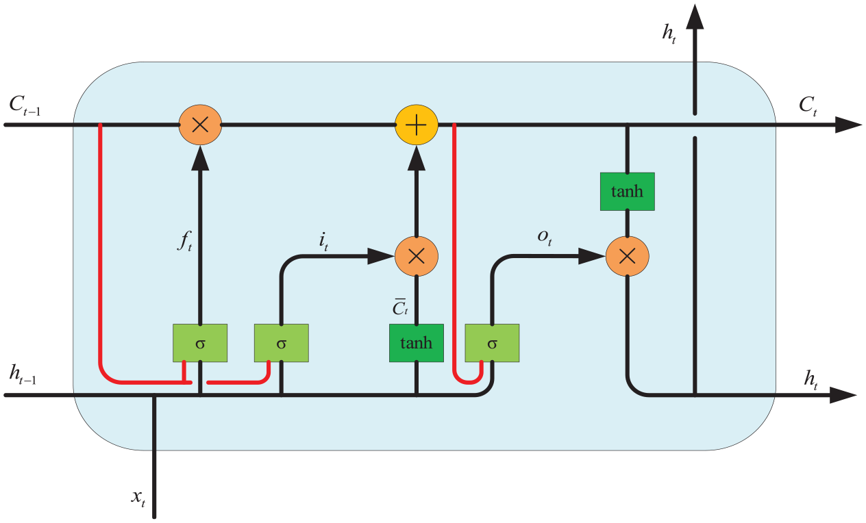
The structure of the LSTM with peephole connections.

The LSTM network contains one or more memory cells. It also includes three adaptive memory blocks with added gating units, which are shared by all cells in the block. The core of each memory cell has a cyclic self connecting linear unit called constant error carousel (CEC). CEC allows LSTM to be applied across large time lags (1000 discrete time steps or more) between objects, and this algorithm can directly obtain cell outputs. But if the output gate is disabled, the output will approach 0, and the lack of information may damage the performance of the network. Therefore, by adding peephole connections from CEC to the same memory block, LSTM cells can be expanded to examine their current internal state. Even if the target signal lacks information, the LSTM model can perform precise and stable learning without a mentor.

When LSTM networks are applied to regression prediction, many parameters affect the final performance. The most important parameters include number of neurons in the first layer LSTM unit (L1), number of neurons in the second layer LSTM unit (L2), learning rate (LR), and iterations (ITR). The three parameters L1, L2, and LR affect the performance of the LSTM network, while LR affects the speed of the LSTM network. This paper uses an ISSA to optimize the hyper-parameters of the LSTM network.

ISSA

In this section, improvements are made to SSA to achieve ISSA, and its performance is tested.

Implementation of ISSA

SSA is first proposed in 2020 as a new swarm intelligence optimization algorithm (Xue and Shen, 2020). Compared with other optimization algorithms such as particle swarm optimization or differential evolution, SSA has the advantages of fast iteration speed, fast convergence speed, accurate extreme value optimization, and high solving efficiency (Geng et al., 2023; Yue et al., 2023). On the other hand, SSA has shown superior capabilities in function optimization problems compared to swarm intelligence algorithms such as particle swarm optimization and gray wolf optimization. It also has the characteristics of easy implementation and adjustment, making it suitable for solving complex optimization problems with low dependence on initial solutions and adapting to different types of problems, such as capacity configuration of wind-solar-diesel-storage (Dong et al., 2022), path planning for mobile robots (Hou et al., 2024; Wei et al., 2024), node localization in wireless sensor networks (Zhang et al., 2022), and so forth. Therefore, this paper chooses SSA and improves it to apply to the parameter optimization of LSTM. The principle of SSA is as follows.

The set matrix is shown in equation (7).

X = {[x_{1}, x_{2}, \cdot \cdot \cdot, x_{K}]}^{T}, x_{k} = [x_{a, 1}, x_{a, 2}, \cdot \cdot \cdot, x_{a, d}]

(7)

where K is the number of sparrows, $a = 1, 2, \cdot \cdot \cdot, K$ , d is the dimension of the variable. The fitness value matrix of sparrows is shown in equations (8)∼(9).

F_{x} = {[f (x_{1}), f (x_{2}), \cdot \cdot \cdot, f (x_{K})]}^{T}

(8)

f (x_{a}) = [f (x_{a, 1}), f (x_{a, 2}), \cdot \cdot \cdot, f (x_{a, d})]

(9)

where $F_{x}$ represents the individual’s fitness value. The location update method of the discoverer is shown in equation (10).

X_{a, b}^{t + 1} = {\begin{matrix} X_{a, b}^{t} \cdot \exp (\frac{- a}{α \cdot i t_{max}}) R < S \\ X_{a, b}^{t} + D_{Gaussian} \cdot L R \geq S \end{matrix}

(10)

where $X_{a, b}^{t}$ is the position of the a-th sparrow in the b-th dimension, t represents the current number of iterations, $b = 1, 2, \cdot \cdot \cdot, d$ , $i t_{max}$ is the maximum number of iterations, $α \in (0, 1)$ and $α$ is a random number, R is the warning value and $R \in [0, 1]$ , S is the safety value and $S \in [0.5, 1]$ , $D_{Gaussian}$ is a random number that follows a normal distribution of [0,1], $L$ is a $1 \times d$ dimensional matrix. The formula for updating the follower’s position is shown in equation (11).

X_{a, b}^{t + 1} = {\begin{matrix} D_{Gaussian} \cdot \exp (\frac{X_{worst}^{t} - X_{a, b}^{t}}{a^{2}}) a > \frac{N}{2} \\ X_{p}^{t + 1} + | X_{a, b}^{t} - X_{p}^{t + 1} | \cdot A^{T} {(A A^{T})}^{- 1} \cdot L other \end{matrix}

(11)

where $X_{worst}^{t}$ is the worst global position, A is a $1 \times d$ dimensional matrix, and each element in A is randomly assigned a value of 1 or −1. The investigation warning method is shown in equation (12).

X_{a, b}^{t + 1} = {\begin{matrix} X_{best}^{t} + β | X_{a, b}^{t} - X_{best}^{t} | f_{a} > f_{c} \\ X_{a, b}^{t} + k^{*} \cdot \frac{| X_{a, b}^{t} - X_{worst}^{t} |}{f_{a} - f_{d} + ε} f_{a} = f_{c} \end{matrix}

(12)

where, $X_{best}$ represents the global best position; $β$ is the step size adjustment coefficient, which is a normally distributed random number with a mean of 0 and a variance of 1; $k^{*} \in [- 1, 1]$ , and is a uniform random number; $f_{a}$ is the current fitness value of sparrows; $f_{c}$ is the current global optimal fitness value; $ε$ is the minimum constant to avoid a denominator of 0.

Standard SSA has local extremum problems. Therefore, this paper proposes ISSA, which principles are as follows.

Sin chaotic initialization population

The population initialization of the sparrow algorithm is carried out using Sin chaotic, and the expression of the one-dimensional self-mapping of Sin chaotic is shown in equation (13).

{\begin{matrix} x_{k + 1} = \sin (2 / x_{k}) k = 0, 1, \cdot \cdot \cdot, K \\ - 1 \leq x_{k} \leq 1 x_{k} \neq 0 \end{matrix}

(13)

Dynamic adaptive weight factor

In the initial stage of SSA, the discoverer keeps approaching the optimal solution, which limits the search range of the algorithm and leads to falling into local extremes. This paper introduces a dynamic weight factor, which has a larger value in the early stages of iteration and better global search ability. In the later stage of iteration, its value adaptively decreases, which is more conducive to local search. Meanwhile, the convergence speed has significantly improved. The expression for the weight factor is shown in equation (14). The updated location of the improved discoverer is shown in equation (15).

ω = \frac{e^{2 (1 - t / i t_{max})} - e^{- 2 (1 - t / i t_{max})}}{e^{2 (1 - t / i t_{max})} + e^{- 2 (1 - t / i t_{max})}}

(14)

X_{a, b}^{t + 1} = {\begin{matrix} X_{a, b}^{t} + ω (f_{b, c}^{t} - X_{a, b}^{t}) \cdot rand R < S \\ X_{a, b}^{t} + D_{Gaussian} R \geq S \end{matrix}

(15)

where $f_{b, c}^{t}$ is the global optimal solution for the b-th dimension in the previous generation.

Improved update method for warning sparrows

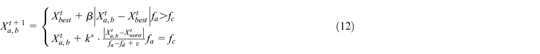
The improved warning sparrow update method is shown in equation (16). According to equation (16), it can be seen that the improved update method expresses that if a sparrow is in the optimal position, it will move to a random position between the optimal and worst positions, or to a random position between itself and the optimal position, thereby increasing the diversity of optimization solutions.

X_{a, b}^{t + 1} = {\begin{matrix} X_{best}^{t} + β (X_{a, b}^{t} - X_{best}^{t}) f_{a} \neq f_{c} \\ X_{best}^{t} + β (X_{worst}^{t} - X_{best}^{t}) f_{a} = f_{c} \end{matrix}

(16)

The fusion of Cauchy mutation and opposition-based learning strategy

In order to help sparrows find the optimal solution, opposition-based learning strategy is integrated into the SSA. Its expression is shown in equations (17)∼(18).

X_{best}^{'} (t) = ub + U \times (lb - X_{best} (t))

(17)

X_{a, b}^{t + 1} = X_{best}^{'} (t) + B \times (X_{best} (t) - X_{best}^{'} (t))

(18)

where, $X_{best}^{'} (t)$ is the inverse solution of the t-th optimal solution, $ub$ represents the upper bound, $lb$ represents the lower bound, $U$ is a random number matrix of $1 \times d$ that follows the [0, 1] standard uniform distribution, B is the control parameter for information exchange.

Introduce Cauchy variation into the equation of the target location. The Cauchy operator has better perturbation ability and improves the global optimization performance of the algorithm. The Cauchy mutation expression is shown in equation (19).

X_{a, b}^{t + 1} = X_{best} (t) + C (0, 1) \times X_{best} (t)

(19)

where $C (0, 1)$ is the standard Cauchy distribution. The generating function is as follows.

η = \tan [(ξ - 0.5) π]

(20)

In order to further improve the optimization performance, this paper adopts a dynamic selection strategy to update the target position, which integrates reverse learning strategy and Cauchy mutation to transform with a certain probability and dynamically update the target position. The calculation formula for selecting probability $P_{s}$ is as follows.

P_{s} = - \exp {(1 - \frac{t}{i t_{max}})}^{20} + θ

(21)

where $θ$ is the adjustment parameter, which is set to 0.05 in this paper. If $rand < P_{s}$ , choose the opposition-based learning strategy, otherwise choose the Cauchy mutation perturbation strategy.

Finally, the greedy rule is introduced to compare the fitness values of two new and old positions and determine whether to update the positions. The greedy rule is shown in equation (22).

{\begin{cases} X_{b e s t} = X_{a, b}^{t + 1} f (X_{a, b}^{t + 1}) < f (X_{b e s t}) \\ X_{b e s t} = X_{b e s t} f (X_{a, b}^{t + 1}) \geq f (X_{b e s t}) \end{cases}

(22)

The specific implementation steps of the proposed ISSA are as follows.

Step 1 Parameter initialization. Including population size $N$ , maximum number of iterations $i t_{max}$ , proportion of discoverers $PD$ , proportion of warning $SD$ , warning threshold R, etc. According to equation (13), initialize the sparrow population.

Step 2 Calculate the fitness of sparrows, identify the optimal and worst values of fitness, as well as their corresponding positions.

Step 3 Select some sparrows from the better ones as discoverers and update their positions according to equation (15).

Step 4 The remaining sparrows, as followers, update their positions according to equation (11).

Step 5 Randomly select a portion of sparrows as warning sparrows and update their positions according to equation (16).

Step 6 Using Cauchy mutation perturbation strategy and opposition-based strategy to perturb the current optimal solution and obtain a new optimal solution.

Step 7 According to the greedy rule (22), decide whether to update the position.

Step 8 Determine if the end condition is met. If yes, proceed to the next step; otherwise, return to Step 2.

Step 9 End the algorithm and output the optimal results.

Performance analysis of ISSA

To verify the optimization performance of ISSA, the optimization design problem of pressure vessels is selected as a test case. The optimization design problem of pressure vessels is a well-known benchmark problem in engineering applications, which can be used to verify the optimization performance of the proposed ISSA. 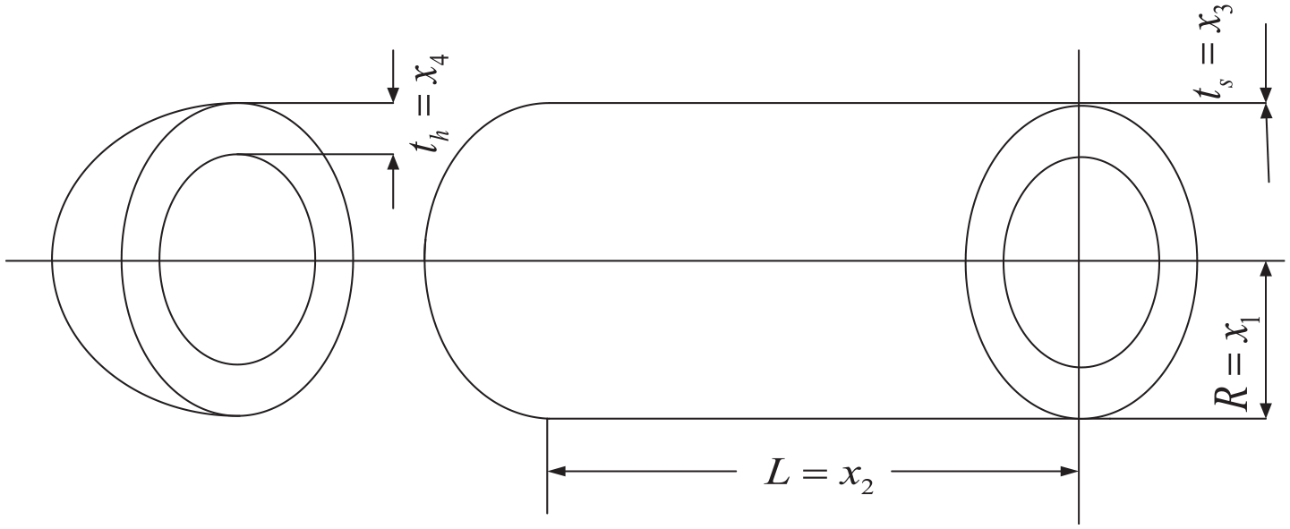As shown in Figure 2, the optimization problem can be described as calculating the optimization design variables $x_{1} (R)$ , $x_{2} (L)$ , $x_{3} (t_{s})$ , and $x_{4} (t_{h})$ to allow the container to accommodate more materials. Among them, $x_{1} (R)$ is the radius of the container; $x_{2} (L)$ is the length of the catheter; $x_{3} (t_{s})$ is the cylinder wall thickness; $x_{4} (t_{h})$ is the thickness of the hemispherical head wall.

Figure 2.

The optimization design problem of pressure vessels.

The process of container optimization design is as follows, with a search variable of $X (x_{1}, x_{2}, x_{3}, x_{4})$ to minimize $f (X)$ . The expression for the problem to be optimized is shown in equation (23).

f (X) = 0.6224 x_{1} x_{2} x_{3} + 1.7781 x_{1}^{2} x_{4} + 3.1661 x_{2} x_{3}^{2} + 19.84 x_{1} x_{3}^{2}

(23)

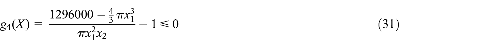
The constraints are as follows.

10 \leq x_{1} \leq 200

(24)

10 \leq x_{2} \leq 200

(25)

0.0625 \leq x_{3} \leq 6.1875

(26)

0.0625 \leq x_{4} \leq 6.1875

(27)

g_{1} (X) = \frac{0.0193 x_{1}}{x_{3}} - 1 \leq 0

(28)

g_{2} (X) = \frac{0.00954 x_{1}}{x_{4}} - 1 \leq 0

(29)

g_{3} (X) = \frac{x_{2}}{240} - 1 \leq 0

(30)

g_{4} (X) = \frac{1296000 - \frac{4}{3} π x_{1}^{3}}{π x_{1}^{2} x_{2}} - 1 \leq 0

(31)

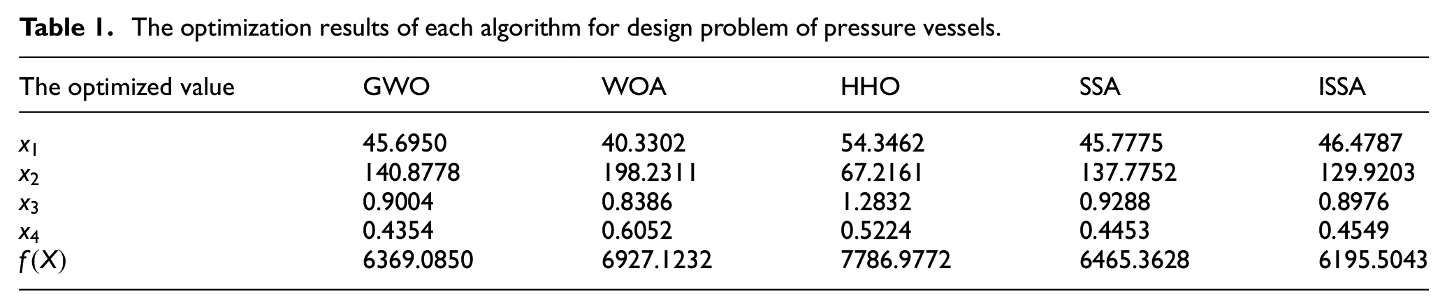
ISSA and SSA are used to optimize the design of pressure vessels separately. Set the iteration times of the two algorithms to 1000 times, the population size is 50, and optimize the average fitness curve after 10 times as shown in Figure 3. From Figure 3, it can be seen that the ISSA has faster convergence speed and better adaptability than the SSA. The results indicate that the ISSA proposed in this paper is effective. After optimization, the optimal solution obtained by the SSA is 45.7775, 137.7752, 0.9288, and 0.4453, and the optimal value of the objective function obtained is 6465.3628. The optimal solution obtained by ISSA is 46.4787, 129.9203, 0.8976, 0.4549, and the optimal value of the objective function obtained by ISSA algorithm is 6195.5043. From the optimization results, the proposed ISSA is more capable of finding the global optimal solution than SSA. Prove that ISSA has improved performance compared to the original SSA, therefore, the optimization of LSTM model by ISSA is feasible.

Figure 3.

Fitness performance comparison between ISSA and SSA.

To further demonstrate the effectiveness of ISSA, gray wolf optimization (GWO) algorithm, whale optimization algorithm (WOA), and Harris Hawks Optimizer (HHO) are selected for comparison. The algorithms are also run 10 times, and the average value is taken as the final result. The maximum number of iterations is 1000, and the population size is 50. In GWO, a is 2 (linearly decreased over iterations). In WOA, a is 2 (linearly decreased over iterations). In HHO, β is 1.5. The optimization results are shown in Table 1. From the results in Table 1, it can be seen that ISSA performs better than SSA and other optimization algorithms, making it very suitable for hyper-parameters optimization in LSTM.

Table 1.

The optimization results of each algorithm for design problem of pressure vessels.

The optimized value	GWO	WOA	HHO	SSA	ISSA
$x_{1}$	45.6950	40.3302	54.3462	45.7775	46.4787
$x_{2}$	140.8778	198.2311	67.2161	137.7752	129.9203
$x_{3}$	0.9004	0.8386	1.2832	0.9288	0.8976
$x_{4}$	0.4354	0.6052	0.5224	0.4453	0.4549
$f (X)$	6369.0850	6927.1232	7786.9772	6465.3628	6195.5043

Designed prediction model

Based on the introduction of the above basic knowledge, the flow chart of the proposed wind power prediction model is shown in Figure 4.

Figure 4.

The flow chart of the proposed wind power prediction model.

According to Figure 4, the specific implementation process of the designed short-term wind power prediction model is as follows.

Step 1 Firstly, collect wind power data and divide it into training and testing sets. In order to eliminate the dimension difference, the data are normalized. Initialize the hyper-parameters of LSTM and ISSA.

Step 2 Input short-term wind power training set data into the LSTM network. Obtain the network output of LSTM.

Step 3 Substitute the four parameters (L1, L2, LR, and ITR) to be optimized for LSTM into ISSA and optimize them according to the introduction in Section 3.1.

Step 4 Calculate the fitness value obtained for the current iteration. Update the optimal sparrow individual within the population based on fitness values. This paper uses the fitness function shown in equation (32) below. Equation (32) represents the root mean square error (RMSE) between the output value of the LSTM network and the actual value. In (32), N is the number of samples, $y_{i}$ is the actual of short-term wind power, ${\bar{y}}_{i}$ is the predicted value by the LSTM network, k is the current number of iterations.

\begin{matrix} fitness (k) = \sqrt{\frac{1}{N} \sum_{i = 1}^{N} (y_{i} - {\bar{y}}_{i})} \\ s . t . {\begin{matrix} L 1 \in [L 1_{min}, L 1_{max}] \\ L 2 \in [L 2_{min}, L 2_{max}] \\ LR \in [L R_{min}, L R_{max}] \\ ITR \in [IT R_{min}, IT R_{max}] \end{matrix} \end{matrix}

(32)

Step 5 Determine whether the termination conditions are met. If it meets the requirements, jump to Step 6. If not satisfied, output the current optimal solution to obtain the four current optimization results (L1, L2, LR, and ITR), and go to Step 2.

Step 6 Optimization completed. Obtain the optimal solutions for L1, L2, LR, and ITR. Establish the corresponding improved LSTM network based on the optimal solutions, and input the test set to obtain the corresponding prediction results. Verify the effectiveness of the model.

Simulation and verification

The effectiveness of the prediction model is verified through actual wind power data. Compared with other prediction models, the comparison results fully demonstrate the effectiveness of this prediction model.

Dataset

This paper collected two sets of short-term wind power datasets from Xintianbao Wind Farm in Tieling City, Liaoning Province, China. The sampling period of the first dataset is 10 minutes, from Unit 2 of the wind farm, named as dataset 1. The sampling period of the second dataset is 30 minutes, from Unit 8 of the wind farm, named as dataset 2. The length of both datasets is 1000. Use the first 800 sets of data as the training set and the last 200 sets of data as the test set. The two collected wind power datasets are shown in Figure 5. From the curve changes in the graph, it can be seen that short-term wind power exhibits non periodic, random, and nonlinear characteristics, making it suitable for verifying the performance of the prediction model.

Figure 5.

The two collected wind power datasets.

Performance indicators

The performance of predictive models can be judged by some performance indicators. This study introduces the following eight widely used performance indicators to evaluate the effectiveness of the model (Li et al., 2024b).

RMSE

RMSE = \sqrt{\frac{1}{N} \sum_{i = 1}^{N} {(w (i) - \bar{w} (i))}^{2}}

(33)

Mean absolute error (MAE)

MAE = \frac{1}{N} \sum_{i = 1}^{N} | w (i) - \bar{w} (i) |

(34)

Mean absolute percentile error (MAPE)

MAPE = \frac{1}{N} \sum_{i = 1}^{N} | w (i) - \bar{w} (i) | \times 100 / w (i)

(35)

Relative root mean square error (RRMSE)

RRMSE = \sqrt{\frac{1}{N} \sum_{i = 1}^{N} {(\frac{w (i) - \bar{w} (i)}{w (i)})}^{2}}

(36)

Square sum error (SSE)

SSE = \sum_{i = 1}^{N} {(w (i) - \bar{w} (i))}^{2}

(37)

$R^{2}$ (R Square)

R^{2} = 1 - \frac{\sum_{i = 1}^{N} {(w (i) - \bar{w} (i))}^{2}}{\sum_{i = 1}^{N} {(w (i) - w_{m})}^{2}}

(38)

Theil inequality coefficient (TIC)

TIC = \frac{\sqrt{\frac{1}{N} {(w (i) - \bar{w} (i))}^{2}}}{\sqrt{\frac{1}{N} \sum_{i = 1}^{N} w {(i)}^{2}} + \sqrt{\frac{1}{N} \sum_{i = 1}^{N} \bar{w} {(i)}^{2}}}

(39)

The index of agreement (IA)

IA = 1 - \frac{\sum_{i = 1}^{N} {(w (i) - \bar{w} (i))}^{2}}{\sum_{i = 1}^{N} {(| \bar{w} (i) - w_{m} | + | w (i) + w_{m} |)}^{2}}

(40)

where, $N$ is number of sample, $w (i)$ is actual value of wind power, $\bar{w} (i)$ is prediction value of wind power, $w_{m}$ is the mean value of wind power.

On the other hand, this paper uses the Diebold-Mariano (DM) test to verify the accuracy of the prediction model under certain confidence levels (Sun et al., 2023). The premise of hypothesis testing is,

H_{0} : E (d_{h}) = 0, \forall n

(41)

H_{1} : E (d_{h}) \neq 0, \exists n

(42)

The statistical value of DM testing is equal to the following equation.

DM = \frac{\sum_{h = 1}^{k} (L (ε_{t + h}^{(A)}) - L (ε_{t + h}^{(B)})) / k}{\sqrt{S^{2} / k}} s^{2}

(43)

where $ε_{t + h}$ is the prediction error, $S^{2}$ is an estimation value for the variance of $d_{h} = L (ε_{t + h}^{(A)}) - L (ε_{t + h}^{(B)})$ , and L is the loss function, which is performed to measure the prediction accuracy. Generally, L can be expressed as deviation error loss or squared error loss. The test statistic of DM testing converges to the standard normal distribution. Given the prediction error of two prediction models and the significance level $α$ , if E (A, B) is greater than 0, it indicates that the predictive performance of model A is inferior to that of model B. If E (A, B) is equal to 0, it indicates that the predictive performance of model A is consistent with that of model B. If E (A, B) is less than 0, it indicates that model A has better predictive performance than model B.

Results

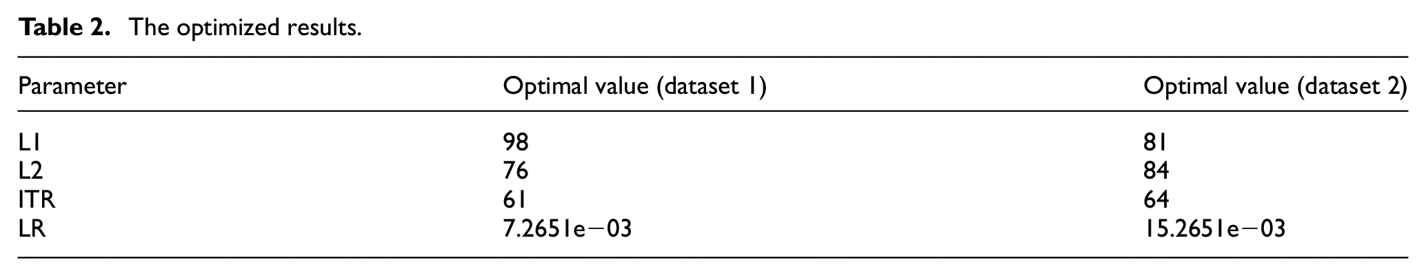
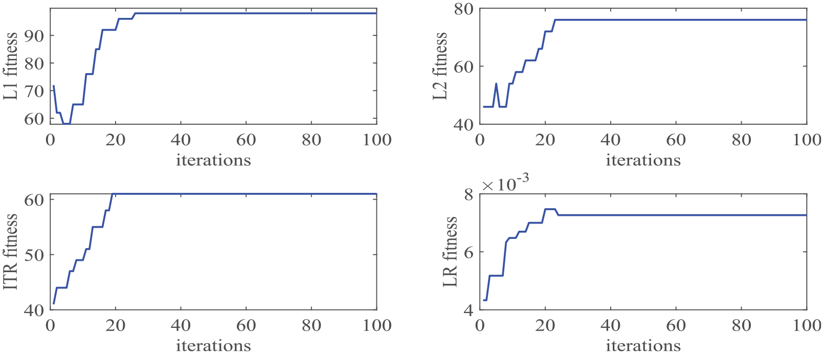
Following the implementation steps of the prediction model introduced above, the LSTM with peephole connections network needs to be optimized first. The four parameters to be optimized and their set upper and lower bounds are $L 1 \in [1, 100]$ , $L 2 \in [1, 100]$ , $LR \in [0.001, 0.1]$ , and $ITR \in [1, 100]$ . The parameters of ISSA are as follows: the population size is 20, maximum number of iterations is 100, warning value (R) is 0.6, proportion of discoverers (PD) is 0.7, proportion of warning (SD) is 0.2. To avoid the randomness caused by optimization algorithms, ISSA runs 20 times and takes the average of each iteration and the final optimization result as the final optimization result. The curves of the four hyper-parameters of the ISSA optimized LSTM network for two datasets is shown in Figures 6 and 7. The obtained optimal parameters of the LSTM are shown in Table 2.

Figure 6.

Fitness of hyper-parameters in LSTM network based on ISSA (dataset 1).

Figure 7.

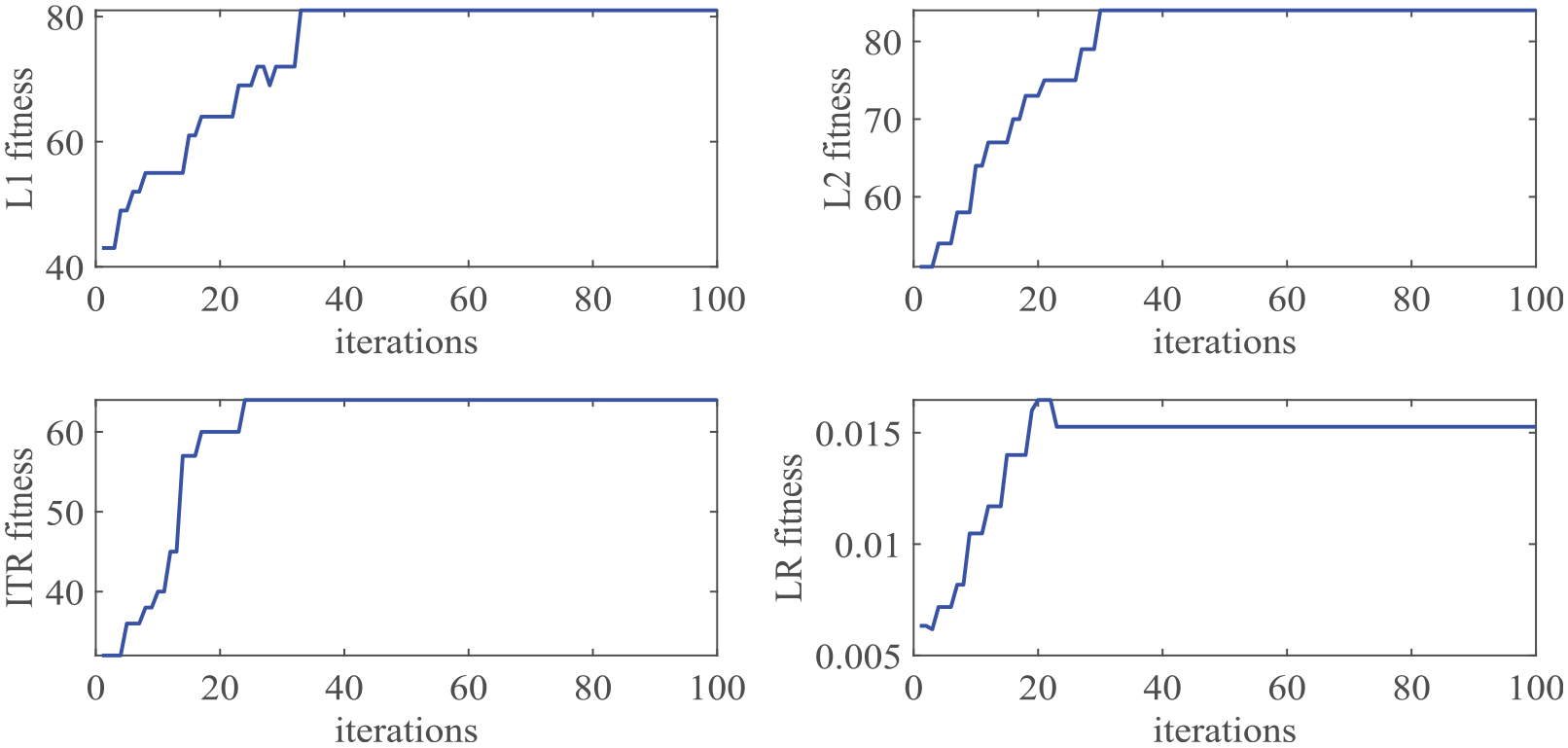
Fitness of hyper-parameters in LSTM network based on ISSA (dataset 2).

Table 2.

The optimized results.

Parameter	Optimal value (dataset 1)	Optimal value (dataset 2)
L1	98	81
L2	76	84
ITR	61	64
LR	7.2651e−03	15.2651e−03

This study selects the following five models for comparison to demonstrate the effectiveness of the proposed model. These models include ARIMA (Li et al., 2022), SVM (Yu et al., 2023), improved flower pollination algorithm optimized echo state network (IFPA-ESN) (Tang et al., 2021), PSO-LSTM (Zhao et al., 2024), and SSA-LSTM. For fair comparison, the parameters of these models are obtained through classical methods or methods introduced in the literature. For ARIMA, the AIC criterion is used to determine the order of the model. For SVM, the cross validation method class is used to determine the hyper-parameters of the model. For IFPA-ESN, the population size is 20, maximum number of iterations is 100, transition probability is 0.8, beta is 1.5, then IFPA is used to optimize ESN. For PSO-LSTM, the population size is 20, maximum number of iterations is 100, the weight coefficient is 0.8, and the acceleration factors are 2 and 1.5, PSO is used to optimize LSTM. For SSA-LSTM, the parameters are same with ISSA. The parameters of the 5 models are shown in Table 3.

Table 3.

The parameters of comparison models.

Model	Parameter (dataset 1)	Parameter (dataset 2)
ARIMA	p = 4, d = 2, q = 3	p = 3, d = 1, q = 3
SVM	c = 26.3306, g = 7.8059	c = 11.4239, g = 13.7006
IFPA-ESN	SR = 0.85, SD = 0.76, IS = 0.82, N = 76	SR = 0.88, SD = 0.77, IS = 0.81, N = 86
PSO-LSTM	L1 = 75, L2 = 67, ITR = 90, LR = 0.0073	L1 = 80, L2 = 72, ITR = 88, LR = 0.0076
SSA-LSTM	L1 = 84, L2 = 72, ITR = 92, LR = 0.0116	L1 = 81, L2 = 62, ITR = 68, LR = 0.0165

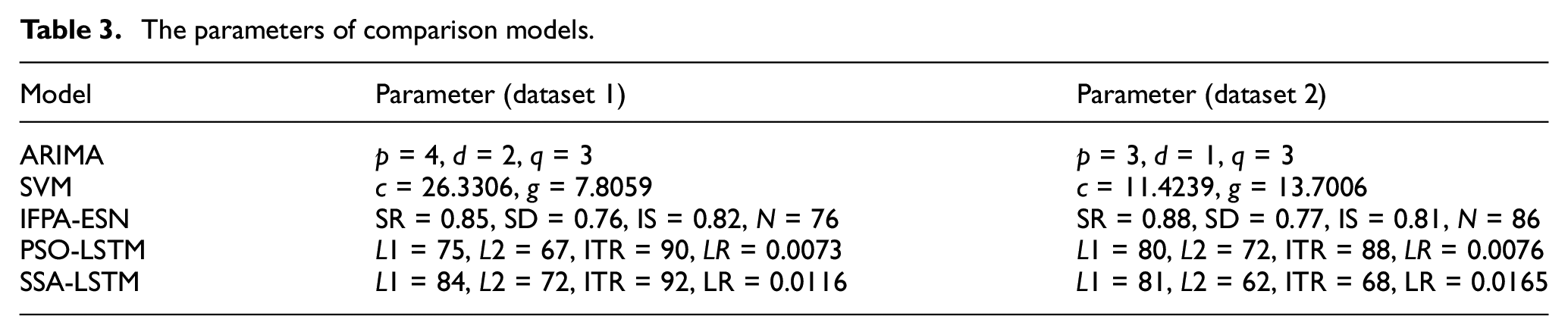
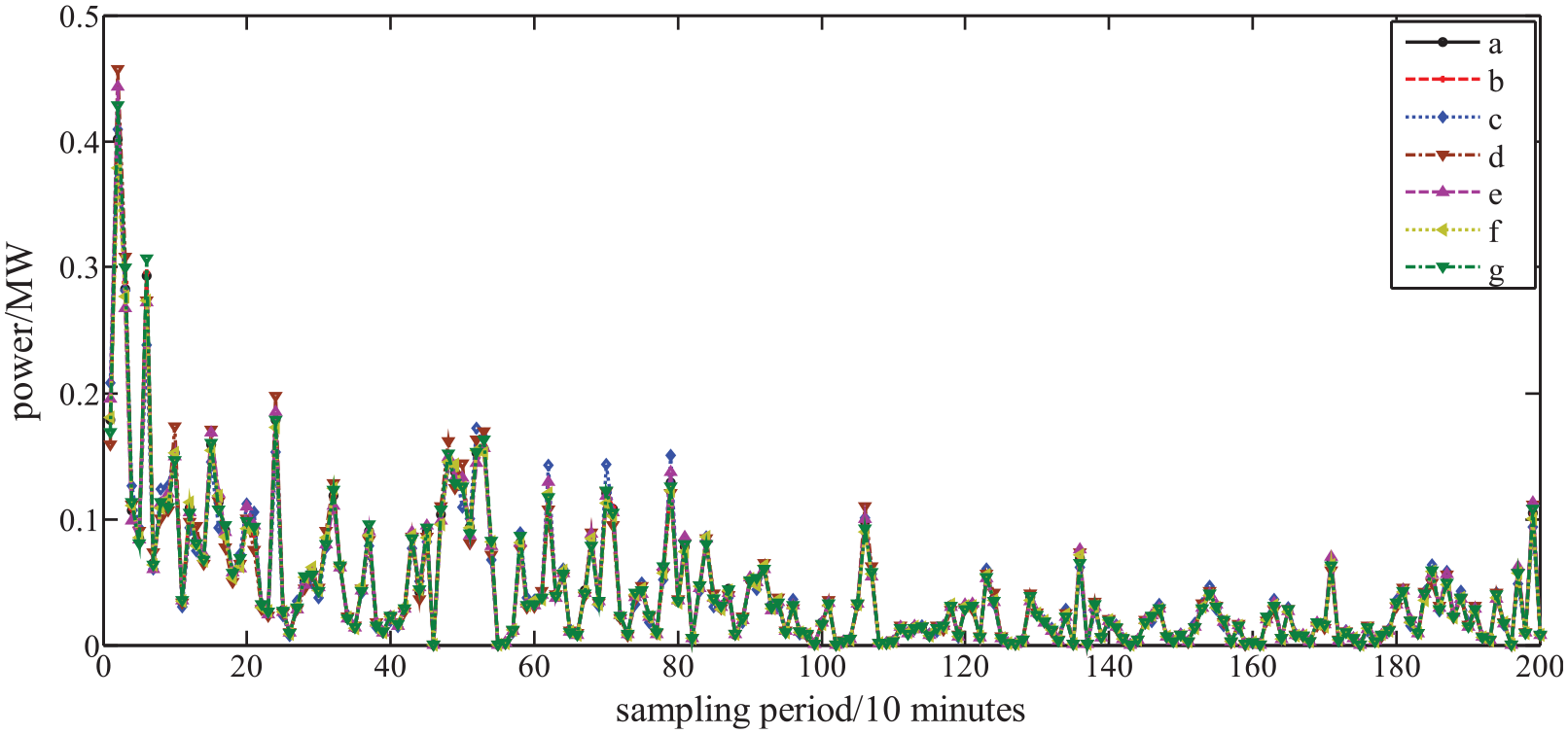
The ISSA optimized the parameters of the LSTM network and obtained the optimal values of four parameters. The optimized LSTM network was used to predict short-term wind power and obtain the final prediction result. The comparison curve between the predicted value and the actual value is shown in Figures 8 and 9. From the comparison results of the two graphs above, it can be seen that compared with the other five models, the ISSA-LSTM model can more accurately match the actual output and has better predictive performance compared to other models. The predicted values provided by this prediction method can more accurately reflect the actual short-term wind power.

Figure 8.

Short-term wind power prediction of each model for dataset 1 ((a): actual value; (b): proposed model; (c): ARIMA; (d) SVM; (e) IFPA-ESN; (f) PSO-LSTM; (g) SSA-LSTM).

Figure 9.

Short-term wind power prediction of each model for dataset 2 ((a) actual value, (b) proposed model, (c) ARIMA, (d) SVM, (e) IFPA-ESN, (f) PSO-LSTM, and (g) SSA-LSTM).

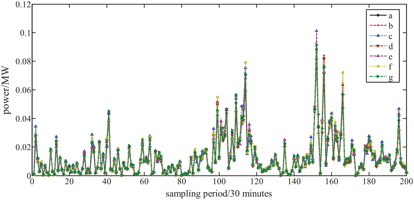
In order to observe the effectiveness of the proposed prediction model more intuitively, the prediction errors of each model for dataset 1 are shown in Figure 10, and the prediction errors for dataset 2 are shown in Figure 11. From Figure 10, it can be observed that the proposed prediction model has a smaller overall prediction error range, between [−0.0052, 0.0036]. Moreover, the fluctuation of errors during the prediction process is smaller compared to other models, and the prediction effect is more stable. The prediction error range of ARIMA is [−0.0290, 0.0549], and the prediction effect is poor. The error of SVM is basically between [−0.0552, 0.0200], and the error range of IFPA-ESN is basically within [−0.0415, 0.0209]. Although PSO-LSTM and SSA-LSTM have good stability performance, they have certain disadvantages in terms of stability and prediction accuracy compared to the proposed prediction models. From Figure 11, it can be observed that although the proposed model has some fluctuations in error, the overall error range is still far superior to other models, and the prediction accuracy also has a certain advantage. The prediction error range of the proposed model is mostly between [−0.0052, 0.0036], and the stability performance is good. In summary, the proposed model has certain advantages in stability and prediction accuracy.

Figure 10.

Prediction errors of each model for dataset 1 ((a) proposed model, (b) ARIMA, (c) SVM, (d) IFPA-ESN, (e) PSO-LSTM, and (f) SSA-LSTM).

Figure 11.

Prediction errors of each model for dataset 2 ((a) proposed model, (b) ARIMA, (c) SVM, (d) IFPA-ESN, (e) PSO-LSTM, and (f) SSA-LSTM).

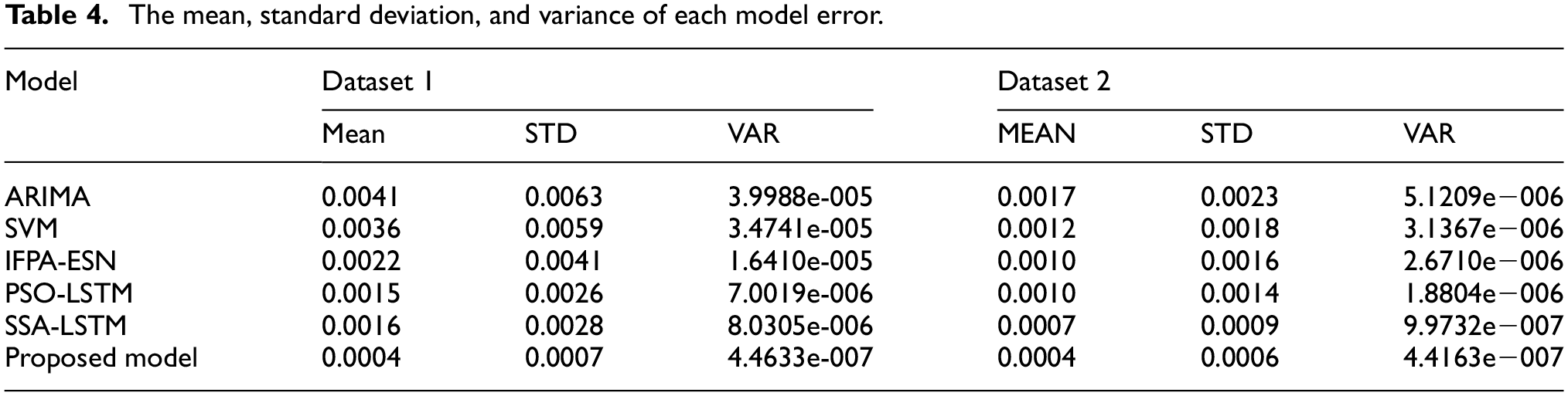
The mean value can reflect the concentration trend of model fitting errors, the standard deviation (STD) can reflect the degree of dispersion of fitting errors, and the variance (VAR) can reflect the fluctuation and stability of fitting errors. To avoid offsetting positive and negative errors, the absolute value of the error is used for calculation. Table 4 shows the mean, standard deviation, and variance of each model error.

Table 4.

The mean, standard deviation, and variance of each model error.

Model	Dataset 1			Dataset 2
Model	Mean	STD	VAR	MEAN	STD	VAR
ARIMA	0.0041	0.0063	3.9988e-005	0.0017	0.0023	5.1209e−006
SVM	0.0036	0.0059	3.4741e-005	0.0012	0.0018	3.1367e−006
IFPA-ESN	0.0022	0.0041	1.6410e-005	0.0010	0.0016	2.6710e−006
PSO-LSTM	0.0015	0.0026	7.0019e-006	0.0010	0.0014	1.8804e−006
SSA-LSTM	0.0016	0.0028	8.0305e-006	0.0007	0.0009	9.9732e−007
Proposed model	0.0004	0.0007	4.4633e-007	0.0004	0.0006	4.4163e−007

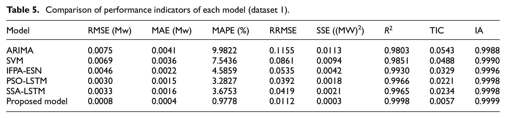
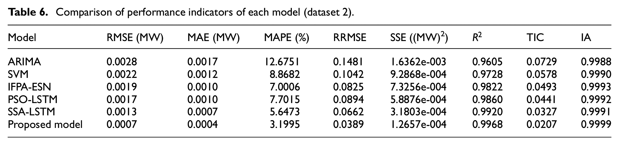
For the performance indicators used, the comparison results of dataset 1 are shown in Table 5. Similarly, the comparison results of dataset 2 are shown in Table 6. According to Table 5, it can be observed that the RMSE, MAE, MAPE, RRMSE, SSE, and TIC performance indicators of the proposed prediction model are all lower than the corresponding comparison models. Meanwhile, the IA and R² of the proposed model are closer to 1. Overall, the proposed model has significant advantages in both prediction performance and fit. By observing Table 6, it can be seen that the performance indicators of the proposed prediction model also have advantages. Therefore, these performance indicators can prove that the proposed prediction model is an effective solution to the short-term wind power prediction problem.

Table 5.

Comparison of performance indicators of each model (dataset 1).

Model	RMSE (Mw)	MAE (Mw)	MAPE (%)	RRMSE	SSE ((MW)²)	$R^{2}$	TIC	IA
ARIMA	0.0075	0.0041	9.9822	0.1155	0.0113	0.9803	0.0543	0.9988
SVM	0.0069	0.0036	7.5436	0.0861	0.0094	0.9851	0.0488	0.9990
IFPA-ESN	0.0046	0.0022	4.5859	0.0535	0.0042	0.9930	0.0329	0.9996
PSO-LSTM	0.0030	0.0015	3.2827	0.0392	0.0018	0.9966	0.0221	0.9998
SSA-LSTM	0.0033	0.0016	3.6753	0.0419	0.0021	0.9965	0.0234	0.9998
Proposed model	0.0008	0.0004	0.9778	0.0112	0.0003	0.9998	0.0057	0.9999

Table 6.

Comparison of performance indicators of each model (dataset 2).

Model	RMSE (MW)	MAE (MW)	MAPE (%)	RRMSE	SSE ((MW)²)	$R^{2}$	TIC	IA
ARIMA	0.0028	0.0017	12.6751	0.1481	1.6362e-003	0.9605	0.0729	0.9988
SVM	0.0022	0.0012	8.8682	0.1042	9.2868e-004	0.9728	0.0578	0.9990
IFPA-ESN	0.0019	0.0010	7.0006	0.0825	7.3256e-004	0.9822	0.0493	0.9993
PSO-LSTM	0.0017	0.0010	7.7015	0.0894	5.8876e-004	0.9860	0.0441	0.9992
SSA-LSTM	0.0013	0.0007	5.6473	0.0662	3.1803e-004	0.9920	0.0327	0.9991
Proposed model	0.0007	0.0004	3.1995	0.0389	1.2657e-004	0.9968	0.0207	0.9999

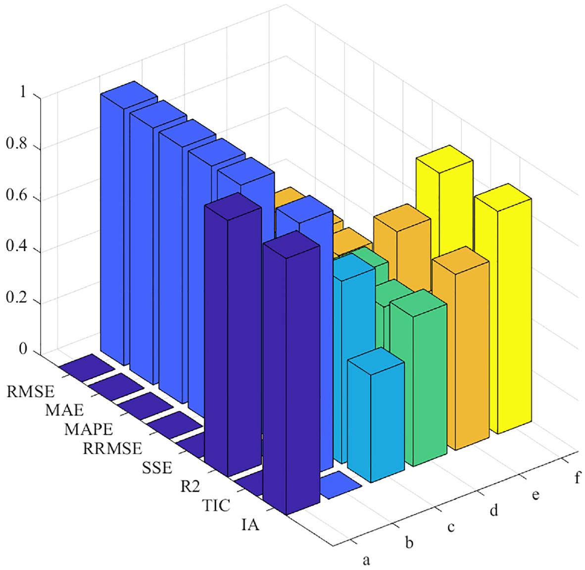
For a more intuitive comparison, Figures 12 and 13 show a comparison of the performance indicators of these prediction models (for the convenience of display, all performance indicators have been normalized to [0, 1]). Based on the above results in Tables and Figures, it can be concluded that the proposed ISSA-LSTM has better specific performance.

Figure 12.

Performance indicators of each model for dataset 1 ((a) proposed model, (b) ARIMA, (c) SVM, (d) IFPA-ESN, (e) PSO-LSTM, and (f) SSA-LSTM).

Figure 13.

Performance indicators of each model for dataset 2 ((a) proposed model, (b) ARIMA, (c) SVM, (d) IFPA-ESN, (e) PSO-LSTM, and (f) SSA-LSTM).

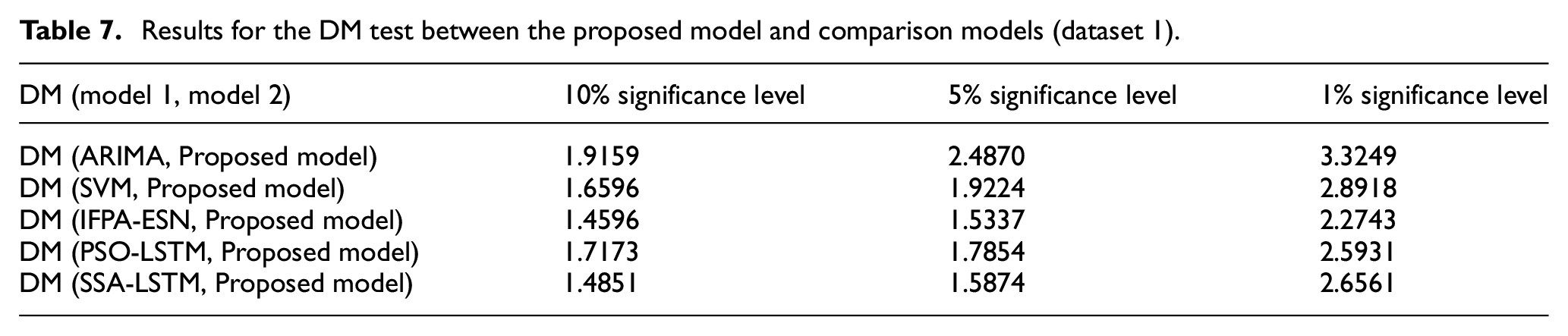
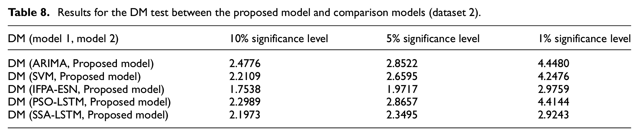
The DM test values of these prediction models with three typical significance levels are calculated and listed in Tables 7 and 8. From the results in Tables 7 and 8, it can be seen that the DM test values between the proposed prediction model and other models are all greater than 0. From this, it can be concluded that the proposed predictive model is significantly superior to other predictive models at different levels of significance.

Table 7.

Results for the DM test between the proposed model and comparison models (dataset 1).

DM (model 1, model 2)	10% significance level	5% significance level	1% significance level
DM (ARIMA, Proposed model)	1.9159	2.4870	3.3249
DM (SVM, Proposed model)	1.6596	1.9224	2.8918
DM (IFPA-ESN, Proposed model)	1.4596	1.5337	2.2743
DM (PSO-LSTM, Proposed model)	1.7173	1.7854	2.5931
DM (SSA-LSTM, Proposed model)	1.4851	1.5874	2.6561

Table 8.

Results for the DM test between the proposed model and comparison models (dataset 2).

DM (model 1, model 2)	10% significance level	5% significance level	1% significance level
DM (ARIMA, Proposed model)	2.4776	2.8522	4.4480
DM (SVM, Proposed model)	2.2109	2.6595	4.2476
DM (IFPA-ESN, Proposed model)	1.7538	1.9717	2.9759
DM (PSO-LSTM, Proposed model)	2.2989	2.8657	4.4144
DM (SSA-LSTM, Proposed model)	2.1973	2.3495	2.9243

The training and prediction times of each model for two datasets are shown in Table 9 (conducted 20 experiments and took the mean as the result). The configuration information of the simulation computer is as follows: CPU is Intel(R) Core(TM) i5-7300HQ CPU @ 2.50 GHz(2501 MHz), Memory is 8.00 GB (2400 MHz), Graphics card is NVIDIA GeForce GTX 1050 (4095 MB), simulation software is Matlab with version 2018b, operating system is Microsoft Windows 10 professional edition (64 bit). From the Table 9, it can be seen that PSO-LSSVM has the longest training time, followed by IFPA-LSTM, SSA-LSTM, and the time of the model in this paper is relatively close. The ARIMA model has the shortest time, followed by SVM. Although the training time of SVM and ARIMA is less than that of the proposed model, the prediction accuracy is far inferior to the proposed model. Although IFPA-LSTM and SSA-LSTM have certain advantages in terms of time consumption, their fitting degree with the true value curve is poor, and their stability is not as good as the model proposed in this paper. Although the model proposed in this article has a slightly longer prediction time, it fully meets the requirements compared to the sampling period and achieves good prediction results. For predicting time, there is not much difference among all models.

Table 9.

Training and prediction time of each model.

Model	Dataset 1		Dataset 2
Model	Training (minutes)	Prediction (seconds)	Training (minutes)	Prediction (seconds)
ARIMA	0.6235	6.3822	0.5903	0.5735
SVM	5.7732	9.3248	5.6442	5.6438
IFPA-ESN	7.3635	7.8220	7.4276	7.3999
PSO-LSTM	9.4556	6.3761	9.2673	9.2473
SSA-LSTM	6.3804	5.6906	5.5536	5.5300
Proposed model	6.2405	5.4264	5.3747	5.4153

Based on the data fitting curve, prediction error, performance indicators, DM test, and the time required for the model, it can be seen that the proposed model has achieved the best prediction results compared to other models, proving that the proposed model is reliable and effective.

Conclusions

A prediction model was proposed and validated for short-term wind power prediction in this paper. An improved LSTM model has been proposed. Compared with traditional LSTM, each gate of the new LSTM can “peek” at the unit state, improving prediction accuracy. On the basis of the standard SSA, an ISSA is proposed by combining various strategies such as Cauchy mutation optimization, opposition-based learning and dynamic weighting to optimize the hyper-parameters of the LSTM network. Predict short-term wind speed through optimized LSTM. The performance of the model is validated through two sets of actual collected short-term wind power data. Compared with other models, multiple validation methods have demonstrated the excellent performance of the proposed prediction model, which is very suitable for practical wind farms.

Although the ISSA algorithm obtained the optimal hyper-parameters of LSTM in the experiment, which further improved the prediction results, there is still a problem of wasting a lot of time in the optimization process of the ISSA. In the future, reasonable trade-offs should be made or SSA should be further improved to seek a reasonable balance between computation time and prediction accuracy.

Footnotes

Declaration of conflicting interests

The author declared no potential conflicts of interest with respect to the research, authorship, and/or publication of this article.

Funding

The author disclosed receipt of the following financial support for the research, authorship, and/or publication of this article: This paper is supported by the Science Research Project of Liaoning Education Department (No. LJKZ0145).

ORCID iD

Fei Tang

Data availability statement

The data used to support the results of this study can be obtained from the corresponding author

References

Awadallah

Al-Betar

Doush

, et al. (2023) Recent versions and applications of sparrow search algorithm. Archives of Computational Methods in Engineering 30, 5: 2831–2858.

Cai

Dai

Ding

, et al. (2023) Gray wolf optimization-based wind power load mid-long term forecasting algorithm. Computers & Electrical Engineering 109: 108769.

Dong

Dou

, et al. (2022) Optimization of capacity configuration of wind–solar–diesel–storage using improved Sparrow Search algorithm. Journal of Electrical Engineering and Technology 17: 1–14.

Duan

Wang

, et al. (2022) A novel hybrid model based on nonlinear weighted combination for short-term wind power forecasting. International Journal of Electrical Power & Energy Systems 134: 107452.

Zhang

Shao

, et al. (2023) A short-term prediction model of wind power with outliers: An integration of long short-term memory, ensemble empirical mode decomposition, and sample entropy. Sustainability 15: 6285.

Geng

Sun

Wang

, et al. (2023) A modified adaptive sparrow search algorithm based on chaotic reverse learning and spiral search for global optimization. Neural Computing and Applications 35: 24603–24620.

Hou

Jiang

Luo

, et al. (2024) Dynamic path planning for mobile robots by integrating improved sparrow search algorithm and dynamic window approach. Actuators 13: 24.

Ishikawa

Kojima

Namerikawa

(2017) Short-term wind power prediction for wind turbine via Kalman filter based on JIT modeling. Electrical Engineering in Japan 198(3): 86–96.

Jing

Zhao

(2023) A data expansion based piecewise regression strategy for incrementally monitoring the wind turbine with power curve. Journal of Central South University 30(5): 1601–1617.

10.

Kari

Guoliang

Kesong

, et al. (2023) Short-term wind power prediction based on combinatorial neural networks. Intelligent Automation & Soft Computing 37: 1437–1452.

11.

Khasanzoda

Zicmane

Beryozkina

, et al. (2022) Regression model for predicting the speed of wind flows for energy needs based on fuzzy logic. Renewable Energy 191: 723–731.

12.

Klaiber

Van Dinther

(2024) Deep learning for variable renewable energy: A systematic review. ACM Computing Surveys 56(1): 1–37.

13.

Yang

Miao

, et al. (2023a) An adaptive spatiotemporal fusion graph neural network for short-term power forecasting of multiple wind farms. Journal of Renewable and Sustainable Energy 15(1): 013310.

14.

Liu

, et al. (2024a) Thermal error prediction of precision boring machine tools based on extreme gradient boosting algorithm-improved sailed fish optimizer-bi-directional ordered neurons-long short-term memory neural network model and physical-edge-cloud system. Engineering Applications of Artificial Intelligence 127: 107278.

15.

Yang

, et al. (2024b) Short-term wind power forecast based on continuous conditional random field. IEEE Transactions on Power Systems 39(1): 2185–2197.

16.

Liu

, et al. (2023b) Ultra-short-term wind power forecasting based on deep Bayesian model with uncertainty. Renewable Energy 205: 598–607.

17.

Liu

Fang

, et al. (2023a) The recursive grey model and its application. Applied Mathematical Modelling 119: 447–464.

18.

Liu

Tan

Yuan

, et al. (2022) Combination weighting-based method for access point optimization of offshore wind farm. Energy Reports 8: 900–907.

19.

Zhang

(2014) Study on short-term wind power prediction model based on ARMA theory. In: International conference on renewable energy and environmental technology, 2013, pp.1875–1878. New York: IEEE.

20.

Sabas

Mendez

(2022) Wind energy forecasting using multiple ARIMA models. In: IEEE international conference on automation science and engineering, 2022, pp.2034−2039.

21.

Niksa-Rynkiewicz

Stomma

Witkowska

, et al. (2023) An intelligent approach to short-term wind power prediction using deep neural networks. Journal of Artificial Intelligence and Soft Computing Research 13(3): 197–210.

22.

Priyadarshi

Bhaskar

Almakhles

(2024) A novel hybrid whale optimization algorithm differential evolution algorithm-based maximum power point tracking employed wind energy conversion systems for water pumping applications: Practical realization. IEEE Transactions on Industrial Electronics 71(2): 1641–1652.

23.

Qin

Huang

Wang

, et al. (2023) Ultra-short-term wind power prediction based on double decomposition and LSSVM. Transactions of the Institute of Measurement and Control 45: 2627–2636.

24.

Saeed

Ibrahim

El-Kenawy

ESM

, et al. (2023) Forecasting wind power based on an improved al-Biruni Earth radius metaheuristic optimization algorithm. Frontiers in Energy Research 11: 1220085.

25.

Saini

Kumar

Al-Sumaiti

, et al. (2023) Learning based short term wind speed forecasting models for smart grid applications: An extensive review and case study. Electric Power Systems Research 222: 109502.

26.

Sun

, et al. (2014) An investigation of the persistence property of wind power time series. Science China Technological Sciences 57: 1578–1587.

27.

Sun

Jin

, et al. (2023) Spatiotemporal wind power forecasting approach based on multi-factor extraction method and an indirect strategy. Applied Energy 350: 121749.

28.

Tang

Zhao

Ouyang

(2021) Two-phase deep learning model for short-term wind direction forecasting. Renewable Energy 173: 1005–1016.

29.

Wang

(2023) Wind speed interval prediction based on multidimensional time series of convolutional neural networks. Engineering Applications of Artificial Intelligence 121: 105987.

30.

Wei

Yang

, et al. (2023) Ultra-short-term forecasting of wind power based on multi-task learning and LSTM. International Journal of Electrical Power & Energy Systems 149: 109073.

31.

Wei

Zhang

Song

, et al. (2024) Research on evacuation path planning based on improved Sparrow Search algorithm. Computer Modeling in Engineering and Sciences 139: 1295–1316.

32.

Xue

Shen

(2020) A novel swarm intelligence optimization approach: Sparrow search algorithm. Systems Science & Control Engineering 8(1): 22–34.

33.

Zhang

Chen

, et al. (2023) A deep learning framework for day ahead wind power short-term prediction. Applied Sciences 13: 4042.

34.

Yue

Cao

, et al. (2023) Review and empirical analysis of sparrow search algorithm. Artificial Intelligence Review 56: 10867–10919.

35.

Meng

Pau

, et al. (2023) Research on hierarchical control strategy of ESS in distribution based on GA-SVR wind power forecasting. Energies 16: 2079–2079.

36.

Zeng

Lan

Wang

, et al. (2023) Short-term wind power prediction based on the combination of numerical weather forecast and time series. Journal of Renewable and Sustainable Energy 15(1): 013303.

37.

Zhang

Yang

Qin

, et al. (2022) A multi-strategy improved sparrow search algorithm for solving the node localization problem in heterogeneous wireless sensor networks. Applied Sciences 12: 5080.

38.

Zhang

Zhao

, et al. (2023) Deterministic and probabilistic prediction of wind power based on a hybrid intelligent model. Energies 16: 4237.

39.

Zhao

Guo

, et al. (2024) Short-term wind power prediction based on combined long short-term memory. IET Generation Transmission & Distribution 18: 931–940.

40.

Zheng

Jin

(2022) A reliable method of wind power fluctuation smoothing strategy based on multidimensional non-linear exponential smoothing short-term forecasting. IET Renewable Power Generation 16(16): 3573–3586.