Short-term wind power forecasting for newly constructed wind farms using transfer learning-based LSTM-GRU models

Abstract

As a critical technology for enhancing wind energy utilization efficiency, wind power forecasting requires extensive historical data for high-accuracy models. Addressing data scarcity in new wind farms, this study proposes a transfer learning-based LSTM-GRU hybrid model. An optimal feature window preserved temporal dynamics and suppressed redundant noise within a multidimensional feature matrix. The cross-domain framework employs LSTM in data-rich source domains and lightweight GRU in data-scarce targets. Source-domain LSTM parameters transfer to enhance temporal modeling, with transferred layers frozen and only GRU layers fine-tuned, balancing knowledge transfer and domain adaptation. Experimental results show the proposed transfer method reduced MAE by 18.8% and 34.5%, and RMSE by 19.0% and 32.1%, outperforming conventional single-domain models. Freezing transferred parameters decreased trainable parameters, accelerating convergence speed by 26.9% and 17.9%. This study offers managerial support for efficient new wind farm commissioning, improved grid dispatch, and more reliable investment decisions.

Keywords

wind power forecasting transfer learning newly constructed wind farms LSTM-GRU optimal temporal feature window

Introduction

Amid increasing pressure from global climate change and the continuous depletion of fossil fuel reserves, wind energy has emerged as a vital clean energy source due to its technological maturity and cost-effectiveness (Wang et al., 2024). Consequently, countries worldwide are actively developing new wind farm projects to harness wind potential and meet growing energy demands. However, the intermittency and variability of wind power generation pose significant challenges to grid stability. Therefore, accurate wind power forecasting is critical for reliable grid dispatch and operations (Wang et al., 2021; Zhao et al., 2025).

Early wind power forecasting methods were primarily based on physical models and statistical approaches (Wang et al., 2023). Physical models, often centered on Numerical Weather Prediction (NWP), first predict wind speed by combining NWP with the actual terrain and geographical conditions of a wind farm and then determine the power output (Hu et al., 2021; Khalid and Savkin, 2012) constructed power curve models by inputting NWP data, such as wind speed, temperature, and air pressure. El-Fouly et al. (2006) obtained predicted values by establishing differential equation models through cumulative processing of raw data. These methods offer clear physical interpretations and do not require historical data, but they depend heavily on NWP accuracy and involve complex computations. Moreover, terrain modeling errors can accumulate, and their effectiveness for short-term forecasting is often insufficient due to timeliness constraints.

Statistical methods establish mathematical relationships between inputs (e.g., wind speed and meteorological parameters) and outputs (power) based on historical data. In time series analysis, the Autoregressive Integrated Moving Average (ARIMA) model handles stationary sequences through differencing and linear combinations (Lydia et al., 2016). The Kalman filter utilizes dynamic state-space models to update predictions in real time (Xiu and Guo, 2013). Regression analysis employs linear or nonlinear equations to fit the wind-speed-to-power relationship, while the persistence method uses the current power value directly as the future forecast. Do et al. (2016) applied the ARMA model, employing data transformation and standardization, to simulate and predict the hourly average wind speed for Jeju Island, South Korea, using data from 2010 to 2012. These statistical methods are computationally simple and well-suited for short-term forecasting, but they require identifying statistical patterns within historical data. Their performance depends critically on data quality; for newly constructed wind farms lacking sufficient data, the predictive effectiveness of statistical models declines significantly.

In recent years, advancements in artificial intelligence and big data technologies, wind power forecasting has gradually shifted from traditional methods to data-driven intelligent models. Representative machine learning models include support vector machines (SVM), decision trees, random forests (Lahouar and Ben Hadj Slama, 2017), and K-means clustering (Azimi et al., 2016). Li et al. (2022) proposed an improved least squares support vector machine (LSSVM) model combined with ensemble empirical mode decomposition (EEMD) and a Tent-chaotic-map-optimized sparrow search algorithm (SSA), constructing a hybrid framework for wind power forecasting. Hu et al. (2025) developed an ultra-short-term forecasting method for mountainous wind farms, which selects critical turbine features through random forests and the maximal information coefficient. The method integrates time finite difference (TFD) with autoregressive structures to build AR-TFD-ML and PWARX-TFD-ML models for multi-step wind condition forecasting and dynamic wind farm modeling, employing kernel density estimation to quantify predictive uncertainty. While effective in improving forecasting accuracy, such methods suffer from high model complexity and computational cost. More generally, machine learning-based forecasting often relies on feature extraction and enhancement to supplement temporal features, which inevitably increases computational burden and time consumption.

With the advancement of deep learning, deep neural network-based approaches have emerged as the mainstream. These include recurrent neural networks (RNN), convolutional neural networks (CNN) (Jalali et al., 2022), temporal convolutional networks (TCN) (Nguyen et al., 2023), and Transformer-based architectures, often enhanced by optimization algorithms to improve accuracy. Mei et al. (2024) proposed the MLL-MPFLA model that integrates a multilayer perceptron with an LSTM encoder–decoder, introducing a multi-point focused linear attention mechanism in the decoding stage to jointly capture multidimensional and temporal features, thereby enhancing short-term forecasting accuracy. Yang et al. (2025) developed a short-term forecasting method that considers wind speed shift. Their approach uses a directed acyclic graph to identify shift scenarios, WGAN-GP for data augmentation, and a TCN with multi-head attention to improve accuracy. Although effective, this method remains computationally expensive. Liu et al. (2021) introduced a short-term forecasting model based on stacked recurrent neural networks (SRNN) with a parameterized sine activation function (PSAF), where trainable sine functions replace conventional monotonic activation functions to better capture nonlinear temporal features. However, the model’s parameter sensitivity analysis relies solely on grid search, lacking automated hyperparameter optimization and thus limiting efficiency.

Nevertheless, when applied to newly built wind farms, the aforementioned models face a critical challenge: they typically require large amounts of historical operational data for training. At the early stage of operation, data scarcity severely restricts the model’s learning capacity, leading to weakened generalization ability and unstable forecasting accuracy, which directly affect the reliability and economic optimization of wind farm operation.

To address the data scarcity issue in newly built wind farms, several approaches have been proposed. These include data augmentation using generative adversarial networks (GAN) (Meng et al., 2022) and cross-farm data sharing (Liao et al., 2023), which construct multi-source data-driven frameworks and leverage the feature extraction capability of deep neural networks to enhance forecasting accuracy under limited-sample scenarios. Liu et al. (2024) proposed a Bayesian deep learning-based adaptive wind power forecasting method (BDL-AWFPP), which fuses CFD simulation results with turbine power curves to build multi-source prior datasets. This method achieves high accuracy even in the absence of sufficient operational data, but its computational complexity is high and its performance heavily depends on the quality of prior data and numerical weather prediction (NWP). Yin et al. (2025) proposed the SDM-VMD-IENN model, which alleviates negative transfer through similarity-based data matching, reduces nonlinear complexity using variational mode decomposition (VMD), and enhances predictive stability via evolutionary neural network optimization of multi-loss functions. However, this model heavily relies on the availability of sufficiently similar source domain data, limiting its applicability.

Confronting scarce training data, this study adopts transfer learning as the theoretical foundation for accuracy enhancement by supplementing data insufficiency through parameter transfer, selecting a combined Long Short-Term Memory (LSTM) and Gated Recurrent Unit (GRU) architecture. The main reasons are as follows: LSTM—as a Recurrent Neural Network (RNN) variant—effectively captures long-term dependencies in time series via three gating mechanisms; GRU simplified structure reduces parameters, lowering computational complexity while improving training efficiency and performance; both models offer stackable flexibility for adjusting depth and width to accommodate varying data scales; compared to CNNs, the LSTM-GRU combination eliminates fixed-size receptive field dependencies, adaptively modeling non-stationary wind power sequences and handling spiky fluctuations under abrupt wind changes; versus traditional machine learning methods like SVM, it autonomously learns nonlinear mappings between meteorological factors and power output through gating units without manual feature engineering, significantly enhancing multi-sensor data fusion; relative to Transformers, this solution demonstrates superior positional encoding independence and computational efficiency, achieving robust domain adaptation without large-scale pretraining when processing wind farm data.

Consequently, this study proposes a transfer learning-based LSTM-GRU hybrid model for wind power forecasting that mitigates overfitting and underfitting caused by scarce training data in newly constructed wind farms, thereby enhancing forecasting accuracy. The proposed method enables accurate power forecasting from the inception of a new wind farm’s operation, thereby reducing operational risks, enhancing grid integration, and supporting strategic investment decisions—ultimately accelerating the sustainable deployment of wind energy.

The contributions of this paper are as follows:

(1) An investigation is conducted into the correlation between input feature window length and forecasting accuracy in wind power forecasting models, with multiple time-series training samples constructed via sliding window techniques to determine the optimal historical data feature window.

(2) The LSTM model undergoes pre-training on the source-domain dataset (historical data-rich wind farms), where comprehensive learning of temporal features enables the capture of nonlinear mappings between diverse input characteristics and electrical power output.

(3) A heterogeneous LSTM-GRU recurrent architecture is developed that leverages LSTM long-term memory and GRU structural efficiency. The LSTM layers preserve complex relational representations from source-domain pre-training, while newly added GRU layers provide flexibility for target-domain feature adaptation.

(4) During target-domain (new wind farms) fine-tuning, a layered parameter update strategy is implemented: frozen pre-trained LSTM parameters with exclusive optimization of GRU and fully-connected layers. This approach maintains transferred source-domain knowledge while enabling target-domain adaptation through localized parameter adjustment.

The remainder of this paper is structured as follows: the fundamental models section introduces fundamental LSTM and GRU models along with transfer learning theory; the section, transfer learning-based LSTM-GRU wind power forecasting model, specifies parameter selection methodology for the proposed model; the experiments section presents experimental results; and the conclusion section concludes with research findings while outlining future work directions.

Fundamental models

Long short-term memory networks

Compared to RNNs, the LSTM architecture incorporates three critical gating components—input gate, forget gate, and output gate—along with a memory cell state (denoted as C) that serves as a dedicated information retention pathway (Riedel et al., 2024).

The structure of the LSTM neuron is shown in Figure 1.

Figure 1.

LSTM cell architecture.

Upon input $x_{(t)}$ , The forget gate computes the discard ratio $f_{(t)}$ for cell state information:

f_{(t)} = σ (W_{x f}^{T} x_{(t)} + W_{h f}^{T} h_{(t - 1)} + b_{f})

(1)

Subsequently, the input gate calculates the new information ratio $i_{(t)}$ and generates candidate state $g_{(t)}$ :

i_{(t)} = σ (W_{x i}^{T} x_{(t)} + W_{h i}^{T} h_{(t - 1)} + b_{i})

(2)

g_{(t)} = \tanh (W_{x g}^{T} x_{(t)} + W_{h g}^{T} h_{(t - 1)} + b_{g})

(3)

The cell state $c_{(t)}$ is updated by combining these outputs:

{c_{(t)} = f}_{(t)} \otimes c_{(t - 1)} + i_{(t)} \otimes g_{(t)}

(4)

Finally, the output gate regulates the output ratio $o_{(t)}$ , and the hidden state $h_{(t)}$ is derived from the modulated cell state:

o_{(t)} = σ (W_{x o}^{T} x_{(t)} + W_{h o}^{T} h_{(t - 1)} + b_{o})

(5)

y_{(t)} = h_{(t)} = o_{(t)} \otimes \tanh (c_{(t)})

(6)

The output $y_{(t)} = h_{(t)}$ simultaneously serves dual roles: as the current timestep output and the next timestep input.

In all preceding equations, $W_{* *}^{T}$ denotes the gate weight matrices (where ∗ corresponds to f, i, g, o for forget, input, cell, and output gates respectively), $b_{*}$ signifies the gate bias terms, $h_{(t - 1)}$ and $h_{(t)}$ represent the previous and current hidden states, $σ$ indicates the Sigmoid activation function with output constrained to [0,1] where 0 signifies complete discarding and 1 denotes full retention.

Gated recurrent unit

The Gated Recurrent Unit (GRU) constitutes a streamlined variant of LSTM that structurally streamlines the original three gating mechanisms into two core components: an update gate and a reset gate (Zhao et al., 2023).

The structure of the GRU neuron is shown in Figure 2.

Figure 2.

GRU cell architecture.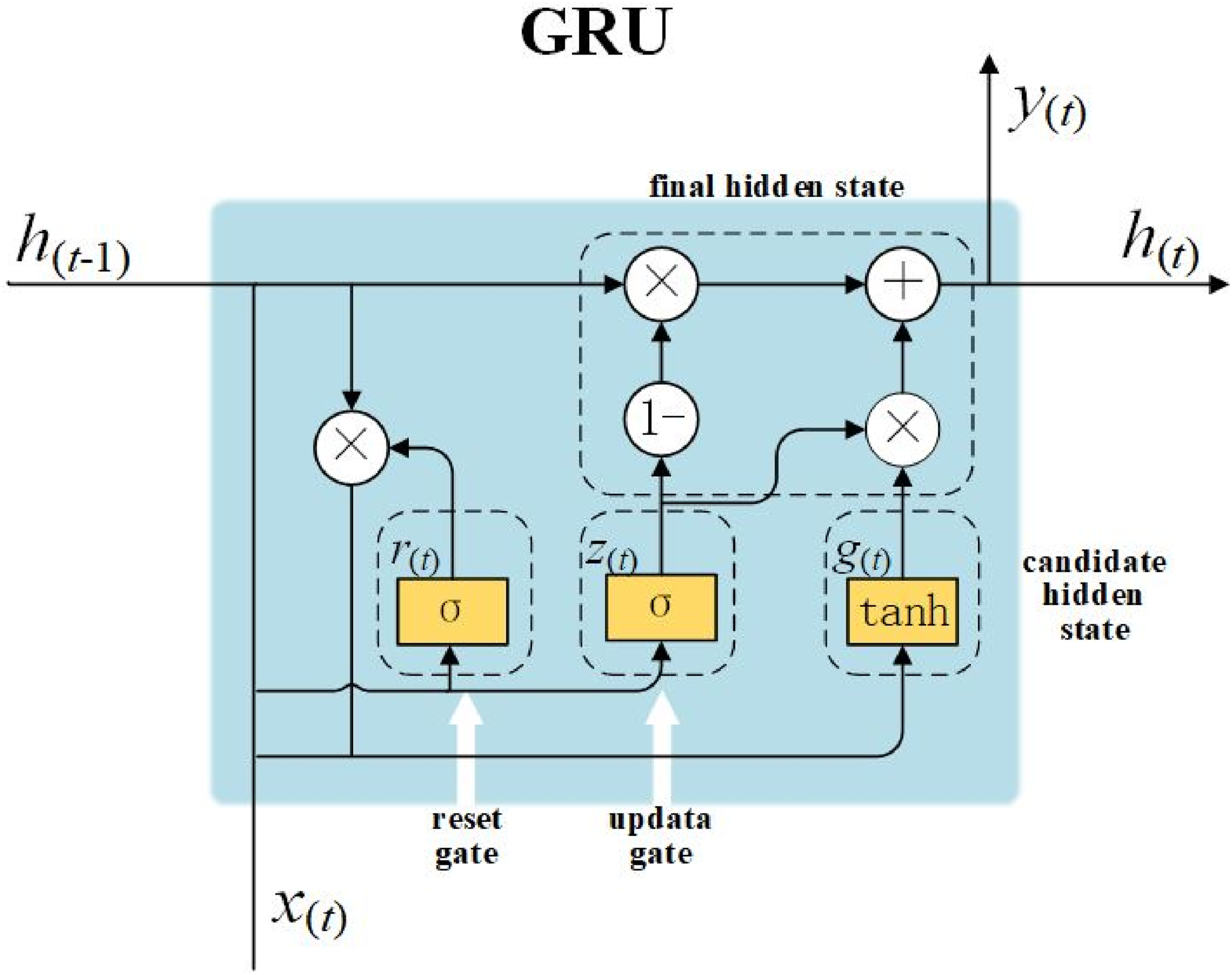

Upon input $x_{(t)}$ , the reset gate $r_{(t)}$ determines which informational components from the previous hidden state $h_{(t - 1)}$ should be discarded for candidate hidden state generation:

r_{(t)} = σ (W_{x r}^{T} x_{(t)} + W_{h r}^{T} h_{(t - 1)} + b_{r})

(7)

Subsequently, the update gate $z_{(t)}$ governs the retention ratio of historical states versus adoption of candidate features:

z_{(t)} = σ (W_{x z}^{T} x_{(t)} + W_{h z}^{T} h_{(t - 1)} + b_{z})

(8)

The intermediate candidate hidden state $g_{(t)}$ is then formulated by integrating current inputs with reset-gate-filtered historical states:

g_{(t)} = \tanh (W_{x g}^{T} x_{(t)} + W_{h g}^{T} (r_{(t)} \otimes h_{(t - 1)}) + b_{g})

(9)

Finally, the updated hidden state $h_{(t)}$ is derived by mediating legacy-new information fusion through $z_{(t)}$ :

y_{(t)} = h_{(t)} = (1 - z_{(t)}) \otimes h_{(t - 1)} + z_{(t)} \otimes g_{(t)}

(10)

Concurrently, the output $y_{(t)} = h_{(t)}$ serves dual roles: as current timestep output and subsequent timestep input.

In all preceding equations, $W_{* *}^{T}$ denotes the gate weight matrices, $b_{*}$ signifies the gate bias terms, $h_{(t - 1)}$ and $h_{(t)}$ represent the previous and current hidden states, $σ$ indicates the Sigmoid activation function with output constrained to [0,1] where 0 signifies complete discarding and 1 denotes full retention.

Transfer learning theory

Transfer Learning, a pivotal subfield of machine learning, fundamentally operates by transferring knowledge acquired in a Source Domain to a Target Domain, thereby overcoming conventional models’ strong dependency on same-source and same-distribution data (Lu et al., 2015). This methodology facilitates cross-domain knowledge representation transfer by exploiting latent correlations between distinct yet related domains, and is particularly applied in scenarios characterized by target-domain sample scarcity or significant distribution discrepancies.

In wind power forecasting research, conventional single-domain data-driven modeling approaches consequently confront generalization capability challenges due to scarce historical data in newly constructed wind farms. This study addresses this limitation by constructing a parameter-transfer-based deep neural network model that designates data-rich wind farms as the source-domain knowledge base.

f_{T} (x) = f_{shared} (x; θ_{shared}) + f_{specific} (x; θ_{T})

(11)

where

x

denotes the input feature data and

f_{T} (x)

represents the final output;

f_{shared} (x; θ_{shared})

signifies the shared submodel transferred from the source-domain task, with parameters

θ_{shared}

obtained from the source domain; and

f_{specific} (x; θ_{T})

corresponds to the task-specific component for the target domain, where parameters

θ_{T}

are derived from the target domain.

In this paper, we utilize the model parameter sharing mechanism in order to solve the typical problem of insufficient training samples due to the limited amount of data from wind farms.

Transfer learning-based LSTM-GRU wind power forecasting model

This section delineates the critical parameter selection methodology for the proposed model, elucidates information propagation at the LSTM-GRU network junction, and specifies implementation details of the cross-domain transfer framework.

Optimal temporal feature window

Since the output power of wind power systems is essentially an integrated quantity over time rather than an instantaneous observation, the power generation process exhibits significant temporal dependencies and nonlinear coupling characteristics (Zhao et al., 2024). The cumulative power generation during a given time period is not only directly influenced by the current meteorological conditions (including wind speed, wind direction, air pressure, etc.), but is also strongly correlated with the dynamic evolution trends of various driving factors within a historical time window (typically from time t-n to t).

In the process of temporal feature modeling, the choice of window length directly affects the model’s ability to capture the correlation between features and the target. A window that is too short may reduce computational complexity and shorten the training cycle, but it can lead to insufficient feature representation, making it difficult for the model to establish an effective feature-response mechanism. Conversely, an excessively long window may enhance the completeness of historical information, but it significantly increases the model’s capacity requirements and introduces redundant noise, thereby elevating the risk of overfitting.

Therefore, determining the optimal temporal feature window length is a critical step in experimental design for improving both the forecasting accuracy and computational efficiency of the model.

In the dataset, each data instance is structured as shown below.

D_{t} = [{{f e a t u r e_1}_{t}, f e a t u r e_2}_{t}, . . ., {f e a t u r e_n}_{t}, P_{t}]

(12)

F_{t} = [{{f e a t u r e_1}_{t}, f e a t u r e_2}_{t}, . . ., {f e a t u r e_n}_{t}]

(13)

Here, $D_{t}$ contains the n climatic features at time t along with the current power output $P_{t}$ , while $F_{t}$ represents the feature vector at time t, constructed by removing $P_{t}$ from $D_{t}$ .

When the window length is s and the target forecasting time is y, the constructed feature matrix is as follows:

X_{y}^{s \times n} = {[\begin{array}{l} {f e a t u r e_1}_{y - s} & {f e a t u r e_2}_{y - s} & \begin{array}{l} . . . . & {f e a t u r e_n}_{y - s} \end{array} \\ \begin{array}{l} {f e a t u r e_1}_{y - s + 1} \\ \begin{array}{l} . . . . \\ {f e a t u r e_1}_{y - 2} \end{array} \end{array} & \begin{array}{l} {f e a t u r e_2}_{y - s + 1} \\ \begin{array}{l} . . . . \\ {f e a t u r e_2}_{y - 2} \end{array} \end{array} & \begin{array}{l} \begin{array}{l} . . . . & {f e a t u r e_n}_{y - s + 1} \end{array} \\ \begin{array}{l} \begin{array}{l} . . . . \\ . . . . \end{array} & \begin{array}{l} . . . . \\ {f e a t u r e_n}_{y - 2} \end{array} \end{array} \end{array} \\ {f e a t u r e_1}_{y - 1} & {f e a t u r e_2}_{y - 1} & \begin{array}{l} . . . . & {f e a t u r e_n}_{y - 1} \end{array} \end{array}]}_{(s \times n)}

(14)

The feature matrix $X_{y}^{s \times n}$ corresponds to the target value $P_{y}$ .

By adjusting the window length to obtain the optimal feature window length on the source domain dataset, the model’s output can more closely approximate the true distribution of the observed data. The specific procedure is outlined in Figure 3. When selecting the optimal window length, it is not sufficient to consider only the value of R²; the training time required by the model must also be taken into account.

Figure 3.

Optimal feature window length selection.

Model structure selection

This section introduces the specific process for selecting the model structure used in this study.

Source domain model structure

LSTM models with different inter-layer structural configurations exhibit significant variations in their ability to fit data features. Specifically, hyperparameters such as the number of hidden layers and the number of neurons per layer adjust the model’s nonlinear fitting capability by altering its representational capacity. Therefore, it is necessary to systematically conduct comparative experiments to evaluate how network depth (number of hidden layers) and unit density (number of neurons per layer) impact model performance metrics, thereby determining the optimal combination of hidden layer architecture parameters. The specific procedure is outlined in Figure 4.

Figure 4.

Source model construction.

Connection points in heterogeneous models

LSTM and GRU are both types of recurrent neural networks. The output of each time step from the LSTM is directly used as the input to the GRU, as shown in the Figure 5.

Figure 5.

Model connection point.

The forward propagation at the connection point is described by the following equations (15) and (16):

h_{t}^{L S T M} = LSTM (x_{t}, h_{t - 1}^{L S T M}, c_{t - 1}^{L S T M})

(15)

h_{t}^{GRU} = GRU (h_{t}^{L S T M}, h_{t - 1}^{GRU})

(16)

Let the loss function be denoted as $L$ . The backpropagation is expressed by the following Equation.

\frac{\partial L}{\partial θ_{L S T M}} = 0 (θ_{L S T M} i s f r o z e n)

(17)

\frac{\partial L}{\partial θ_{GRU}} = \sum_{t = 1}^{T} \frac{\partial L}{\partial h_{t}^{GRU}} \cdot \frac{\partial h_{t}^{GRU}}{\partial θ_{GRU}}

(18)

Here, h represents the hidden states of each network, c denotes the memory cell in the LSTM, and θ refers to all trainable parameters of the model.

During forward propagation, the LSTM layer performs multi-level feature extraction on the input sequential data, generating a sequence of hidden states that capture long-term dependencies. The GRU units dynamically model temporal sequences by integrating the current LSTM output features with their own historical hidden states through a gating mechanism. The optimized temporal features are then passed to the fully connected layer.

During backpropagation, the gradient signals derived from the loss function are used to iteratively optimize the trainable parameters of the GRU layer via the backpropagation algorithm. The LSTM layer employs a parameter-freezing strategy, keeping its network weights static during backpropagation and acting solely as a fixed feature extractor in the information flow.

The fully connected layer integrates the outputs of the GRU, nonlinearly combining the temporal dynamic patterns extracted by the GRU with spatial features, and ultimately produces the single-step forecast value.

Frozen layer selection

As described in the “source domain model structure” section, the optimal LSTM network on the source-domain dataset effectively captures nonlinear mappings between wind power features and output. For target-domain adaptation, however, the transfer model does not deploy all layers indiscriminately; instead, the optimal number of frozen LSTM layers is determined experimentally through stratified ablation studies. The specific procedure is outlined in Figure 6.

Figure 6.

Frozen layer selection.

Application of transfer learning in the LSTM-GRU model

Algorithm 1 is employed prior to the transfer learning framework for selecting the optimal feature step size to preprocess the data. As illustrated in Figure 7, this study adopts a cross-domain knowledge transfer strategy that combines parameter freezing and domain adaptation. Within the transfer learning framework, Algorithm 2 is used to pre-train the LSTM-based temporal feature extractor on the source domain dataset until convergence. The parameters of the trained LSTM network are then frozen and retained statically, forming a fixed feature transformation module with generalized representation capability.

Figure 7.

Application of transfer learning.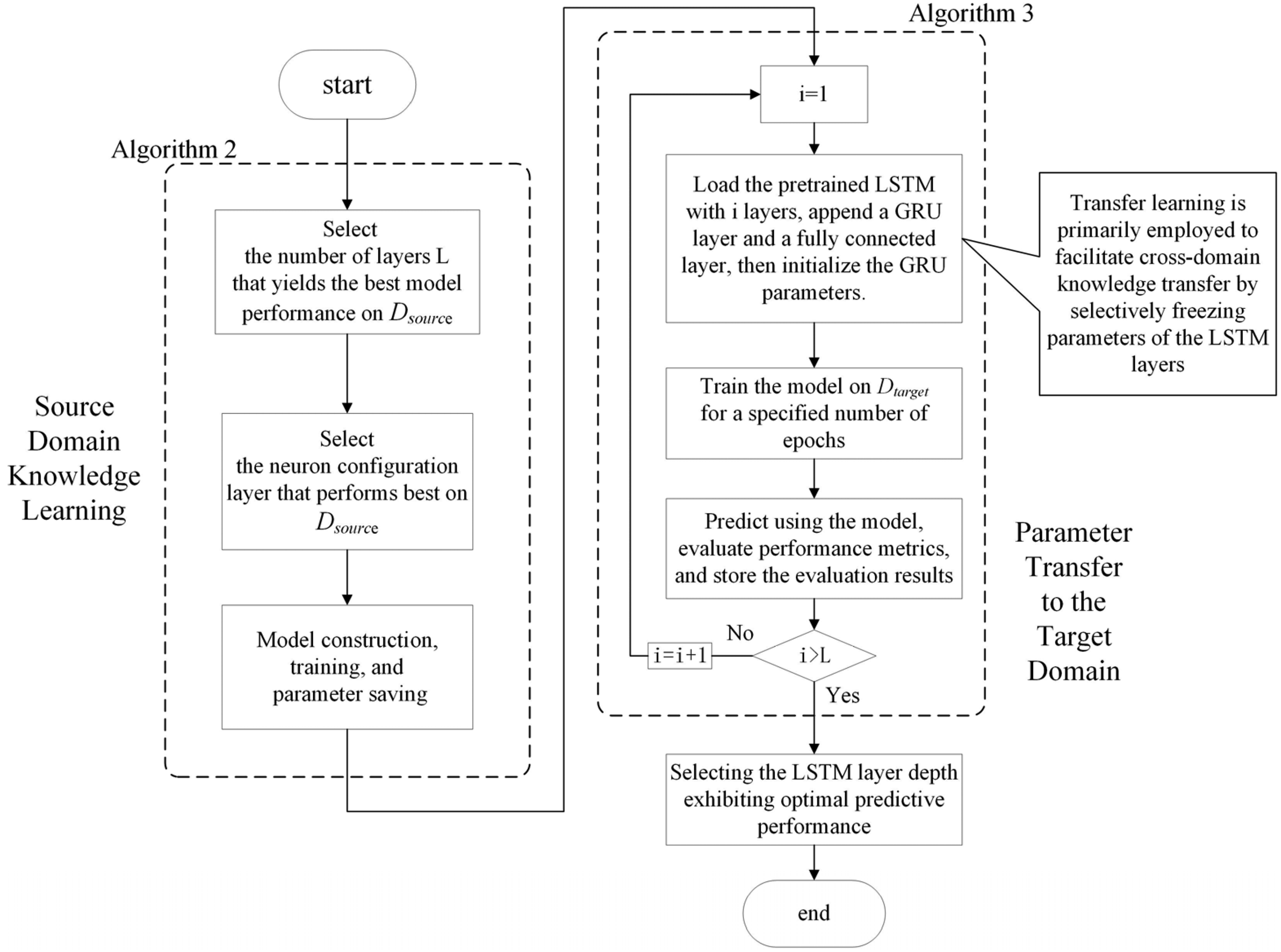

When transferring to the target domain, Algorithm 3 is employed: the input data are transformed through the frozen LSTM layer into the feature representation space learned from the source domain. This process enables the model to effectively inherit prior knowledge of temporal patterns from the source domain. On this basis, the trainable parameters of the subsequent GRU layer are dynamically adjusted to facilitate adaptive learning of temporal features specific to the target domain.

This hierarchical parameter optimization mechanism serves two purposes: on one hand, knowledge transfer through the LSTM layer alleviates insufficient feature learning caused by limited target domain samples; on the other hand, fine-tuning the GRU layer parameters enables the model to capture domain shift characteristics in the target domain. Together, these strategies contribute to building a temporal forecasting model with robust cross-domain generalization capability.

The use of parameter transfer strategies can effectively reduce the computational cost of the model. Without parameter transfer, the computational cost during backpropagation is as shown in equation (19). However, with transfer learning, the computation associated with the LSTM layer is omitted, resulting in a reduced cost as shown in equation (20).

{c o m p u t i o n}_{s i n g l e_d o m a i n} = O (T \cdot (N_{L S T M} + N_{G R U}))

(19)

{c o m p u t i o n}_{t r a n s f e r} = O (T \cdot N_{G R U})

(20)

In the above equation, T denotes the batch size during training, and N represents the number of trainable parameters in the current model.

Dual-phase transfer framework for wind power forecasting

As illustrated in Figure 8, this study designs a dual-phase transfer mechanism comprising two core stages: pretraining and transfer learning.

Figure 8.

Dual-phase transfer framework.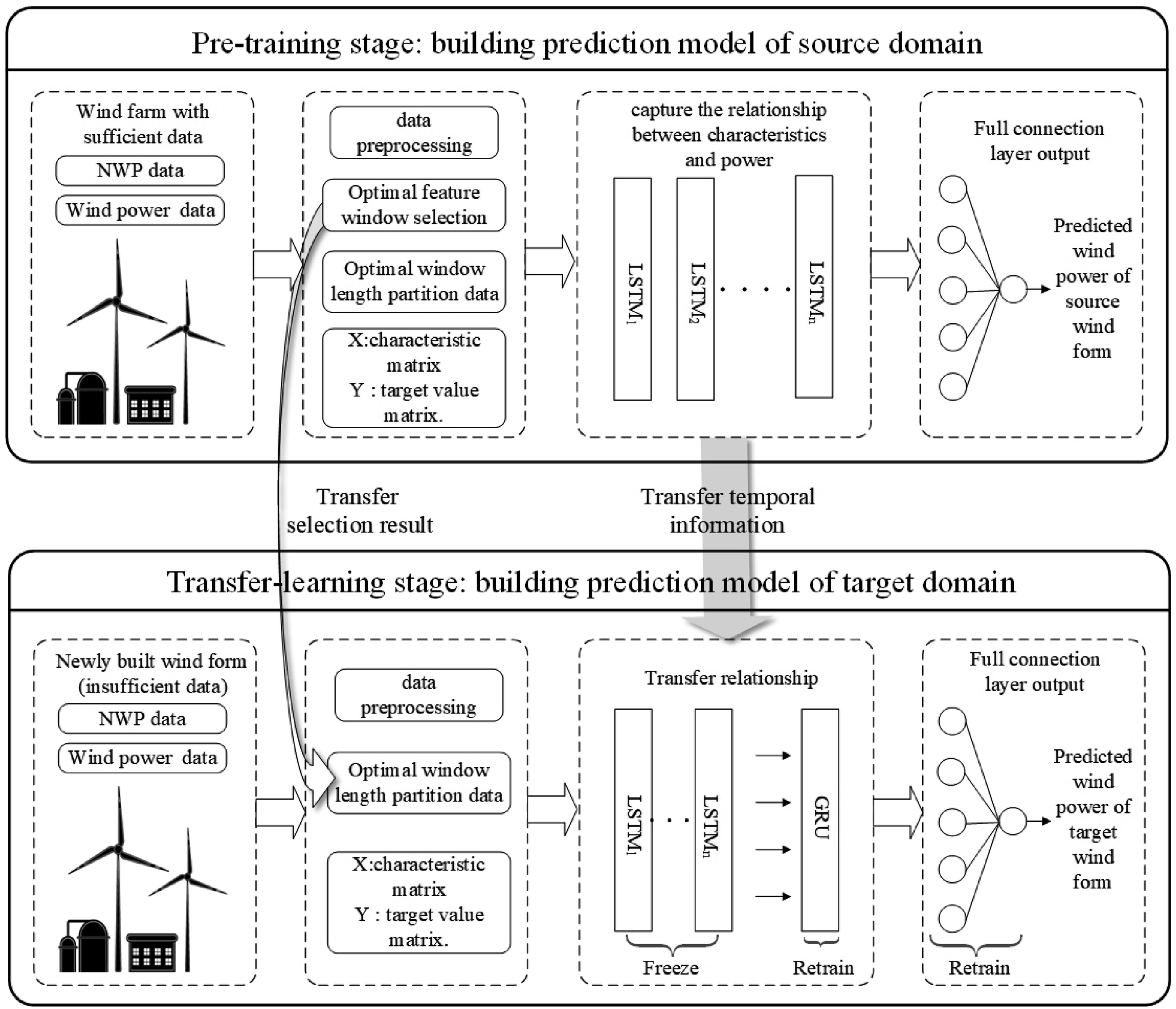

In the pretraining phase, based on the source-domain wind farm dataset with complete historical data, the optimal feature window is selected to construct feature matrices, while the layer depth and neuron count of the LSTM network are optimized to fully extract nonlinear mappings between temporal features and power output.

During the transfer learning phase, the source-domain optimal feature window is applied to partition target-domain (new wind farm) data. Partial hidden-layer parameters of the source-domain LSTM network are transferred as the feature extraction backbone, with tunable GRU layers introduced to adaptively model target-domain dynamic feature distributions.

By freezing transferred LSTM parameters to stably inherit cross-domain knowledge and dynamically optimizing target-domain feature representations through GRU layer parameter tuning, a hybrid architecture is ultimately constructed that integrates domain-invariant pattern learning with target-specific characteristic mining.

Experiments

To validate the effectiveness of the proposed model, this section presents a series of concrete experiments and detailed evaluations based on empirical data.

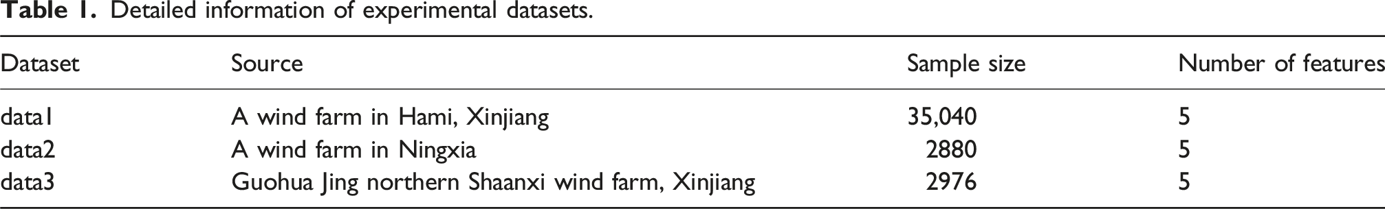
Experimental dataset

The wind power forecasting experiments in this study were conducted using the Python programming language, implemented with the TensorFlow deep learning framework (version 2.9.0). The Python version used was 3.8.10. All experiments were performed on a system equipped with a GeForce RTX 3090 GPU with 24 GB of memory.

The source domain dataset, data1, used in the experiments was collected from a wind farm located in Hami, Xinjiang, China. The target domain datasets, data2 and data3, were obtained from wind farms in Ningxia and northern Shaanxi operated by Guohua Energy. The datasets include real-time monitoring indicators closely related to wind turbine operation, such as wind speed, wind direction, temperature, and atmospheric pressure.

The basic information of the selected datasets is summarized in the Table 1 and Table 2. Table 1 provides basic statistical information including the collection location, sample size, and number of features for each dataset. Table 2 presents the value ranges of each feature in the form of closed intervals [minimum, maximum]. Among them, data1 encompasses the annual variation range of meteorological characteristics in the source domain, while data2 and data3 represent the variation ranges of meteorological features over 1 month in the target domains.

Table 1.

Detailed information of experimental datasets.

Dataset	Source	Sample size	Number of features
data1	A wind farm in Hami, Xinjiang	35,040	5
data2	A wind farm in Ningxia	2880	5
data3	Guohua Jing northern Shaanxi wind farm, Xinjiang	2976	5

Table 2.

Value ranges of key features in source and target datasets.

	Wind speed (m/s)	Wind direction (°)	Temperature (°C)	Atmospheric pressure (hPa)	Humidity (%)
data1	[0.0,23.963]	[0.0,359.884]	[−18.662,40.131]	[874.584,905.307]	[2.506,94.921]
data2	[0.4,16.5]	[0.0,356.9]	[−16.72,6.17]	[822.9,840.0]	[15.88,99.0]
data3	[0.32,19.783]	[0.0,355.607]	[12.822,15.331]	[861.012,882.02]	[28.426,95.273]

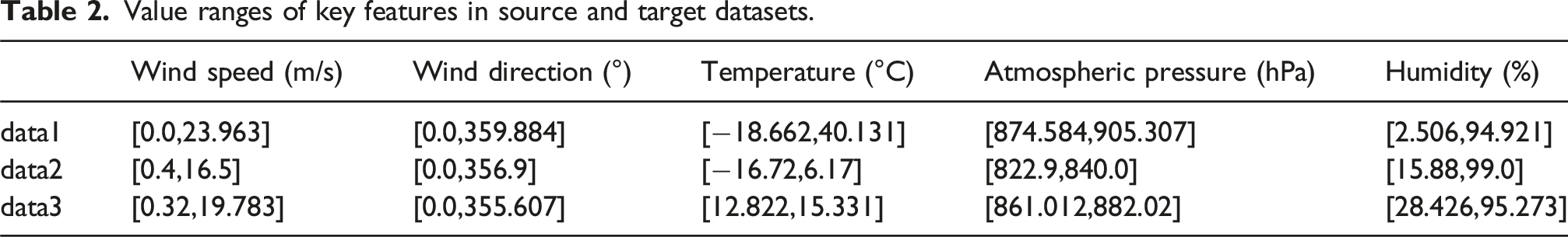
The geographic similarity in climate conditions between the source and target wind farm locations, along with the inclusion of all critical feature types and their corresponding value ranges from the target datasets within the source dataset, establishes favorable conditions for effective knowledge transfer through transfer learning.

The dataset is divided into training, validation, and test sets in a 7:1:2 ratio to perform 15-min-ahead wind power forecasting. To ensure training stability and accelerate convergence, Z-score standardization was applied to preprocess the data, transforming it into a distribution with a mean of 0 and a standard deviation of 1.

x_{n o r m} = \frac{x - μ}{σ}

(21)

Here, x represents the original (unprocessed) value, $x_{n o r m}$ denotes the normalized value, μ is the mean of the feature, and σ is the standard deviation.

Consequently, the model’s outputs are forecasts on the standardized scale. All performance metrics reported in the experiments were calculated based on this standardized scale to eliminate the influence of dimensional units and ensure a fair comparison. However, error metrics obtained from the standardized space lack immediate physical interpretability. Therefore, to enable a direct and intuitive comparison, both the model’s forecasts and the corresponding true values were inverse-transformed back to their original physical units (Megawatts, MW) prior to generating the performance curves.

Evaluation metrics

To assess the performance of the model in wind power forecasting, three different statistical metrics are employed: the R-squared Score (R²), Root Mean Squared Error (RMSE), and Mean Absolute Error (MAE).

R^{2} = 1 - \frac{\sum_{i = 1}^{n} {(y_{i} - ŷ_{i})}^{2}}{\sum_{i = 1}^{n} {(y_{i} - ȳ_{i})}^{2}}

(22)

RMSE = \sqrt{\frac{1}{n} \sum_{i = 1}^{n} {(y_{i} - ŷ_{i})}^{2}}

(23)

MAE = \frac{1}{n} \sum_{i = 1}^{n} | y_{i} - ŷ_{i} |

(24)

where

y_{i}

denotes the true value,

ŷ_{i}

represents the forecast value by the model, and

ȳ_{i}

is the mean of the true values.

Selection of the optimal temporal feature window length

The optimal length of the feature window is determined through experiments following Algorithm 1 outlined in the “optimal temporal feature window” section.

The model employs Mean Absolute Error (MAE) as the loss function and uses the Adam optimizer for training.

L = \frac{1}{n} \sum_{i = 1}^{n} | y_{p r e d, i} - y_{t u r e, i} |

(25)

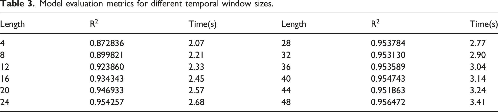
When the window length is set to 24, the R² score reaches 0.954,284. As shown in Figure 9, beyond this point, the R² values enter a plateau phase with only marginal gains (e.g., increasing the window size to 48 yields only an additional 0.23% improvement in R²). However, longer window length lead to a significant increase in training time—when the window length from 24 to 48, the time required per training epoch increases by 27%. Therefore, selecting a window length of 24 represents an optimal trade-off among forecasting accuracy, computational efficiency, and memory consumption (Table 3).

Figure 9.

Variation of R² with feature window length.

Table 3.

Model evaluation metrics for different temporal window sizes.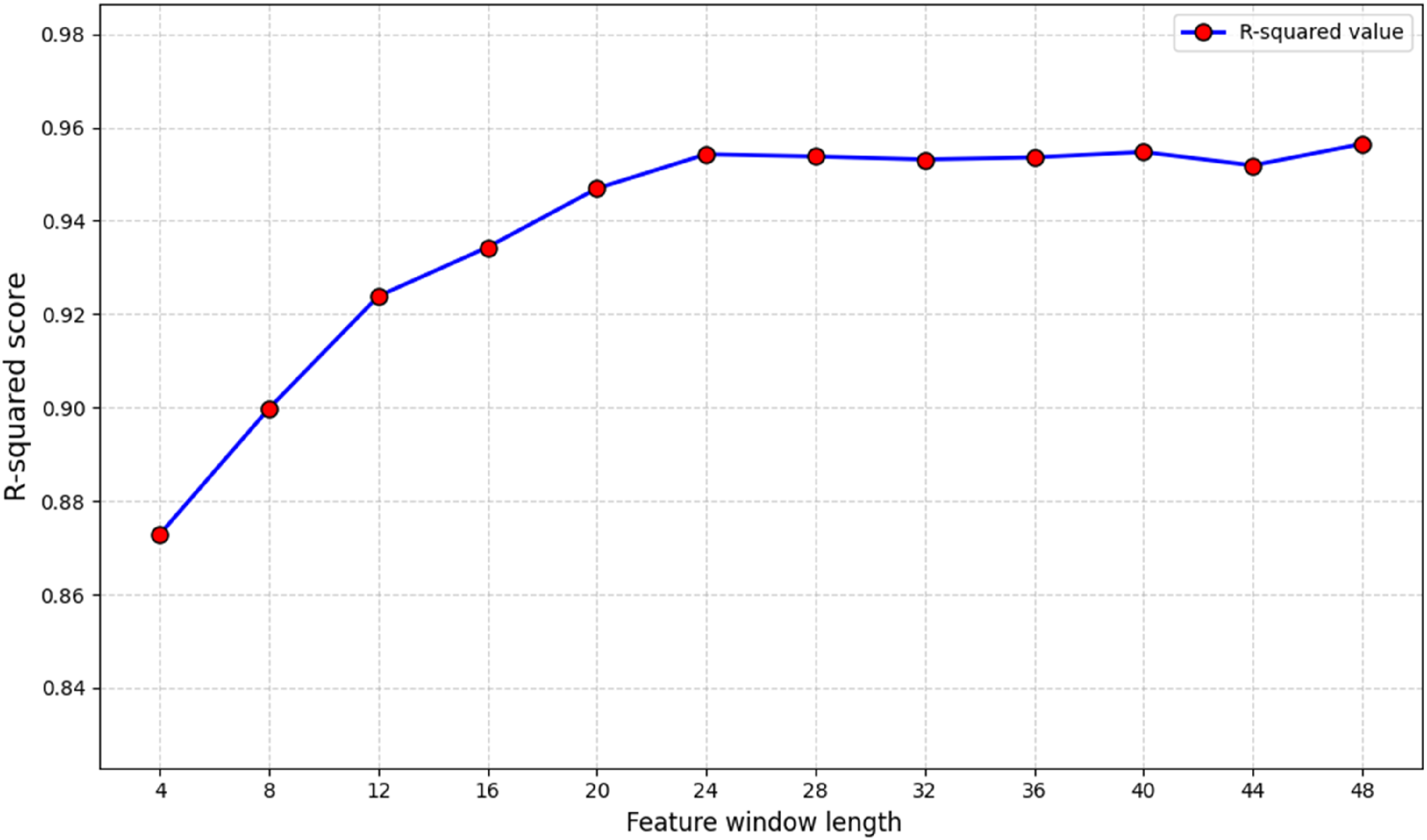

Length	$R^{2}$	Time(s)	Length	$R^{2}$	Time(s)
4	0.872836	2.07	28	0.953784	2.77
8	0.899821	2.21	32	0.953130	2.90
12	0.923860	2.33	36	0.953589	3.04
16	0.934343	2.45	40	0.954743	3.14
20	0.946933	2.57	44	0.951863	3.24
24	0.954257	2.68	48	0.956472	3.41

Source domain model construction

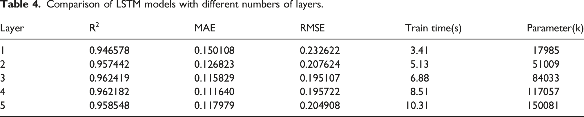
Based on Algorithm 2 in the “source domain model structure” section, the optimal combination of LSTM layer depth and neuron count is identified for the source domain dataset.

As shown in Table 4, when the number of LSTM layers reaches three or more, the model’s R² value stabilizes around 96%. Notably, with five LSTM layers, the R² score slightly decreases by 0.5%. In addition, increasing the number of layers leads to longer training time per epoch and a larger number of parameters. To avoid unnecessary computational and memory overhead, a three-layer LSTM architecture is selected as the optimal depth for the source model.

Table 4.

Comparison of LSTM models with different numbers of layers.

Layer	$R^{2}$	MAE	RMSE	Train time(s)	Parameter(k)
1	0.946578	0.150108	0.232622	3.41	17985
2	0.957442	0.126823	0.207624	5.13	51009
3	0.962419	0.115829	0.195107	6.88	84033
4	0.962182	0.111640	0.195722	8.51	117057
5	0.958548	0.117979	0.204908	10.31	150081

As illustrated in Table 5, different neuron configurations have a noticeable impact on the model MAE and RMSE values. When the neuron combination is set to 128–128–64, both MAE and RMSE reach their lowest values, indicating the highest forecasting accuracy on the source domain dataset.

Table 5.

Comparison of different neuron configurations.

	128–128–128	128–128–64	128–64–32	64–64–64	64–64–32
MAE	0.105151	0.089264	0.100025	0.115829	0.109482
RMSE	0.192060	0.168414	0.181842	0.195107	0.193004

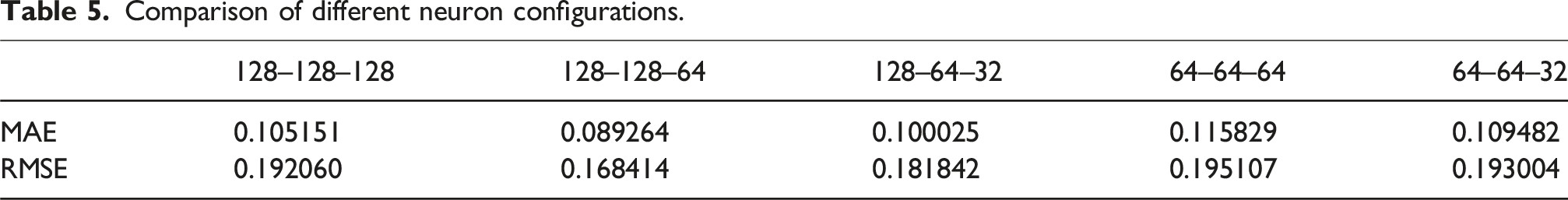
Figure 10(a) shows the scatter plot of forecast and true values. In this plot, the x-axis represents the true values, and the y-axis represents the forecast values. Most data points are concentrated near the dashed line (y = x), indicating a strong agreement between the forecasts and the true values. A small number of points exhibit noticeable deviations from the line, indicating occasional forecast errors; however, these deviations have a limited impact on the model’s overall performance.

Figure 10.

Forecasting results on the source domain dataset.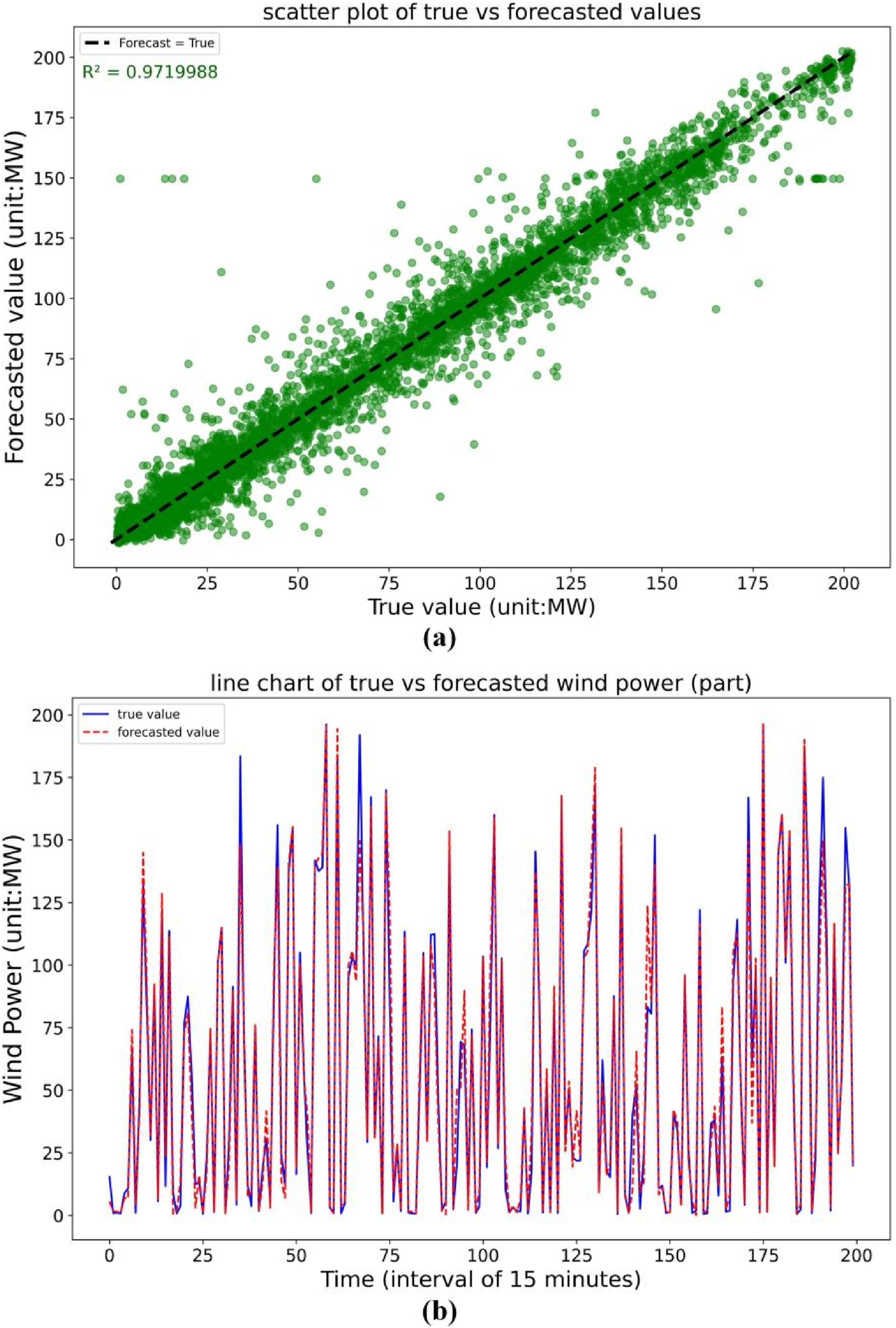

Figure 10(b) illustrates the temporal dynamics of the forecast and actual values. The forecast curve (dashed red) closely tracks the ground true (solid blue) overall. Although discrepancies exist at certain peaks—suggesting that the model’s peak forecasting capability could be improved—the overall close alignment demonstrates its effectiveness in capturing temporal patterns.

Determination of optimal frozen layer count for transfer model

Based on the pretraining process on the source dataset data1, a three-layer Long Short-Term Memory (LSTM) network model was constructed, which effectively captured the nonlinear dependencies between the multi-dimensional input features and power output through supervised learning.

Following Algorithm 3 (see the “frozen layer selection” section), this section investigates the impact of freezing different numbers of layers in this pre-trained model on the forecasting performance of the transferred model in the target domain.

As shown in Table 6, a frozen layer number of two yielded the lowest MAE and RMSE for the transfer model on both target domain datasets, indicating that the model exhibits the best fitting performance to the actual values under this configuration.

Table 6.

Impact of different numbers of frozen layers on the performance of the transfer model.

Layer	1		2		3
Layer	MAE	RMSE	MAE	RMSE	MAE	RMSE
data2	0.103202	0.151454	0.092371	0.1470025	0.164694	0.279249
data3	0.060401	0.112569	0.053620	0.103148	0.077057	0.135224

The scatter plots in Figure 11(a) and Figure 12(a)) show that most forecast values cluster near the diagonal (forecast = true line), indicating strong consistency with the true values, despite a small number of outliers. Similarly, the temporal dynamics in Figure 11(b) and Figure 12(b) confirm that the forecast values closely track the true values, further verifying the model’s effectiveness in learning relevant temporal features.

Figure 11.

Forecasting results on target dataset data2 with 2 frozen layers in the transfer model.

Figure 12.

Forecasting results on target dataset data3 with 2 frozen layers in the transfer model.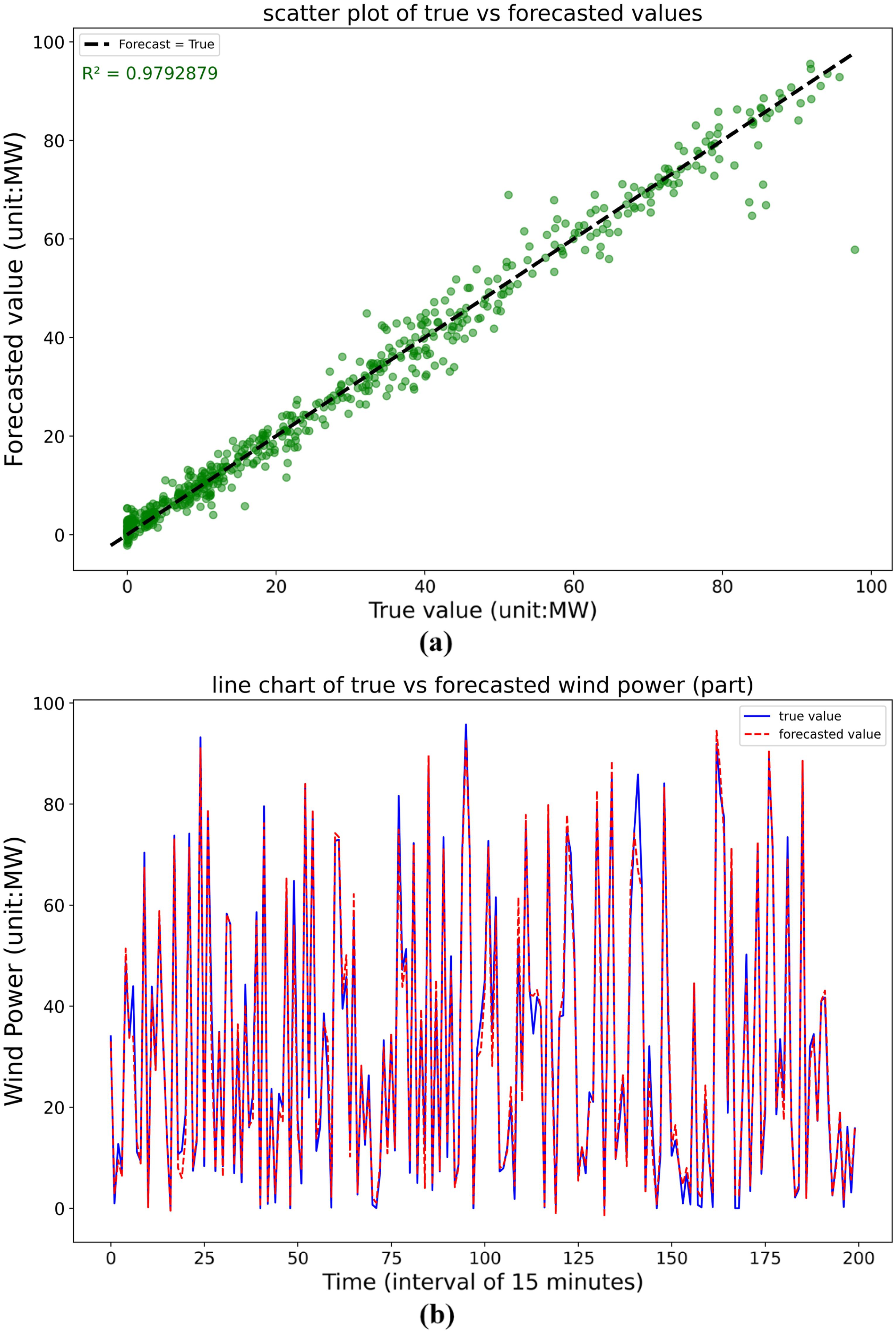

Transfer model configuration and robustness analysis

Based on the experimental results in the previous section, the model achieved optimal transfer performance on the target domain when the number of frozen layers was set to two. However, the training process of deep learning models often involves certain stochastic fluctuations, which may introduce deviations in the outcomes. To systematically evaluate the robustness of the model performance and the reproducibility of the results, this section details the hyperparameter configuration of the transfer model and presents multiple independent experimental validations.

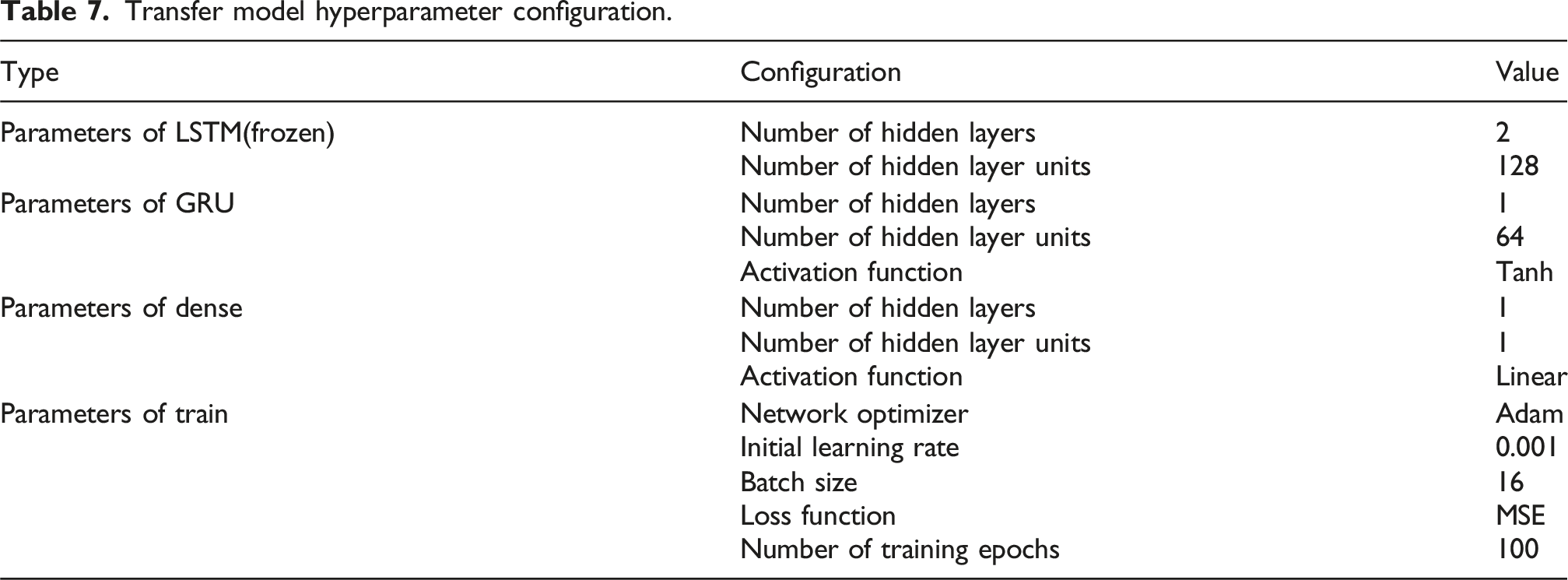
Table 7 comprehensively lists the hyperparameter configuration of the transfer model. To accurately assess the stability of the model performance and reproducibility of the results, five independent experimental runs were conducted on the proposed transfer model. The statistical results of these multiple experiments are presented in Table 8.

Table 7.

Transfer model hyperparameter configuration.

Type	Configuration	Value
Parameters of LSTM(frozen)	Number of hidden layers	2
Parameters of LSTM(frozen)	Number of hidden layer units	128
Parameters of GRU	Number of hidden layers	1
	Number of hidden layer units	64
	Activation function	Tanh
Parameters of dense	Number of hidden layers	1
	Number of hidden layer units	1
	Activation function	Linear
Parameters of train	Network optimizer	Adam
	Initial learning rate	0.001
	Batch size	16
	Loss function	MSE
	Number of training epochs	100

Table 8.

Statistics of model performance based on five independent experiments.

		No.1	No.2	No.3	No.4	No.5	Mean ± std
data2	MAE	0.092371	0.097039	0.092095	0.090275	0.094815	0.093319 ± 0.002633
data2	RMSE	0.147002	0.149395	0.144298	0.141506	0.146743	0.145789 ± 0.002998
data3	MAE	0.053620	0.051697	0.056945	0.053359	0.055417	0.054208 ± 0.002020
data3	RMSE	0.103148	0.101836	0.104650	0.105730	0.107322	0.104537 ± 0.002146

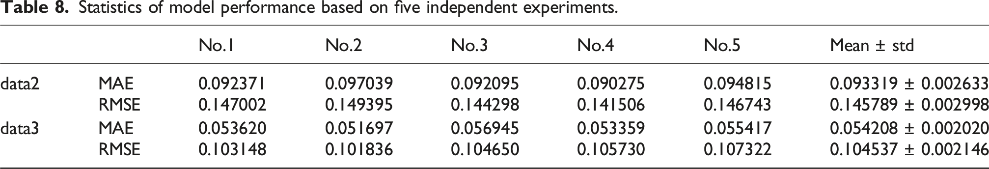
According to the results presented in Table 8, the proposed transfer learning model demonstrates high stability and reproducibility. On the target domain data2, the MAE and RMSE remain consistently at 0.093319 ± 0.002633 and 0.145789 ± 0.002998, respectively. Similarly, on the target domain data3, the values stabilize at 0.054208 ± 0.002020 for MAE and 0.104537 ± 0.002146 for RMSE. These results indicate that despite being trained multiple times, the model consistently converges to optima with similar performance, confirming the effectiveness and reliability of the proposed transfer strategy for both target domains, data2 and data3.

Comparative analysis of transfer model and other models

This section conducts experimental analysis on the efficacy of the transfer model for wind power forecasting.

For the purpose of model performance comparison, this section utilizes the results from the experiments presented in the “transfer model configuration and robustness analysis” section. An aggregate metric was constructed by summing the MAE and RMSE values for each experimental run. The median of this aggregate metric (corresponding to Run No. 1 for data2 and Run No. 4 for data3) was selected for comparative analysis, thus guaranteeing the representativeness and impartiality of the comparison.

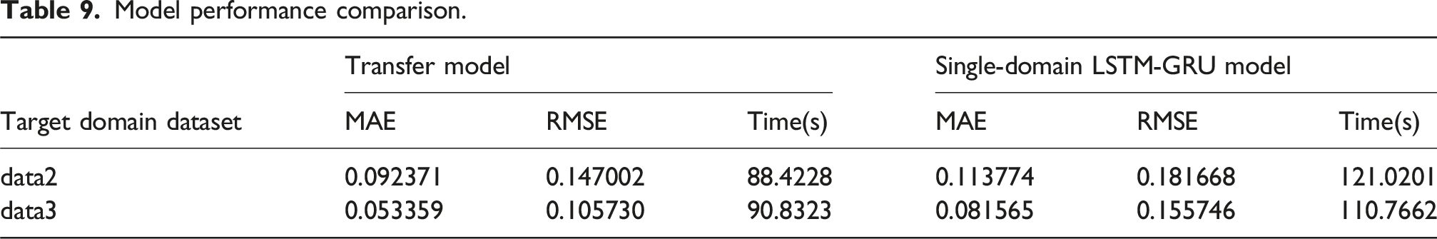
Transfer versus single-domain LSTM-GRU model

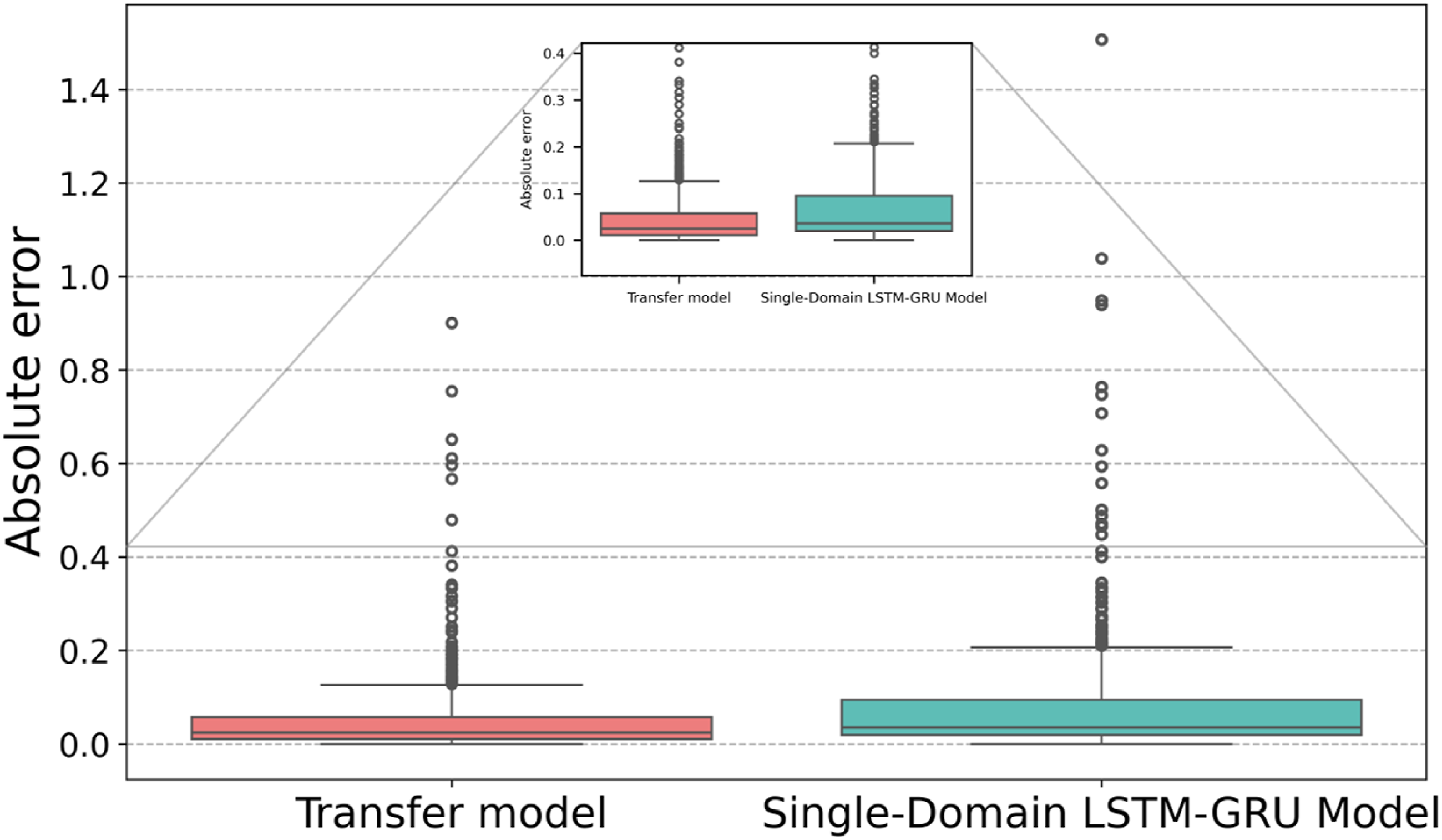
To validate the efficacy of source-domain parameters in the transfer model, a structurally identical single-domain LSTM-GRU model was constructed and exclusively trained on the target-domain dataset without external knowledge transfer. As shown in Table 9, the results demonstrate that on data 2, the transfer model achieved reductions of 18.8118% in MAE and 19.0817% in RMSE, while on data 3, it reduced MAE by 34.5810% and RMSE by 32.1138%. These improvements confirm the efficacy of transferring two pre-trained layers for enhancing wind power forecasting accuracy. Furthermore, by freezing transferred parameters during fine-tuning, the transfer model reduced training time by 32.5973 seconds (26.93544%) on data 2 and 19.9339 seconds (17.9964%) on data 3 (Figures 13 and 14).

Figure 13.

Distribution of forecasting errors on the target dataset data2.

Figure 14.

Distribution of forecasting errors on the target dataset data3.

Figure 15.

Comparison of forecasting results of different models on target domain data2.

Figure 16.

Comparison of forecasting results of different models on target domain data3.

Comparative analysis of the forecasting performance of the transfer model

To verify the performance advantages of the proposed model, this section conducts comparative experiments by evaluating the transfer model against classical machine learning models such as SVM and mainstream deep learning models including RNN and CNN, using the same target domain datasets.

Table 9.

Model performance comparison.

Target domain dataset	Transfer model			Single-domain LSTM-GRU model
Target domain dataset	MAE	RMSE	Time(s)	MAE	RMSE	Time(s)
data2	0.092371	0.147002	88.4228	0.113774	0.181668	121.0201
data3	0.053359	0.105730	90.8323	0.081565	0.155746	110.7662

Table 10.

Comparison of model performance on the target domain.

		SVM	RNN	CNN	TCN	Transfer model
data2	MAE	0.278348	0.253645	0.194429	0.156576	0.092371
data2	RMSE	0.438102	0.362148	0.266050	0.219676	0.147002
data3	MAE	0.137586	0.184137	0.121023	0.108770	0.053359
data3	RMSE	0.237314	0.333095	0.190699	0.158674	0.105730

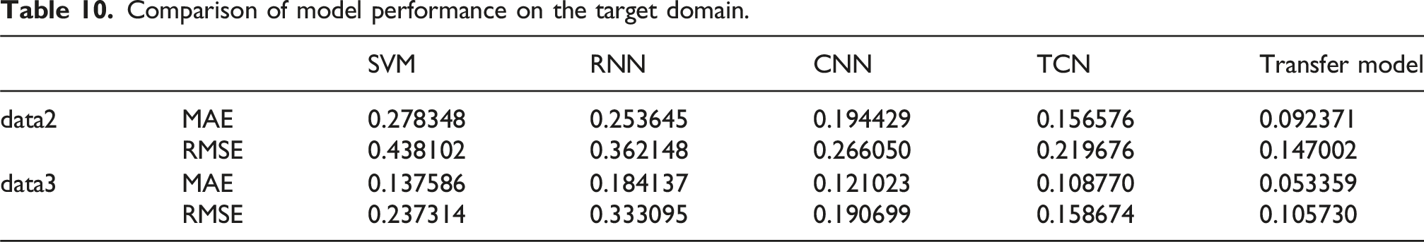
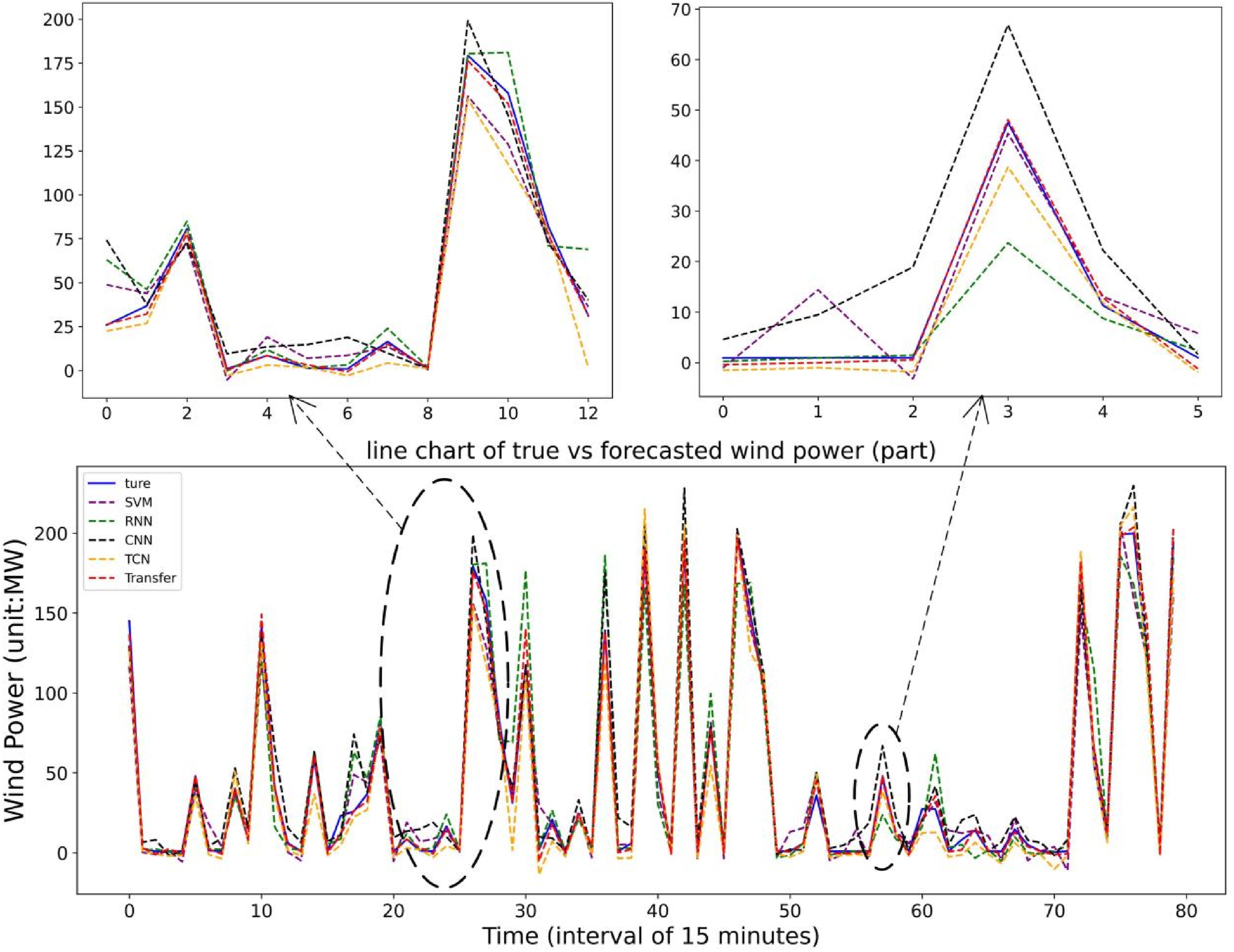
As shown in Figures 15 and 16, the forecast curve of the transfer model exhibits the closest agreement with the true values compared to the other models. The error metrics in Table 10, Figure 17, and Figure 18, the proposed transfer learning-based LSTM-GRU wind power forecasting model demonstrates substantial improvements over SVM, RNN, CNN, and TCN architectures. On target dataset data2, the proposed model achieves an MAE of 0.092371 – representing reductions of 66.8145% versus SVM, 63.5825% versus RNN, 52.4911% versus CNN, and 41.0056% versus TCN. Similarly, on data3, it attains an MAE of 0.053,359 with error reductions of 61.2177% against SVM, 71.0221% against RNN, 55.9100% against CNN, and 50.9433% against TCN.

Figure 17.

Comparison of forecasting errors of different models on target domain data2.

Figure 18.

Comparison of forecasting errors of different models on target domain data3.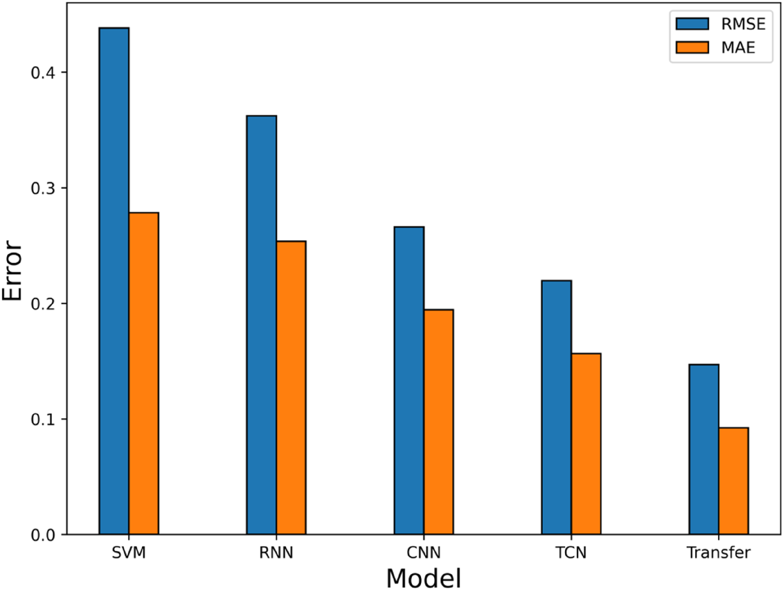

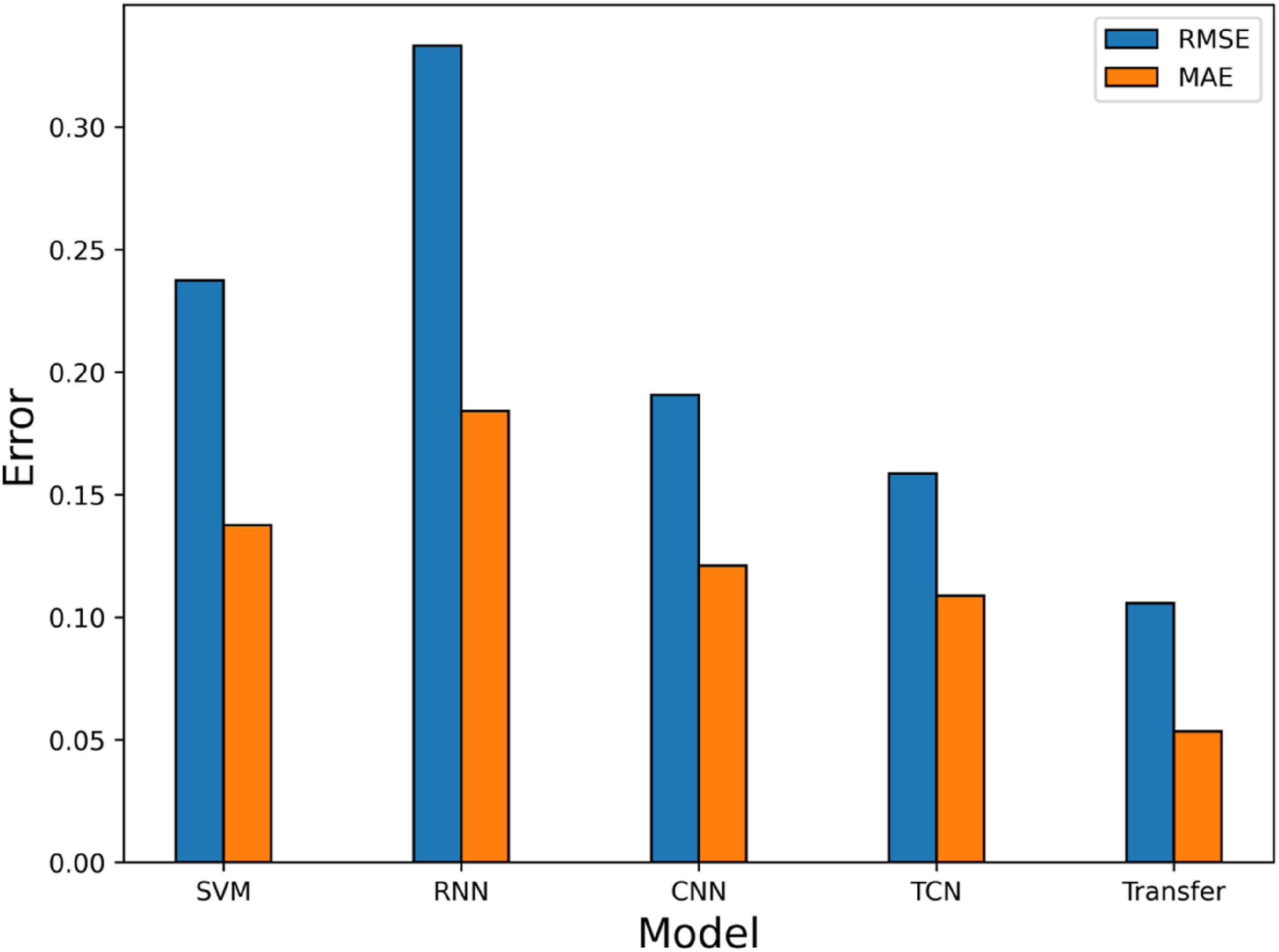
This improvement is primarily attributed to the fact that, under limited data conditions in the target domain, part of the model parameters are inherited from a pre-trained model on a larger-scale source domain dataset. These pre-trained parameters effectively capture complex nonlinear relationships between input features and the target variable, thereby enhancing the model’s generalization capability and forecasting accuracy on small-sample target domain datasets.

In summary, the transfer learning-based LSTM-GRU model demonstrates strong adaptability in wind power forecasting tasks involving small-scale datasets. By incorporating pre-trained parameters from the source domain, the model effectively captures the nonlinear relationships between temporal features and power output, even under limited target domain samples. This approach mitigates underfitting caused by scarce training data, significantly enhancing forecasting performance.

Conclusion

This study proposes a transfer learning-based LSTM-GRU model for wind power forecasting, specifically designed for newly constructed wind farms with scarce historical operational data. The model employs LSTM as its foundational architecture, pre-trained on data-rich source domain. During pre-training, the LSTM source model learns the complex nonlinear mappings between input features and power output, building a robust knowledge foundation for transfer. In the transfer phase, the model enables dynamic adaptation to target datasets through GRU parameter optimization for optimal forecasting performance.

Furthermore, the selection of an optimal feature window length for constructing the input matrices helps preserve essential temporal dynamics while minimizing noise interference. Experimental results demonstrate the model’s efficacy. Compared to a structurally identical single-domain models without pre-training, the proposed transfer learning approach significantly reduces MAE and RMSE on both target datasets (data2 and data3). It also shortens training time and improves computational efficiency. Benchmarking against SVM, RNN, CNN, and TCN models further confirms its superior forecasting accuracy, evidencing the efficacy of this transfer learning approach for data-scarce wind farms.

While the theoretical framework and empirical validation form the core of the research, the findings also carry significant managerial implications by providing a structured basis for rapid commissioning and stable operation of new wind farms, improving grid dispatch efficiency, and enhancing the reliability of investment decision-making.

Future work will focus on training source models with larger datasets containing richer features to expand scenario coverage and forecasting accuracy, conducting cross-dataset transfer experiments to enhance generalization capabilities, and exploring architectural innovations (e.g., attention mechanisms and meta-learning) to boost accuracy and domain adaptation for heterogeneously distributed datasets.

Footnotes

ORCID iDs

Weijing Nie

Ning Li

Author contributions

Zhengqiang Yang: Supervision and conceptualization. Weijing Nie: Methodology and writing—original draft. Weize Xu: Investigation and validation. Xin Zhang: Data curation and software. Ning Li: Funding acquisition and supervision

Funding

The authors disclosed receipt of the following financial support for the research, authorship, and/or publication of this article: This work was supported by the Natural Science Basic Research Program of Shaanxi Province (2025JC-YBMS-795).

Declaration of conflicting interests

The authors declared no potential conflicts of interest with respect to the research, authorship, and/or publication of this article.

Data Availability Statement

The data that support the findings of this study are available from the corresponding author upon reasonable request.*

References

Azimi

Ghofrani

Ghayekhloo

(2016) A hybrid wind power forecasting model based on data mining and wavelets analysis. Energy Conversion and Management 127: 208–225.

D-PN

Lee

Choi

(2016) Hourly average wind speed simulation and forecast based on ARMA model in Jeju Island, Korea. Journal of Electrical Engineering and Technology 11(6): 1548–1555.

El-Fouly

THM

El-Saadany

Salama

MMA

, et al. (2006) Grey predictor for wind energy conversion systems output power prediction. IEEE Transactions on Power Systems 21(3): 1450–1452.

Xiang

Zhang

, et al. (2021) Hybrid forecasting method for wind power integrating spatial correlation and corrected numerical weather prediction. Applied Energy 293: 116951.

Yao

, et al. (2025) Ultra-short-term prediction for wind power via intelligent reductional reconfiguration of wind conditions and upgraded stepwise modelling with embedded feature engineering. Renewable Energy 240: 122155.

Jalali

SMJ

Ahmadian

Khodayar

, et al. (2022) An advanced short-term wind power forecasting framework based on the optimized deep neural network models. International Journal of Electrical Power & Energy Systems 141: 108143.

Khalid

Savkin

(2012) A method for short-term wind power prediction with multiple observation points. IEEE Transactions on Power Systems 27(2): 579–586.

Lahouar

Ben Hadj Slama

(2017) Hour-ahead wind power forecast based on random forests. Renewable Energy 109: 529–541.

Luo

Liu

, et al. (2022) Wind power prediction based on EEMD-Tent-SSA-LS-SVM. Energy Reports 8: 3234–3243.

10.

Liao

Cao

Chen

, et al. (2023) Probabilistic wind power forecasting for newly-built wind farms based on multi-task gaussian process method. Renewable Energy 217: 119054.

11.

Liu

Zhou

Qian

(2021) Short-term wind power forecasting by stacked recurrent neural networks with parametric sine activation function. Electric Power Systems Research 192: 107011.

12.

Liu

Zhao

, et al. (2024) A bayesian deep learning-based adaptive wind farm power prediction method within the entire life cycle. IEEE Transactions on Sustainable Energy 15(4): 2663–2674.

13.

Behbood

Hao

, et al. (2015) Transfer learning using computational intelligence: a survey. Knowledge-Based Systems 80: 14–23.

14.

Lydia

Suresh Kumar

Immanuel Selvakumar

, et al. (2016) Linear and non-linear autoregressive models for short-term wind speed forecasting. Energy Conversion and Management 112: 115–124.

15.

Mei

Wang

Luo

, et al. (2024) Short-term wind power prediction based on encoder–decoder network and multi-point focused linear attention mechanism. Sensors 24(17): 5501.

16.

Meng

Chen

, et al. (2022) A novel few-shot learning approach for wind power prediction applying secondary evolutionary generative adversarial network. Energy 261: 125276.

17.

Nguyen

HKM

Phan

Q-D

Y-K

, et al. (2023) Multi-step wind power forecasting with stacked temporal convolutional network (S-TCN). Energies 16(9): 3792.

18.

Riedel

Belkilani

Reichert

, et al. (2024) Enhancing PV feed-in power forecasting through federated learning with differential privacy using LSTM and GRU. Energy and AI 18: 100452.

19.

Wang

AlShelahi

You

, et al. (2021) Integrative density forecast and uncertainty quantification of wind power generation. IEEE Transactions on Sustainable Energy 12(4): 1864–1875.

20.

Wang

Yang

Zhang

(2023) Wind power group prediction model based on multi-task learning. Electronics 12(17): 3683.

21.

Wang

Zhao

Hao

, et al. (2024) Short-term wind power prediction using a novel model based on butterfly optimization algorithm-variational mode decomposition-long short-term memory. Applied Energy 366: 123313.

22.

Xiu

Guo

(2013) Wind speed prediction by chaotic operator network based on kalman filter. Science China Technological Sciences 56(5): 1169–1176.

23.

Yang

Guo

Huang

, et al. (2025) Power prediction considering NWP wind speed error tolerability: a strategy to improve the accuracy of short-term wind power prediction under wind speed offset scenarios. Applied Energy 377: 124720.

24.

Yin

Chen

, et al. (2025) Few-shot wind power prediction using sample transfer and imbalanced evolved neural network. Energy 328: 136375.

25.

Zhao

Yun

Jia

, et al. (2023) Hybrid VMD-CNN-GRU-based model for short-term forecasting of wind power considering spatio-temporal features. Engineering Applications of Artificial Intelligence 121: 105982.

26.

Zhao

Gao

, et al. (2024) CPTCFS: CausalPatchTST incorporated causal feature selection model for short-term wind power forecasting of newly built wind farms. International Journal of Electrical Power & Energy Systems 160: 110059.

27.

Zhao

Pan

Chen

, et al. (2025) Intraday wind power forecasting by ensemble of overlapping historical numerical weather predictions. IEEE Transactions on Sustainable Energy 16(2): 1315–1328.