
Abstract
We explore the impact of delisting on the performance of the momentum trading strategy in Australia. We employ a new dataset of hand-collected delisting returns for all Australian stocks and provide the first study outside the U.S. to jointly examine the effects of delisting and missing returns on the magnitude of momentum profits. In the sample of all stocks, we find that the profitability of momentum strategies depends crucially on the returns of delisted stocks, especially on bankrupt firms. In the sample of large stocks, however, the momentum effect remains strong after controlling for the effect of delisted stocks, in contrast to the U.S. evidence in which delisting returns can explain 40% of momentum profits. As these large stocks are less exposed to liquidity risks, the momentum effect in Australia is even more puzzling than in the U.S.
1. Introduction
One of the most persistent challenges to the efficient market hypothesis is the trading strategy of momentum. Momentum investing strategies exploit historical trends in stock prices by buying winner stocks, those stocks that earned the best returns over some short time horizon (typically the past 3–12 months), and simultaneously short selling losers, those stocks that earned the worst returns over the same period. Jegadeesh and Titman (1993) were among the first to show that the momentum portfolios produce significant abnormal profits, generating 1.3% per month in the U.S. between 1965 and 1989.
The momentum effect does not appear to be sample-specific. Grundy and Martin (2001) demonstrated that momentum strategies have been profitable since the 1920s in the U.S., and have not vanished as some other anomalies appear to have. Also, it is not restricted to the U.S. market. Rouwenhorst (1998), Griffin et al. (2003) and Chui et al. (2010) document the profitability of momentum strategies in international equity markets. As Jegadeesh and Titman (2001) showed, the momentum effect does not appear to be due to data-snooping biases, as defined by Lo and MacKinlay (1990a). In a recent literature survey, Jegadeesh and Titman (2011) confirmed that the momentum strategy is still profitable, earning an average return of about 1.13% per month between 1990 and 2009.
Although data-snooping bias does not seem to explain momentum’s profitability, data problems, such as the omission of delisting returns, can still play an important role. The impact of omitting delisting returns (and, hence, delisted stocks) on asset pricing anomalies has been well documented in the U.S. Shumway (1997) was the first to point out the problem of missing delisting returns in the most common financial database, CRSP (Center for Research in Security Prices), and this problem is particularly severe for firms with poor performance. 1 Consequently, Shumway (1997, p. 340) points out that “in view of the delisting bias, researchers should be explicit about how they handle delisting returns”. Shumway and Warther (1999) further confirmed this problem and examined its impact on the size effect. They find that when delisting returns are included, especially for Nasdaq stocks, the size effect disappears.
More recently, Beaver et al. (2007) pointed out that delisting returns are not properly calculated in the monthly CRSP dataset and a large number of delisting returns are missing even after CRSP corrected the problems of Shumway (1997). They showed that correctly computing delisting returns and matching with Compustat’s accounting data has a large impact (of varying direction) on accounting-based anomalies. In the momentum literature, Eisdorfer (2008) found that approximately 40% of momentum returns in the U.S. are attributable to delisting returns and momentum is stronger in the group of delisted stocks. 2
Overall, the U.S. evidence suggests that correctly accounting for delisting returns is important and can have an impact on the magnitude of asset pricing anomalies, especially momentum. However, there has been virtually no research on the impact of delisting returns in markets outside the U.S. 3 Using a new dataset of hand-collected delisting returns for the Australian market, we fill this gap by providing the first out-of-sample evidence of the impact of delisting returns on the momentum anomaly.
The Australian market is an interesting case to consider because the Australian Securities Exchange (ASX) is relatively large, being the eighth largest equity market in the world (based on free-float market capitalization) and the second largest in the Asia-Pacific area, with A$1.2 trillion market capitalization, 4 and especially it uses a different trading mechanism. The different trading mechanism leads to another vexing issue, which is the problem of missing trades caused by illiquidity among smaller stocks. This is an important problem when dealing with the Australian stock market for two reasons. First, the Australian market simply has less turnover than the larger U.S. markets, and this is especially true among stocks that are not in the main index (Comerton-Forde et al., 2010). Second, the ASX uses automatic trade execution via a limit order book, which is in contrast to the New York Stock Exchange’s use of specialists that post bid and ask prices with significant depth. The CRSP database uses the mid-point of the bid and ask prices to construct returns when a stock has zero trading activity in any given month, but this practice seems less defensible in the Australian context of no specialist traders in a relatively illiquid market. We will explore the impact of missing returns, especially in the context of small illiquid stocks, using a range of different empirical methods.
Delisted stocks are crucially important for the profitability of momentum. There are two main reasons why a stock delists: being involved in a merger or bankruptcy (Eisdorfer, 2008). Both of these types of delisting tend to increase the momentum profitability. Acquired stocks often experience a price run-up prior to delisting, which is why they tend to be in the “winner” portfolio. If much of the momentum profits is due to merged stocks, then momentum would simply be another manifestation of the well-known behaviour of returns around mergers. On the other hand, since bankrupt stocks typically suffer a prolonged period of very poor performance prior to the actual bankruptcy and delisting, they tend to be in the “loser” portfolio. If momentum is due in large part to the poor performance of bankrupt stocks, then the strategy may not be investible since as a practical matter short selling such stocks is difficult, if not impossible, especially when the market is anticipating their impending doom.
We compare returns from the sample of delisted stocks and those stocks that survived to the end of our sample. When we focus the attention on the sample of delisted stocks, the average winner-minus-loser (WML) return is 1.86% (t-statistic = 4.88) per month. In the sample of surviving stocks, the momentum profit decreases to only 0.44% per month, which is statistically insignificant at even the 10% level. Thus, consistent with Eisdorfer (2008), the profitability of momentum strategies appears to be entirely due to the returns of delisted stocks. We also document that most of the delisting effect is directly attributable to the poor performance of bankrupt stocks.
There is a stark contrast between the liquidity of the largest stocks and smaller stocks. We undertake an analysis using the largest 300 stocks measured by market capitalization, denoted as the Top300. We find that delisting returns play a much less important role among the highly liquid Top300 stocks. Not only is the difference between average momentum profits with and without delisting returns economically insignificant, but the difference between the sample of only delisted stocks and surviving stocks reverses. The average momentum return in the sample of surviving stocks is 2.21% per month (t-statistic = 6.80) whereas that in the sample of only delisted stocks is only 0.46% per month (t-statistic = 1.23). This is because the average return to merged loser stocks is significant and positive, while the bankruptcy effect is dramatically reduced. Consequently, in the subsample of Top300, delisted stocks are not the explanation of momentum in Australia, inconsistent with the U.S. evidence of Eisdorfer (2008) in which 40% of momentum returns are attributable to the delisting effect. 5 This evidence also shows that momentum is even more puzzling in Australia because the Top300 stocks are more liquid and accessible to both institutional and individual investors.
Finally, this study is also motivated by the equivocal evidence of momentum in Australia. Hurn and Pavlov (2003), Demir et al. (2004) and Galariotis (2010) find significant average momentum profits of approximately 1.54% per month, while Durand et al. (2006b) and Brailsford and O‘Brien(2008) document no or weak momentum effects. It is interesting that the former studies restrict their focus to only the very largest Australian stocks, while the latter studies have a wider scope and include all stocks. 6 We conjecture that these different conclusions are driven by the presence or absence of smaller capitalization stocks and their delisting returns. 7
Interestingly, we indeed find that incorporating delisting returns in the calculation of momentum profits enhances the average momentum profit in the sample of all stocks from 0.68% per month (t = 2.22) to 0.76% per month with the t-statistic of 2.57, significant at the 1% level. The momentum effect is significantly stronger among the sample of largest stocks, earning a doubled average return of 1.49% per month (with delisting returns in place). This confirms our conjecture for the mixed Australian evidence, and provides a curious counterpoint to the U.S. evidence. The fact that the momentum effect is strongest among the most liquid stocks in Australia suggests that it would be easier to reliably implement such a trading strategy in Australia, 8 but also poses a more puzzling anomaly from an academic perspective as the returns to momentum cannot be compensation for bearing liquidity risk.
The remainder of the paper is structured as follows. We describe the data in Section 2. Section 3 outlines how we form portfolios and this is where we discuss our adjustments for delisting and non-trading on the data sources. We also discuss how we deal with missing returns. Section 4 reports the effect of delisting returns on momentum in the sample of all stocks as well as the top 300 stocks by market capitalization. We conclude in Section 5.
2. Data
Our data consists of monthly Australian equity returns between January 1993 and December 2008, obtained from the Center for Research in Finance (CRIF hereafter) database. This is the most comprehensive data available for Australian equities and has been used in comparable studies before. 9 The database includes monthly stock prices, dividends, adjustment for capitalization changes, returns and market capitalizations of all stocks listed on the ASX. Monthly returns are adjusted for changes to stock splits, dividends, spin-offs, rights issue and other capitalization changes. 10 The sample contains 3009 stocks. On average, there are around 1000 stocks per year available to construct the momentum trading strategies.
To construct the Fama and French’s (1993) high-minus-low (HML) (book-to-market (BM)) factor we require accounting data on the book value of total shareholder equity, which we obtain from MorningStar’s Aspect Huntley between June 1986 and December 2008. The constituent list of all stocks from Aspect is then used to match with the CRIF database to find the corresponding share prices. As is usual, we exclude firms with negative or missing book values. We follow the usual approach to compute the factors, which is outlined for convenience in the Appendix. A total of 2564 stocks remains in the sample. 11 The number of firms in our sample rises each year from 205 firms in 1986 to the peak of 1640 firms in 2008. The book-to-market ratio for each firm is then computed by dividing the lagged one-year book value (to ensure that the information is available to investors) by the price at the end of fiscal year (i.e. June).
3. Empirical methodology
3.1 Constructing momentum portfolios
Following the current literature, we construct the most common 6/1/6 momentum portfolios in which stocks are ranked based on their returns over the past 6 months, and then held for 6 months with 1 month skipped between the two periods. The skipping period, which is standard in the literature, avoids microstructure effects such as bid-ask bounce. 12 At the end of each month t, continuously compounded returns on each stock are computed as a criterion to rank stocks over the past 6 months (the ranking period). To be eligible for ranking, stocks must have a return history of 6 months and be actively traded from the beginning to the end of formation period. This restriction is imposed in an attempt to have a tradable strategy, since if a stock did not trade at the end of the ranking period the strategy would not have been investible. These requirements do not induce bias as all historical information is known prior to the portfolio formation time t.
Stocks are then grouped into quintiles where the top quintile consists of the best performers (winners) and the bottom quintile contains the worst performers (losers) during the ranking period. In the subsequent 6 months (the investment or holding period), the momentum strategy enters a long position in an equally weighted portfolio of winners and a short position in an equally weighted loser portfolio. Owing to this construction, momentum investing is also called a zero-cost or self-financing strategy. Momentum returns are then the equal-weighted average of all individual returns within the portfolios.
Consistent with international studies and Jegadeesh and Titman (1993), we only examine overlapping portfolios in which the strategy is followed every month. Similar to Brailsford and O‘Brien (2008) and Galariotis (2010), we form stocks into quintiles because the Australian market is small relative to the dominant U.S. markets, grouping stocks into deciles as in most U.S. studies will significantly reduce the number of stocks in winner and loser portfolios. This is a particularly vexing concern when we focus attention on the largest 300 stocks by market capitalization. As we employ overlapping returns, not overlapping data, usual t-statistic can be used without adjusting for serial correlation, assuming that there is no autocorrelation in monthly returns.
3.2 Survivorship biases
The Australian data has two complicating issues not present in, for example, the CRSP data used in U.S. studies. Firstly, CRIF does not record delisting returns, which is a problem also found in many other databases of non-U.S. returns. This creates severe complications for computing the returns to the momentum strategy, and can severely bias returns.
Although CRIF keeps records of the reasons for delisting (but not other detailed information such as off-exchange distributions), those reasons are not necessarily the principal causes as noted in the database guides. For example, a company that was acquired may stop paying listing fees to the ASX, and hence be recorded as “other reasons”, while it should belong to the category of “merger/acquisition”. As we will soon discuss, we overcome this problem by hand collecting the reason for delisting and off-exchange distributions using two other databases that track the company’s history for several years after delisting. Therefore, the reason for delisting that we record should be more accurate. The actual delisting return can vary widely: for example, it may be an off-exchange distribution to shareholders as a result of a merger or acquisition, which is typically a positive return; or a share cancelation, which typically generates large negative returns.
It is interesting to note that Grundy and Martin (2001) address this issue by deleting these stocks from their CRSP sample. In Australia, Demir et al. (2004) and Galariotis (2010) impose a similar restriction in their sample: requiring stocks to survive the first 2 days or 2 months of the holding period. This restriction may bias the size of momentum profits as it implicitly assumes that investors, who stand at the end of the ranking period and decide which stocks to pick/drop, possess “perfect foresight” of future delisting or acquisition activities and chose to omit those stocks from the portfolio in advance. 13
Accurately accounting for delisting returns is very important to measuring momentum’s profitability. Eisdorfer (2008) finds that approximately 40% of momentum returns are attributable to delisted stocks and that the momentum effect is stronger among bankrupt firms. However, Eisdorfer uses the original monthly delisting returns from CRSP in which, as Beaver et al. (2007), point out, many delisting returns are not properly calculated. Our dataset does not suffer from these problems as we manually compute final returns for each delisted stock.
The second problem with the CRIF database is missing returns caused by non-trading over possibly several months, making it impossible to compute returns over the non-trading interval. 14 In Australia, Hurn and Pavlov (2003) and Gray (2013) provide alternative methods to handle the bias. In dealing with delisted stocks, Hurn and Pavlov (2003) assume that those stocks are liquidated and subsequently worthless. This means that their prices are set to zeros and returns will be −100% in the delisting month and zeros in the subsequent months. Although this approach does not induce any perfect foresight, it severely depresses momentum returns, especially when stocks are delisted due to mergers or acquisitions in which investors may receive payments from acquirers. In this study, rather than treating all delisting returns the same, we employ a range of alternative replacement values for missing delisting returns, depending on the stock’s reason for delisting.
Hurn and Pavlov (2003) and Gray (2013) make a serious effort to handle missing returns. In the next section, we compare and contrast our methods of inferring missing values with theirs, and propose a new method that extends the regression-based approach of Hurn and Pavlov (2003). Finally, we will show that Hurn and Pavlov (2003) find similar results for different techniques because their examination is limited to the largest stocks. When small stocks are included, various approaches will produce differing results.
3.3 Delisted stocks
Of the 3009 stocks in our sample from January 1993 to December 2008, 969 stocks are delisted before the end of the sample period. Since there is no database that supplies delisting returns for the Australian market, we hand-collect delisting information and compute the corresponding returns from two sources. The first source is http://www.delisted.com.au, which contains delisting information of virtually all listed stocks. 15 We also use MorningStar’s DatAnalysis to cross check the information. The delisting information from both sources has to be hand-collected. We calculate delisting returns by extracting the text information (e.g. final dollar amount distributed to shareholders in the case of share cancelations or the final offer to target shareholders in the case of merger/acquisitions) and then comparing the value with the stock’s last trading price. As DatAnalysis’s coverage only started since the 1990s, we rely primarily on the first database for information prior to 1990.
We categorize delisted stocks into three main groups whose descriptive statistics are reported in panel A of Table 1. The first group consists of 655 stocks that are delisted due to mergers or acquisitions. Amongst them, 637 firms have sufficient details to compute the final delisting returns. Stocks in this group on average earn off-exchange returns of 0.51%, with the minimum and maximum delisting returns of −94% and −203.45%, respectively. The second group consists of 122 stocks that are not only delisted but also deregistered. We classify those stocks as bankruptcy only when the appointed liquidators confirmed to shareholders that no distributions would be made. Delisting returns on those stocks are thus −100%. The last category contains 192 stocks that go off the exchange because of share cancelations, failure to pay listing fees or other reasons but firms still survive. In this group, 141 delisting returns can be collected. The average delisting return of this group is −19.92% with minimum and maximum values of −100% and 116.10%, respectively.
Proportions of missing values and delisted stocks.
Panel A shows the whole-sample summary statistics on each category of delisting reasons namely merger related, bankruptcy and others between January 1993 and December 2008 (192 months). “N”, “T” and “STD” denote number of stocks, months and standard deviation, respectively. In panel A, the number in parentheses next to column “N” indicates the number of delisted stocks with delisting returns available from either http://www.delisted.com.au or MorningStar. The total number of delisted stocks over the sample period is 969 stocks. There are 3009 stocks over the entire sample. Panel B presents average percentages of missing values and delisted stocks in the composition of winner and loser portfolios. The momentum strategy considered here is 6/1/6, which ranks stocks over the past 6 months and then hold winner and loser stocks over the next 6 months, allowing 1 month skipping period in between. On average, momentum portfolios constructed from the sample of all stocks contain 290 stocks in each of the winner/loser portfolio a month, with a minimum and a maximum of 195 and 409 stocks, respectively. In the sample of Top300, the number of stocks in each winner/loser portfolio is maintained to be 60 stocks per month. In the filter, we require that stocks must have at least 24 valid returns over the past 60 months to be ranked. The proportions of missing values and delisted stocks are out of the total number of stocks in each winner/loser portfolio in a month. Panel B1 reports the percentage of missing returns during holding periods. Panel B2 reports the percentage of delisted stocks during holding periods. Percentages reported in parentheses are the corresponding delisting frequencies within the delisted winner/loser samples.
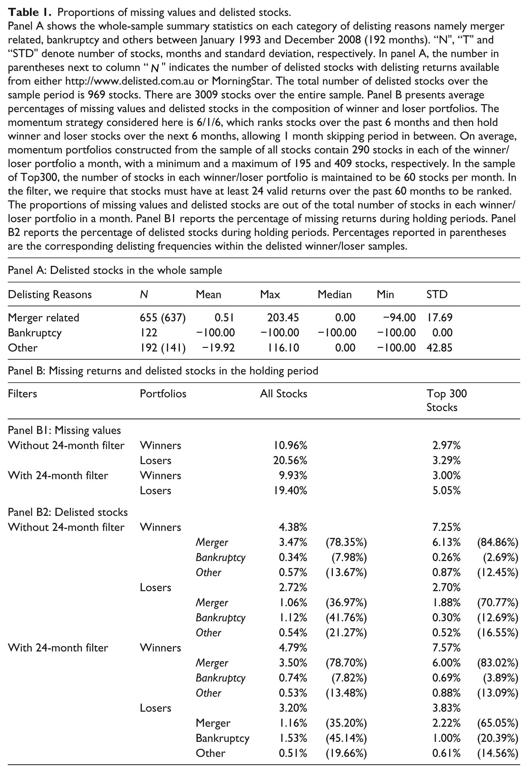
Delisting returns are calculated by comparing the value of the security after it is delisted from the exchange with its price on the last month of trading. The returns will then be included as the final month of trading in the holding period if the stock is delisted while being included in the momentum portfolios. For those stocks that we do not have sufficient information to compute delisting returns, we use its category’s average instead. These preliminary statistics indicate that the imposed −100% returns on all delisted stocks in Hurn and Pavlov (2003) do not represent the true return to shareholders and hence severely bias the finding of momentum.
3.4 Missing returns
The other main problem encountered with the CRIF database is the problem of missing returns that occur when stocks do not trade in every month. To illustrate, if a stock trades in December and then does not trade until February, then no return can be computed for January or February. To deal with the problem of missing returns we consider three alternative methods to compute returns on the momentum strategy: the CRIF approach, the sample mean, and a conditional expectation using a three-factor model.
The CRIF approach
If a stock does not trade in a month during the investment period, the last recorded price is used to compute returns. We term this method as the CRIF approach because it is used by CRIF to construct indices (see Hurn and Pavlov, 2003). This approach results in recording no trade in all months during which a stock does not trade, and the total return on the non-trading period is recorded in the single month in which the stock finally trades. Because we require a complete trading history over the ranking period for a stock to be ranked, this problem has been effectively assumed away. So assuming zero returns during all but the final month will tend to understate returns in the portfolio strategy. Gray (2013) also imposes the same trading price in the non-trading month as in the last valid month, but acknowledges that they are “ad hoc and clearly imperfect” (p. 9). This method also overstates the conditional variance of returns due to the fact that stale prices are followed by the new price, which contains new information that significantly changes the portfolio’s variance. This in turn will affect standard errors in formal hypothesis testing ex-post. Consequently, we propose a more calibrated “conditional expectation approach” as one of our three alternative methods. 16
The unconditional mean approach
In this approach, we replace missing returns during the holding period by the average of stocks’ historical returns. Although Hurn and Pavlov (2003) also employed this method, they replace missing returns with the sample mean before examining momentum portfolios. That way induces a look-ahead bias in portfolio selection. At the formation date t, if a stock does not trade, it cannot be bought or sold and hence should not be included in the portfolios. If the missing value is replaced in advance, it will become a valid trade and be falsely included in the momentum portfolios. 17
The conditional expectation approach
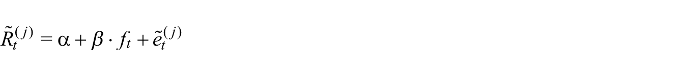
Under this method, returns are assumed to be generated by the factor model:
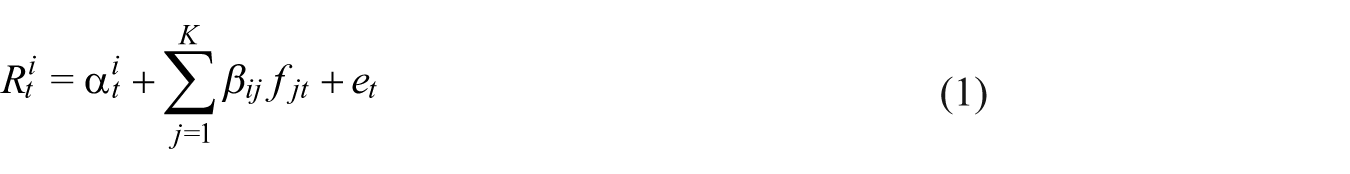
where
Our method extends the regression-based approach of Hurn and Pavlov (2003) who replace the missing return by its predicted value from a factor model using the market and industry returns. We construct the Fama and French factors and account for the actual return over the entire non-trading period. Unfortunately to account for the multiple-horizon discretely compounded return requires a simulation-based approach to compute the expectations.
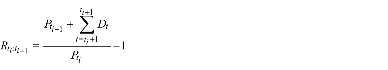
Denote by t i the date of the last time in each month that a stock records a valid trade, indexed by i indicating the month in which a valid price occurs. When t i +1−t i > 1 the stock is said to suffer from the non-trading problem, and we are unable to observe the return for any of the one-period returns between t i and t i +1. To compute the return on the momentum trading strategy, we replace each missing trading return with its expectation conditional on the sequence of one-period factor realizations and conditioning on the observed multi-period gross return between the two actual trade dates. Of course if the stock trades in sequential months, this is equal to the actual one-period return.
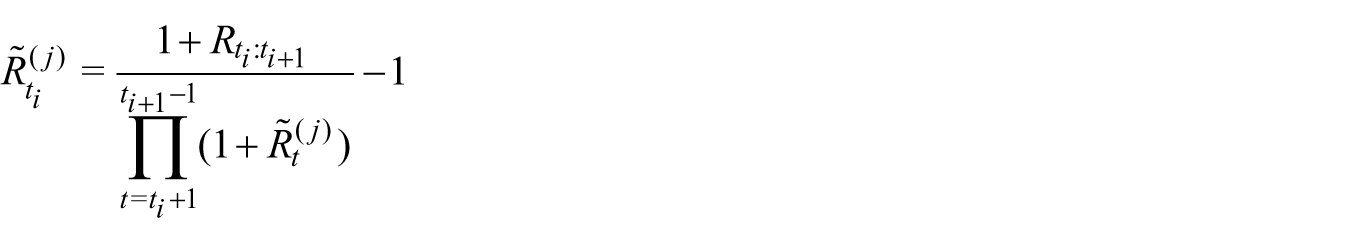
In particular, we replace missing returns for

where the total period return is given by
of course adjusting for dividends and capitalization changes. We propose a simple simulation scheme to compute these conditional expectations


using a simple simulation scheme that is inspired by the sampling-importance resampling scheme used in particle filtering. In particular, we simulate a total of N“particles”, which are simply collections of the one period returns
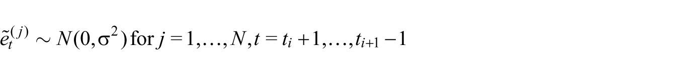
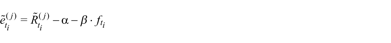
where σ2 is the residual variance for the stock under consideration. Note that we simulate up until the penultimate non-trading return period. The corresponding returns are given by
We are able to impose the constraint that the total discretely compounded return holds over the entire period by defining the final period return to equal
We then have
We are now in a position to compute the resampling weights imposing the constraint of all conditioning information using the conditional density:
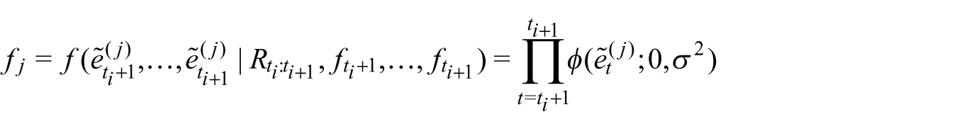
where

This effectively approximates the conditional random variables R with the discrete distribution located at

For the factor model we use the FF3F model and construct the size and value factor returns using hand-collected delisting return data. 18 To ensure our regression estimates are reliable we require that a stock must have at least 24 valid returns over the past 60 months to be included in winner and loser portfolios. This restriction does not induce any survivorship bias as the information is known by the time of portfolio formation.
3.5 Proportions of delisted firms and missing returns in the momentum portfolio
As mentioned in the previous subsection, delisted stocks account for approximately 32% of the whole sample. As momentum portfolios choose stocks in the two extreme quintiles, we are more interested in the proportions of delisted stocks and missing returns in winner and loser portfolios. Moreover, since the majority of stocks on the Australian market are small and illiquid, it is also reasonable to examine those proportions in the Top300 by market capitalization.
Table 1 reports the percentage of survivorship biases in winner and loser portfolios. We first look at the statistics of missing returns in panel A. In the sample of all stocks, on average 10.96% of the winners’ returns are missing while more than 20% of losers do not trade. This confirms our conjecture that loser stocks tend to be small and less liquid than winner stocks. If we limit the sample to the Top300 by market capitalization, loser portfolios still have more missing returns than winner counterparts although the proportions now significantly reduce to less than 4%. For the conditional expectation method of inferring missing returns, we also place a constraint that stocks must have at least 24 months of valid returns over the past 60 months in order to be included in the winner/loser portfolios. This filter nevertheless does not significantly reduce the frequency of missing returns. In the sample of all stocks, the proportion of missing returns in both portfolios reduces by approximately 1%. The filter, however, slightly increases the number of missing returns in the Top300. This suggests that stocks that had a long period of continuous trading over the past 60 months tend to be trading less frequently during the holding period.
Panel B reports the frequencies of delisted stocks in winner and loser portfolios. Without the 24-month filter rule, we can see that winners are more likely to be delisted than losers. The breakdown of delisting reasons shows that 78.35% of winner stocks are delisted as a result of mergers or acquisitions and only 7.98% of winner stocks go bankrupt. On the other hand, losers are mainly poor performing stocks, and hence delisted because of bankruptcy, with 41.76% compared with 36.97% of merger-related reasons.
Looking at the Top300 in the last column, winner stocks are more likely to be delisted due to merger/acquisitions, with 84.86% of the time. In contrast with the all stocks sample, losers in the Top300 are primarily delisted due to merger-related reasons with 70.77% of the time. Thus, by comparing the frequency of delistings, we can conjecture that the effect of delisted stocks may be stronger in the all stocks sample because of the stronger exposure of loser portfolios to bankruptcy stocks. The bottom panel of Table 1 shows that, when the 24-month filter is in place, the frequencies of delisted stocks in winner and loser portfolios slightly increase. This slight increase is possibly because delisted stocks often have strong swings in performance before being officially delisted, which increase their chance of being picked up by momentum strategies.
Eisdorfer (2008) also reports the frequency of delisted stocks in U.S. momentum portfolios. During the period of 1975 to 2005, Eisdorfer finds that 8.3% of winner stocks are delisted, with 84% of them due to meger/acquisitions, whereas 11.6% of losers are delisted mainly as a result of bankruptcy (or 84.1% of the delisted losers). Eisdorfer does not examine the effect of delisted stocks in different size subsamples. Despite the fact that Eisdorfer (2008) also does not consider some CRSP data problems pointed out by Beaver et al. (2007), if we compare with the Australian results, momentum portfolios in Australia are less exposed to delisted stocks. Further, we confirm the U.S. evidence in the all stocks sample, but the picture reverses in the Top300 stocks in which winner and losers are all more likely to be delisted because of merger and acquisition.
4. The effect of delisted stocks and their returns
4.1 Evidence in the sample of all stocks
In this section, we show that delisted stocks and their returns can have a big impact on the finding of momentum effects. Previous evidence in Australia shows that momentum is weak in the sample of all stocks and strongest in the largest stocks by market capitalization. We find that one reason for those findings is because they ignore missing and delisting returns. When both survivorship issues are accounted for, momentum returns in the whole sample are economically and statistically significant. This is because the effect of delisting and missing returns are strong among small stocks.
In order to examine the effect of delisted firms on the momentum profit, we follow Eisdorfer (2008) to compute the average profit in different groups of stocks namely “without delisted stocks” and “only delisted stocks”. According to Table 1, winner stocks are primarily delisted due to mergers, which on average earn positive returns and contribute positively to the momentum profit. On the other hand, losers are mostly bankrupt firms, which earn −100% returns. This poor performance drives down the short side of momentum strategies, and consequently increases the average momentum profit. Consequently, ignoring delisting returns will leave out an important attribute of the momentum strategy.
For each method of inferring missing returns, we also examine the average momentum profit when delisting returns are included or excluded, when the entire returns of delisted stocks are ex post excluded, and finally when the sample contains only delisted stocks. The first box of Table 2 shows results for the conditional expectation method. The first two rows investigate the sole effect of omitting delisting returns in holding periods. (The first rows in each panel are examined ex ante, correcting for any survivorship bias.) When delisting returns are included, the average momentum profit increases from 0.68% per month with the t-statistic significant at only the 5% level to 0.76% per month with the associated t-statistic of 2.57 statistically significant at the 1% level. Thus, accounting for delisting returns during holding periods increases the average momentum profit by 8 bps per month (or 96 bps per year), which is economically significant.
Effects of survivorship biases on momentum in the sample of all stocks.
The table presents average returns for the 6/1/6 momentum strategy under different treatments of survivorship biases between January 1993 and December 2008 (192 months). At each month t, the momentum strategy ranks all listed stocks over the past 6 months and then holds winner and loser stocks over the next 6 months, allowing 1 month skip period in between. On average, momentum portfolios constructed from the sample of all stocks contain 290 stocks in each of the winner/loser portfolio a month, with a minimum and a maximum of 195 and 409 stocks, respectively. We employ three different methods to infer missing returns: CRIF, unconditional mean and the conditional expectation approach using the FF3F model. To obtain meaningful regression estimates of FF3F model and also to reduce the effect of survivorship biases on momentum, we require that stocks must have at least 24 valid returns over the past 60 months to be ranked. The “Samples” column lists out different sample characteristics namely “with delisting returns” which is the whole sample, “without delisting returns” in which delisting returns are excluded from the holding period (not from the entire sample), “without delisted stocks” in which delisted stocks’ entire returns are excluded, and finally the sample of “only delisted stocks”, which the entire returns of surviving firms are excluded. Thus, the returns in the sample “with delisting returns” take into account both missing and delisting returns, and hence are free of survivorship biases. The row named “t-statistic difference” is the t-statistic for the difference in returns between “only delisted stocks” and “without delisted stocks” samples. WML denotes average returns on the winner–loser portfolios. The associated t-statistics are reported in parentheses with *,**,*** representing the significance levels at 10%, 5% and 1%, respectively.
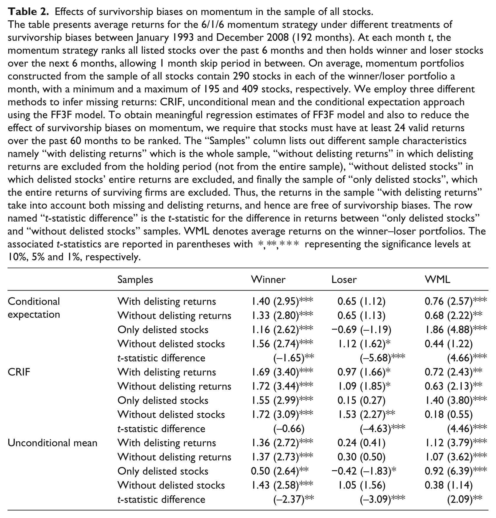
In the sample of only stocks that still survive by the end of December 2008, the average WML return is 0.44% per month with the t-statistic of only 1.22, not significant even at the 10% level. In contrast, the average return in the sample of only delisted stocks is 1.86 ( t-statistic = 4.88), which is economically and statistically strong. The last row reports the t-statistic of the difference between “without delisted stocks” and “only delisted stocks”. Consistent with Eisdorfer (2008), the t-statistic of the difference is 4.66, which is statistically significant at the 1% level, and indicating that delisted stocks contribute a crucial component in the average return of momentum portfolios.
A similar picture is also seen in the CRIF and unconditional mean methods. For the CRIF method, the inclusion of delisting returns boosts the average WML return by 9 bps per month (or 1.08% per year). The WML t-statistic difference between “without delisted stocks and “only delisted stocks” is 4.46, which is also statistically significant at the 1% level. For the unconditional mean method, the average WML return in the “without delisted stocks” group is still economically and statistically small, with 0.38% per month compared with 0.92% per month in the sample of “only delisted stocks”. These findings show that a great portion of momentum profitability is attributable to delisted stocks and their delisting returns. As we argued in the introduction, this reliance on delisted stocks indicates that momentum trading strategies may not be investible due to the constraint of short-selling troubled stocks that are near the end of their listings.
4.2 Evidence in the sample of Top300 stocks
Despite the omission of delisting returns, previous research in the Australian market generally finds that momentum is strong in the largest stocks by market capitalization. This suggests that delisted stocks may play a less important role in the largest group. Consequently, we repeat the above exercise to examine the effect of survivorship biases on average momentum profits in various groups of stocks and report results in Table 3.
Effects of survivorship biases on momentum in the Top300 stocks.
The table presents average returns for the 6/1/6 momentum strategy under different treatments of survivorship biases between January 1993 and December 2008 (192 months). At each month t, the momentum strategy ranks stocks in the Top 300 by market capitalization over the past 6 months and then holds winner and loser stocks over the next 6 months, allowing 1 month skipping period in between. As we group stocks into quintiles, the number of stocks in each winner/loser portfolio is maintained to be 60 stocks per month. We employ 3 different methods to infer missing returns: CRIF, unconditional mean and the conditional expectation approach. To obtain meaningful regression estimates of FF3F model and also to reduce the effect of survivorship biases on momentum, we require that stocks must have at least 24 valid returns over the past 60 months to be ranked. The “Samples” column lists out different sample characteristics namely “with delisting returns” which is the whole sample, “without delisting returns” in which delisting returns are excluded from the holding period (not from the entire sample), “without delisted stocks” in which delisted stocks’ entire returns are excluded, and finally the sample of “only delisted stocks”, which entire returns of surviving firms are excluded. Thus, average returns in the sample “with delisting returns” take into account both missing and delisting returns, and hence are free of survivorship biases. The row named “t-statistic difference” is the t-statistic for the difference in returns between “only delisted stocks” and “without delisted stocks” samples. WML denotes average returns on the winner-loser portfolios. t-statistics are reported in parentheses with *,**,*** representing the significance levels at 10%, 5% and 1%, respectively.
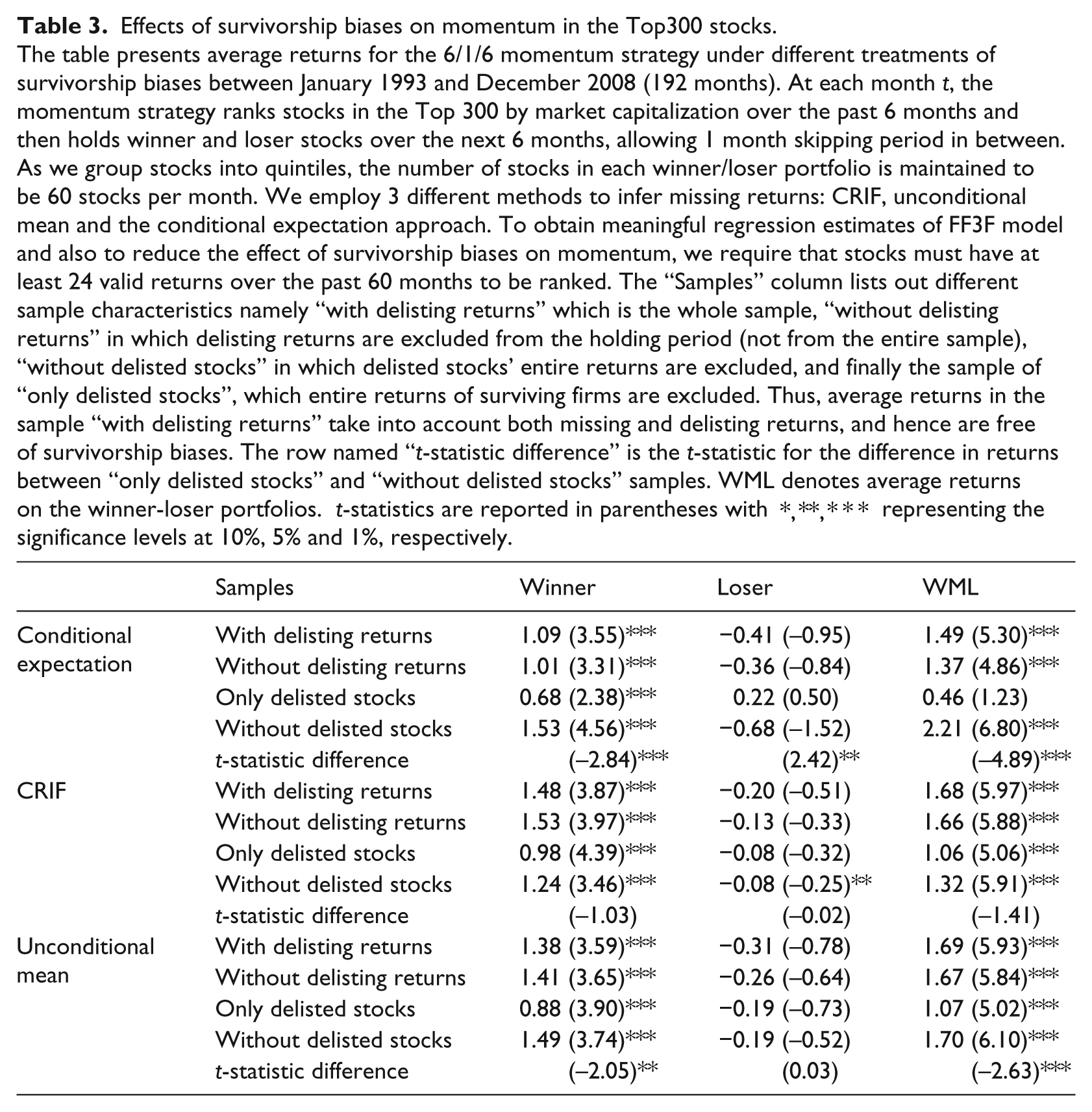
The overall picture is that the average momentum profit is economically and statistically large in all samples and for all methods of inferring missing values. When delisting returns are included in the holding period, momentum portfolios earn the highest return under the unconditional mean approach with 1.69% per month (t-statistic = 5.93) whereas the conditional expectation method gives the lowest average return of 1.49% per month (t-statistic = 5.30). When delisting returns are excluded, the average WML return marginally reduces to 1.66% and 1.67% per month for the CRIF and unconditional mean approaches, respectively. In contrast, the reduction in momentum returns from the conditional expectation approach is 12 bps per month (or 144bps per year), which is economically significant. This reduction indicates that missing delisting returns will also drive down momentum profitability among the largest stocks.
In contrast to the all stocks sample where momentum strategies benefit from bankrupt loser stocks, momentum portfolios in the Top300 have losers that are less likely to go bankrupt. The last three rows of each box of Table 3 show a striking result that delisted stocks (i.e. their entire lives’ returns) play a negative role to the average momentum profit. For the conditional expectation method, the average WML return in the sample “without delisted stocks” is 2.21% per month, much higher than 0.46% per month ( t-statistic = 1.23) in the “only delisted stocks” sample. The t-statistic difference in returns between “only delisted stocks” and “without delisted stocks” samples is −4.89, which is negative and statistically significant. We also see similar pictures in the CRIF and unconditional mean methods. Consequently, surviving stocks contribute more to the average momentum profit in the Top300. This is in stark contrast with Eisdorfer (2008) although Eisdorfer does not investigate the robustness in different size subsamples.
We also note that, in the Top300, a small portion of momentum returns comes from the loser portfolio. For example, under the conditional expectation approach, only 27.5% (
A note on the ex-post examination of delisted stocks
Except for the average return in the sample “with delisting returns” (the first rows of Tables 2 and 3), all results are ex-post investigations. The purpose is to show that delisted stocks and their delisting returns can have a non-trivial effect on the momentum profitability. As delisted stocks are risky, especially for bankruptcy reasons, readers may wonder how these results would help investors to construct momentum strategies that are ex ante less exposed to the risk of delisted stocks.
Although it is beyond the scope of the current study to employ likelihood measures to predict bankruptcies such as the Altman (1968)’s Z score, we find no immediate needs for that. Since delisted stocks play little role, if not a negative role, in determining the average momentum return in the Top300, an easy recommendation for both researchers and practitioners would be to construct momentum portfolios in the largest stocks. For practitioners, trading momentum in the Top300 gives them a higher return, which is also less exposed to the risk of holding stocks with high delisting possibilities. For academics who try to explain the momentum effect, we argue that they now have a bigger task in explaining the robustness of momentum effects in the Top300 in which the average WML return is much higher than in the U.S. markets. The general consensus in the U.S. evidence is that momentum portfolios earn an average return of about 1.13% per month from 1990 to 2009 and the strategy relies heavily on the group of small stocks (Hong et al., 2000; Jegadeesh and Titman, 2011). Since the ASX Top300 contains the largest stocks that are less exposed to liquidity risks, the momentum effect in Australia is actually more puzzling. Although it is beyond the scope of this study to investigate alternative explanations of momentum (which is still an ongoing debate in the literature), our current contribution is to show that delisted stocks are not the driver of momentum effects in Australia.
4.3 Bankruptcy and merger momentum
Table 4 reports the average 6/1/6 momentum return in the samples of bankrupt and merged firms. If returns on bankruptcy stocks drive momentum profits, we should see the average return without bankruptcy stocks to be lower than that in the sample of only bankruptcy stocks. Indeed, this is the picture in all stocks sample (panel A). The average WML return for bankrupt firms only is 1.14% per month (t = 4.16), which is economically and statistically significant. When we exclude bankruptcy stocks, the average momentum profit drops to 0.65% per month, with the associated t-statistic of 1.93, significant only at the 10% level. The difference in returns between the two samples is −0.49% per month, statistically significant at the 10% level (the third row).
Merger and bankruptcy effects.
This table reports average momentum returns in the samples of bankrupt and acquired firms. The “Without mergers” sample does not contain stocks delisted due to mergers and acquisitions (M&A). The “Only mergers” sample consists of stocks delisted due to M&A reasons. “Difference” is the average difference between “Without mergers” and “Only mergers”. Bankruptcy samples have similar definitions. We employ the conditional expectation approach to infer missing returns during the holding period. To obtain meaningful regression estimates of FF3F model and also to reduce the effect of survivorship biases on momentum, we require that stocks must have at least 24 valid returns over the past 60 months to be ranked. t-statistics are reported in parentheses with *,**,*** representing the significance levels at 10%, 5% and 1%, respectively. Panel A shows results in the sample of all stocks while panel B reports results in the sample of Top300 stocks by market capitalization.
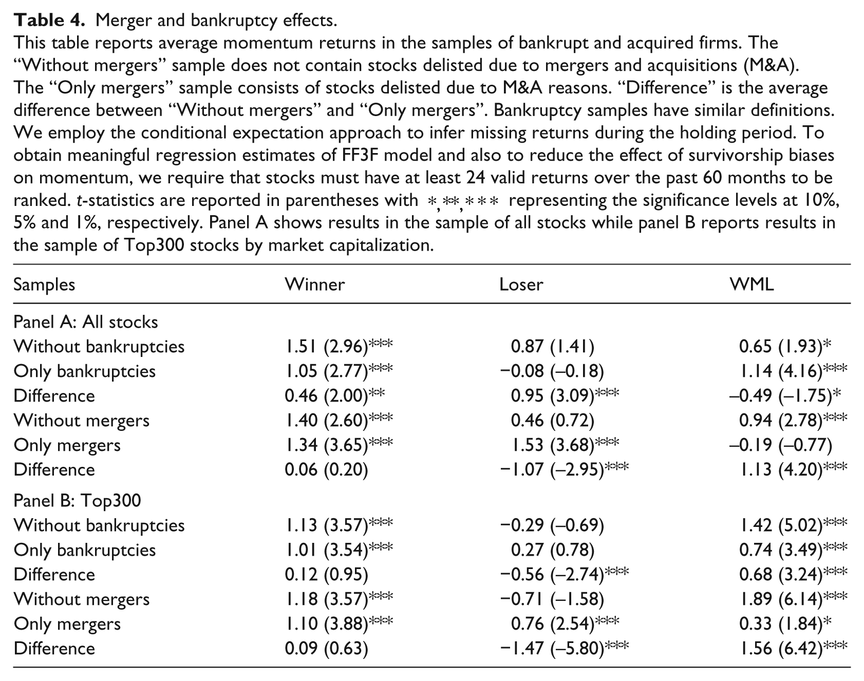
The profit of merger momentum is, on the other hand, negative 0.19% per month with the insignificant t-statistic of −0.77. If we exclude merged stocks from the sample, the average momentum return is 0.94% per month (t=2.78), which is even higher than the full-sample momentum profit of 0.76% per month (first row of Table 2). Also in contrast to the bankruptcy effect, the average WML profit without mergers is actually 1.13% higher than the “only mergers” sample. These findings indicate that the contribution of merged firms in the All Stocks sample is much less than that of bankrupt firms and the delisting effect documented in Table 2 is almost entirely due to bankruptcy stocks.
Panel B of Table 4 shows results in the Top300 by market capitalization. Consistent with Table 3, including delisted firms in the momentum portfolio actually reduces the average profit. First, the average WML return in the group of bankruptcy firms only is 0.74% per month (t =3.49), which is much lower than the full-sample profit of 1.49% per month in Table 3. Also in contrast to panel A, the difference in WML average returns between “without bankruptcies” and “only bankruptcies” samples is positive 0.68% per month. In particular, bankrupt loser stocks in the Top300 now have the positive average return of 27bps per month, which drives down the average momentum profit. Thus, bankruptcy stocks have negative effects on momentum in the Top300.
Second, merged firms also have a negative impact on momentum effects. The average WML profit without mergers is 1.89% per month (t = 6.32), which is 40 bps higher than the average whole-sample momentum return and 1.56% higher than the average “only mergers” profit. This is because, compared with the “without mergers” group, merged winners in the Top300 earn a lower average return while merged losers enjoy a much higher average return during holding periods, causing the average WML return to be lower. Consequently, mergers play a negative role in contributing to the momentum profitability in the Top300.
Overall, panel B of Table 4 shows that if we aggregate all Top300 stocks together in the actual momentum portfolio (the first row of Table 3), the average WML return will reduce due to the negative contribution of bankruptcy and merged stocks. As argued by Eisdorfer (2008), merged firms usually receive their first bids that cause price jumps during the ranking period. Those merged winners therefore have lower subsequent returns in the investment period. On the other hand, merged losers have a period of poor performance, which makes them losers at the end of ranking periods, and subsequently receive the first bid during the holding period, causing relatively high returns. This intuition explains the smaller contribution of merged stocks to the overall momentum profitability.
4.4 Delisting effect on various momentum portfolios
In order to show that the above results are not specific to the 6/1/6 strategy, we repeat the exercise in Table 2 for various combinations of ranking and holding periods and report results in Table 5. Panel A shows consistent results for the sample of all stocks. First, the inclusion of delisting returns in the investment period increases average profits of all strategies by approximately 10 bps per month (or 120 bps per year). Second, the effect of delisted stocks is positive and statistically significant everywhere. Comparing Tables 2 and 5, we can see that the 6/1/6 strategy yields the most profitable momentum portfolio. The 12/1/12 strategy, which ranks stocks over the last 12 months, and then holds WML portfolios for the next 12 months with one month skipping period, is the worst strategy, yielding −8 bps per month although it is not statistically significant. Nevertheless, our conclusions that most of the momentum profitability is attributable to returns on delisted stocks still hold in all strategies. The average momentum return in the sample of only delisted stocks ranges from 0.74% to 1.09% per month, which are all statistically significant at least at the 5% level. In addition, differences between “only delisted stocks” and “without delisted stocks” momentum returns are all positive and statistically significant at the 1% level.
Effects of delisted stocks on various momentum strategies.
The table presents average winner-minus-loser returns on K/I/J momentum strategies under different treatments of survivorship biases between January 1993 and December 2008 (192 months). At each month t, the momentum strategy ranks stocks over the past K months and then holds winner and loser stocks over the next J months, allowing 1 month skipping period in between. The construction of this table is similar to that of Tables 2 and 3. We employ the conditional expectation method to infer missing returns during holding periods. The average returns in the sample “with delisting returns" take into account both missing and delisting returns, and hence are free of survivorship biases. The row named “t-statistic difference" is the t-statistic for the difference in returns between “only delisted stocks" and “without delisted stocks" samples. Panel A shows results in the sample of all stocks while panel B limits the sample to the Top300 by market capitalization. t-statistics are reported in parentheses with *,**,*** representing the significance levels at 10%, 5% and 1%, respectively.

Similar to Table 3, those findings are reversed in the Top300 although the effect of delisting returns is still economically unchanged. Having a complete dataset with delisting returns can improve the average momentum profit in all samples and strategies, as evidenced in the first two rows of panel B. We can see that, in contrast to panel A, momentum returns in all strategies are economically and statistically significant. The 6/1/6 strategy still has the highest average return with 1.49% per month (Table 3) and the 12/1/12 still has the lowest average return with 0.80% per month.
For all strategies reported in the panel B of Table 5, average momentum returns in the sample of “only delisted stocks” are all much lower than those in the sample “without delisted stocks”. Except for strategies with a 3-month holding period, average returns on momentum strategies in the sample of only delisted stocks are either negative or economically small. Also in contrast to panel A, differences between momentum returns in “only delisted stocks” and “without delisted stocks" samples are all negative and statistically significant at least at the 1% level. These findings provide another support to our earlier conclusions that the momentum effect in the Top300 is not attributable to the effect of delisted stocks.
5. Conclusion
By employing a new dataset that incorporates hand-collected delisting returns, we provide the first out-of-sample test of the joint effects of delisting and missing returns on momentum. Consistent with the U.S. evidence, we find that momentum profits rely heavily on delisted stocks and their subsequent delisting returns. However, this effect is reversed in the Top300 by market capitalization, in contrast to the U.S. findings. Since delisted stocks play little role, if not a positive role, in driving the average momentum return in the Top300, an easy recommendation for both researchers and practitioners would be to construct momentum portfolios in the largest stocks. For practitioners, trading momentum in the Top300 gives them a higher return, which is also less exposed to the risk of holding stocks with high delisting possibility. For academics who try to explain momentum, we argue that they have a bigger task in explaining the robustness of momentum in the Top300 in which the average WML return is much higher than in the U.S. markets. Since the Top300 group contains the largest stocks that are less exposed to liquidity risks, the momentum effect in Australia is more puzzling.
Footnotes
Appendix: Constructing Fama and French’s (1993) SMB and HML factors
The three factors of Fama and French (1993) consist of market risk factor (R m −R f ), the size factor (SMB) and the book-to-market factor (HML). SMB, small minus big, captures the premium that small stocks earn over large ones while HML, high minus low, captures the premium that value stocks earn over growth stocks. The Fama–French factors are not readily available in Australia. We follow the methodology of Fama and French (1993) and construct the common risk factors. To ensure that the factors are not affected by the methods used to account for missing returns as outlined in Section 3.4, missing returns are kept as missing.
To construct the size factor, in June of each year t from 1986 to 2008 all listed stocks covered in Aspect database are ranked by market capitalizations. We then assign all stocks with market capitalization higher than the median of ASX market capitalization into big portfolios, B, and the rest into small portfolios, S. To construct the book-to-market factor, all stocks are ranked based on book-to-market values at the fiscal year end (i.e. June). To avoid undoing weight on small stocks, we follow Fama and French (2012) and compute book-to-market breakpoints in the group of large stocks. We exclude all stocks with negative book values of equity. The stocks are categorized such that the first 30% of stocks (growth stocks) has the lowest book-to-market ratios, L; the next 40% of stocks is assigned to medium portfolio, M; and the remaining 30% of stocks (value stocks) comprise the high book-to-market, H, portfolio.
In the next step, we construct six intersection portfolios (S/L, S/M, S/H, B/L, B/M and B/H). These portfolios are held for 12 months and monthly value-weighted returns on those 6 portfolios are computed from July of year t to June of year t+ 1. The SMB and HMl factors are then calculated as follows:
Final transcript accepted 27 November 2014 by Karen Benson (AE Finance).
Funding
This research received no specific grant from any funding agency in the public, commercial or not-for-profit sectors.