Analysis of Roadway Grade Estimations From Global Positioning Systems and Barometer Measurements

Abstract

Roadway grade is used as an input variable for several highway analysis tasks, including evaluating curve margin-of-safety, applying safety prediction models, assessing the adequacy of sight distance, and maintaining state roadlog databases. However, collecting accurate grade data is often expensive owing to the need to obtain field measurements or review as-built plan sets. Agencies would benefit from the development of a method to compute roadway grade from an automated data collection system. This paper documents a comparison of roadway grade estimations computed from global positioning system (GPS) and barometric altimeter data streams obtained during test drives on highway segments of interest. To calibrate the estimation method, the authors obtained ground-truth grade measurements collected from the field and then modeled those measures as responses in a time series model with the two data stream types as explanatory variables. The authors found that for several applications, the elevation data obtained from GPS were adequate to obtain reasonable estimates, but such estimations could be improved with a supplemental data stream from a barometer.

Keywords

data and data science geographic information science GPS data

Roadway grade is a variable of interest for several applications, including roadlog database management, pavement management, sight distance analysis, and roadway safety analysis. Grade has been shown to be a relevant variable to the analysis of margin of safety of horizontal curves ( 1 , 2 ) and is also included in safety prediction models for several roadway facility types, especially rural highways ( 3 ). However, grade data can be expensive to obtain because they are often not included in roadlog databases, and therefore must be field-measured, obtained from as-built plan sets, or computed from contour maps.

Guidance exists to assist practitioners in determining whether a horizontal curve of interest needs a surface treatment to increase the pavement friction supply ( 2 , 4 ). The underlying principle of this guidance is margin-of-safety analysis, which involves computing the difference between friction supply (which depends on pavement skid resistance) and friction demand (which depends on vehicle speed, curve radius, superelevation rate, and grade). The guidance has been assembled ( 5 ) in the form of a spreadsheet program that calls for the following curve geometry attributes as inputs to conduct a margin-of-safety analysis: radius, superelevation rate, deflection angle, and grade.

In this paper, the authors document an analysis of options to extract roadway grade from a data stream. The authors analyzed data streams from a global positioning system (GPS) receiver and a barometric altimeter, and also considered the option of using an inclinometer. The paper consists of three parts. The first part of the paper provides a literature review. The second part presents the data analysis and results. The third part states the conclusions.

Literature Review

Various applications require the collection and analysis of roadway geometry data streams. Some of these applications include maintaining roadway inventory databases, analyzing roadway operational and safety performance, modeling vehicle dynamics for the purpose of assessing occupant comfort, facilitating implementation of connected or automated vehicle technology, and assessing the adequacy of traffic control devices or pavement friction at key points on the roadway such as horizontal curves. For the purpose of conducting a margin-of-safety analysis of a curve, grade is included in the calculation of side friction demand as follows ( 6 ):

M . S . = f_{S} - f_{D}

(1)

with

f_{D} = \frac{v^{2}}{g R_{p}} \cos (\frac{e}{100}) - \sin (\frac{e}{100}) \cos G

(2)

where

M.S. = margin of safety;

f_s = side friction supply;

f_D = side friction demand (lateral acceleration divided by g);

v = vehicle speed, ft/s;

g = gravitational constant (= 32.2 ft/s²);

R = curve radius, ft;

e = superelevation rate, %; and

G = vertical grade (ft/ft).

Based on Equations 1 and 2, the effect of grade on margin of safety is notable but minor compared with the other geometric variables. Including grade in the computation of margin of safety will improve the analysis results if the grade data are available.

The Highway Safety Manual ( 3 ) includes a crash modification factor (CMF) for grade and terrain on rural two-lane highways. This CMF consists of the following values:

• Level grade (|G| ≤ 3%): 1.00;

• Moderate terrain (3% < |G| ≤ 6%): 1.10; and

• Steep terrain (|G| > 6%): 1.16.

These values are used as multiplicative adjustment factors to increase the predicted crash frequency by 10% for highways with moderate terrain or 16% for highways with steep terrain, without regard to the sign of the grade (uphill or downhill).

The literature includes discussion of three data sources that can be used to compute roadway grade. These data sources include

• Inclinometers, which measure angles for one or more axes of a moving vehicle;

• GPS receivers, which provide latitude, longitude, and elevation coordinates at a specified time interval for the purpose of computing velocity and position; and

• Barometric altimeters, which use measurements of air pressure and temperature to provide altitude values.

Issues with computing roadway grade from these sources are described in the following three sections. A more detailed discussion is provided elsewhere ( 7 , 8 ).

Inclinometer

An inclinometer can be used to measure angles of rotation about the vehicle’s pitch axis as shown in Figure 1. The pitch axis is represented as the circular symbol and runs into the page. Figure 1 illustrates the combined contributions of roadway grade (θ) and vehicle pitch (λ) to the reading that would be obtained from an inclinometer. In the example shown, the inclinometer would measure the combined angle θ + λ, which is greater than the roadway grade θ.

Figure 1.

Vehicle pitch angle and grade.

Hashemi et al. described the relationship between vehicle pitch angle, roadway grade, longitudinal acceleration and braking, and vehicle characteristics including suspension stiffness and weight distribution ( 10 ). They modeled the vehicle using sprung-mass kinematics and derived a system of equations to describe vehicle roll and pitch. They observed that the equations describing rotation about the pitch axis include both angles θ and λ, such that it is necessary to use height sensors on all four wheels to measure suspension displacements and decouple the two angles. By using an instrumented vehicle that included these sensors and other components, they were able to measure vehicle pitch, λ, and compute roadway grade, θ.

Hashemi et al. tested the accuracy of their grade measurements by deliberately inducing error through longitudinal acceleration and braking, and found that the grade-calculation algorithm still produced accurate results. In one example test run, they showed that the difference in suspension displacement between the front and rear axes was about 3 to 4 in. Their instrumented vehicle had a length of about 9 ft between the two axes; for this length, a 3.5-in. increase in displacement between the axes would increase the vehicle pitch angle by about 1.9°, or overestimate the roadway grade by about 3.2% (i.e., a grade of 5% would be computed as 8.2%). Their instrumented vehicle system was able to compensate for this error source by measuring longitudinal acceleration and incorporating it into the calculations.

GPS Receiver

GPS receivers provide data sentences with standard formats that are specified by the National Marine Electronics Association ( 11 ). Two of the sentence formats include RMC, which provides position, speed, and heading; and GGA, which provides altitude. It is generally suggested that GPS provides excellent position data, but the error for GPS-measured altitude is roughly 50% higher than for GPS-measured position ( 12 ).

Vahidi et al. investigated methods to use GPS-measured altitude (or elevation) data to compute roadway grade ( 13 ). They showed that the raw elevation data are generally accurate but often have errors of about 25 ft because of measurement fluctuations (see Figure 2). To improve the computed altitude measurements, they suggested a modeling method called recursive least squares with forgetting. Their comparison of estimated and actual grade is shown in Figure 3.

Figure 2.

Accuracy of raw GPS-measured elevation ( 13 ).

Figure 3.

Accuracy of improved GPS-computed grade ( 13 ).

Barometer

Yazdani et al. evaluated the accuracy of roadway grade measurements obtained from a GPS receiver with a built-in barometric altimeter ( 14 ). They discussed several error sources that can combine to yield uncertainty as high as about 33 ft for GPS-measured horizontal position, and observed that elevation measurements are typically subject to more random error than horizontal position measurements. To improve elevation estimates, they suggested using a GPS receiver with a barometric altimeter. They also acknowledged that differential GPS systems can yield more precise elevation measurements but at significant cost (e.g., $15,000 for one system).

Yazdani et al. suggested that a combination GPS/barometer device could be used to obtain accurate measurements of grade if repeated measurements are conducted on the roadway. They suggested that for roadway segments of about 500 ft in length, a sample size of 22 data collection runs would yield grade confidence intervals of about ±0.5%. The device that they used had a refresh rate of 1 Hz; they suggested that combining data from multiple devices to increase the number of data points would allow for fewer runs to be conducted. It must be noted that Yazdani et al. were seeking repeatability in raw location measurements, and although absolute errors in the range of 33 ft may occur between runs when notable time has elapsed or atmospheric conditions have changed, it is likely that measurements over a short sampling period would vary significantly less, such that computations of relative change in elevation would be repeatable.

Discussion

Based on the results of the literature review, consideration of costs for the different data collection devices, and the need to ensure portability of the data collection system, the authors explored the use of elevation data from a GPS receiver with a built-in barometric altimeter. The authors conducted a preliminary analysis of altitude change measurements obtained from a combined GPS/barometer at 1-Hz intervals, and also aggregated and averaged the measurements as follows:

• Aggregate the GPS-based elevation change estimates over a 3-s interval.

• Aggregate the barometer-based elevation change estimates over a 3-s interval.

• Average the 3-s aggregated measurements from both data sources.

To preliminarily assess the potential use of barometers, the authors conducted an analysis of error in altitude measurements obtained from a barometric altimeter. The basis for calculating elevation change using a barometer is the hypsometric equation, which derives directly from the hydrostatic equation for the ideal gas law ( 15 ). This relationship is shown in Equation 3,

Δ h = \frac{R_{d} {\bar{T}}_{v}}{g} \ln (\frac{p_{2}}{p_{1}})

(3)

where

Δh = change in altitude, m;

p₁, p₂ = pressures at points 1 and 2 (p₁ < p₂), Pa;

g = gravitational constant (= 9.81 m/s²);

R_d = dry air gas constant (= 287.04 J/kg/K); and

${\bar{T}}_{v}$ = average virtual temperature of the air layer of thickness Δh, K.

After substituting constants and converting units, Equation 3 simplifies into the working version shown in Equation 4,

Δ h = 53.352 \ln (\frac{p_{2}}{p_{1}}) ({\bar{T}}_{Fahrenheit} + 459.67)

(4)

where Δh = change in altitude, ft.

The differential of the above measurement is defined as follows:

err (Δ h) = \frac{\partial Δ h}{\partial {\bar{T}}_{Fahrenheit}} Δ {\bar{T}}_{Fahrenheit} + \frac{\partial Δ h}{\partial p_{1}} err (p_{1}) + \frac{\partial Δ h}{\partial p_{2}} err (p_{2})

(5)

err (Δ h) = 53.352 [\ln (\frac{p_{2}}{p_{1}}) Δ {\bar{T}}_{Fahrenheit} + (\frac{1}{p_{1}} + \frac{1}{p_{2}}) ({\bar{T}}_{Fahrenheit} + 459.67) err (p)]

(6)

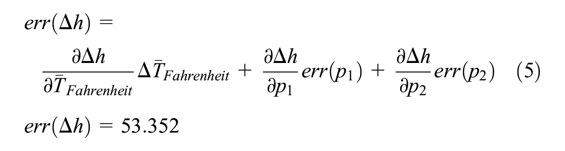
The last term is the maximum case of the general form $(\frac{err (p_{1})}{p_{1}} \pm \frac{err (p_{2})}{p_{2}})$ .

The following sensitivity analysis explores various scenarios of the application of the calculations outlined above, when a stream of digital data is obtained from a barometer, identifying some potential limitations with precision of the readings. An estimate for the amount of error in a pressure reading was obtained from a barometer from an Android S6 device running the Physics Toolbox Suite app that was developed by Vieyra Software ( 16 ). The device was placed untouched on a horizontal surface for 10 s while the signal from the barometer was recorded. The standard deviation of this reading was measured and used as an estimate of err(p). The estimate so obtained was 5.5 × 10⁻⁴ inHg. The plot in Figure 4 illustrates an approximate linear relation between Delta p obtained from the barometer and the corresponding difference in height. This figure shows the “ground-truth” relationship in black, the 95th-percentile frequency band around this ground truth (in dashed gray lines), and two sample noisy signals from the barometer.

Figure 4.

Change in altitude estimated from a change in barometric pressure with two sample noisy signals.

From this figure, it can be seen that each Delta p reading is roughly expected to have the same uncertainty (about 1 ft corresponding error in height difference) when temperature is known with certainty.

Figure 5 shows the same relationship as Figure 4 but with a temperature of 110°F instead of 75°F. The two more relevant results of this change are that the error of the estimation of change in height increases slightly from 1.05 to 1.12 ft; and the slope of the relationship increased slightly as well. At 75°F, this slope was 42.7 ft per 0.04 inHg, but at 110°F it changed to about 45.9 ft per 0.04 inHg. Therefore, the results of the estimation method clearly depend on the temperature at which the data are collected.

Figure 5.

Example of change in altitude estimated from a change in barometric pressure at 110° with two sample noisy signals.

Finally, Figure 6 shows the same relationship as Figure 4 but allowing for the uncertainty associated with temperature. This uncertainty has been fixed at ±10°F, which could be considered a common range in temperatures expected during an 8-h day of data collection. It can be seen that the two most crucial effects of this change were that the average error of the estimation almost doubled from 1.05 to 2.00 ft; and that more uncertainty was associated with bigger changes in pressure (i.e., the dispersion increases with increased pressure difference). These two results indicated that having a simultaneous stream from a good instantaneous thermometer would be desirable to increase the accuracy of this estimation. It should be noted that the combined GPS/barometer device used by the authors to conduct the exploration of field-measured elevation values reported altitude, pressure, and temperature on its digital display.

Figure 6.

Change in altitude estimated from a change in barometric pressure.

Data Analysis

This part of the paper describes efforts to develop automated methods to measure roadway grade. The two evaluated data sources include GPS elevation data and elevations measured using a barometer.

GPS provides elevation data and horizontal position data in two separate data sentences, which are designated as GGA and RMC, respectively ( 11 ). As a rule of thumb, it has been suggested that the error in GPS-measured elevation should be assumed to be 50% greater than the error in GPS-measured horizontal position ( 12 ). Barometers (or barometric altimeters) provide measurements of elevation based on atmospheric pressure. For the purpose of computing roadway grade, elevation data need to be accurate in the relative sense (i.e., the change in elevation between subsequent points) but not in the absolute sense.

Exploratory Analysis

Figure 7 shows a comparison of elevation data measured from a device that contains a GPS receiver and a barometer. The GPS-measured elevation is shown in red and the barometer-measured elevation is shown in black. The two data series track each other, but with some error present in both.

Figure 7.

Comparison of barometric and GPS elevation.

Figure 8 shows an additional comparison of the data series with a vertical shift of 79.6 ft and a signal amplification of 14% on the barometer data series. As shown, the data series compared favorably when adjusted.

Figure 8.

Adjusted comparison of barometric and GPS elevation.

The authors obtained ground-truth grade measurements collected from the field at 100-ft increments at three sites (Blue Ridge Drive, Koppe Bridge Road, and Dogwood Trail, all in Brazos County, Texas). The following process was used to compute the plotted grade measurements for the GPS and barometer devices:

Tabulate the elevation measurements that were recorded by the devices. These measurements were in increments of 20 to 30 ft, as influenced by test vehicle speed and device frequency.

Compute grade values between successive points as the difference in elevation divided by the distance traveled between points.

Interpolate the computed grade values to obtain grade estimates at the 100-ft increment points that correspond to the ground-truth grade data.

A comparison of GPS- and barometer-computed grade with ground-truth grade is shown in Figure 9. It can be seen that the grade values from both data streams generally track the ground-truth grade, but with some uncertainty and some unexpected spikes. The sources of these spikes could include vehicle bounce (which would cause vertical shifts) or device reporting latency (which would cause horizontal shifts). However, it appeared that either data source could be adjusted to provide grade measurement of adequate accuracy for the purpose of conducting a curve margin-of-safety analysis.

Figure 9.

Comparison of measured and ground-truth grade.

Modeling Grade as a Function of Device Data

The authors developed time series models of the road grade as a function of the data streams, GPS- and barometer-based, obtained from a device capable of producing both readings simultaneously. The ground-truth grade readings were then analyzed in conjunction with the device-based estimates (i.e., the three streams shown in Figure 9).

Modeling Framework

The authors specified a mixed-effects model for the data streams allowing for time series characteristics. The general form is shown in Equation 7.

G_{ij} = (X_{ij} \cdot ML) \cdot β + ρ_{i} + ε_{ij}

(7)

where

G_ij = grade at the ith site at jth reading point;

X_ij = set of explanatory factors at ith site and jth reading, modeled as fixed underlying parameters;

ML = matrix of lead/lag operators;

β = coefficients correspondent to the explanatory factors;

ρ_i = random intercept for ith site; and

ε_ij = error structure of the residual errors, potentially including codependence relationship within site i and reading j.

The two main features of the model structure in Equation 7 are the application of a matrix of lag operators and the ability to incorporate codependence relationships in the error structure.

Matrix of Lead/Lag Operators

The matrix of lead/lag operators is partitioned into two subsets. Given that there are two explanatory variables (i.e., GPS and barometric grade estimates, respectively), the matrix is of dimension 2 × (m + n) as follows:

ML = [M L_{GPS} | M L_{Barometer}]

(8)

The first partition corresponding to GPS readings is a matrix of dimensions 2m such that,

M L_{GPS} = [\begin{matrix} \begin{matrix} L^{0} \\ 0 \end{matrix} & \begin{matrix} L^{1} \\ 0 \end{matrix} \dots \begin{matrix} L^{m - 1} \\ 0 \end{matrix} \begin{matrix} L^{m} \\ 0 \end{matrix} \end{matrix}]

(9)

The second partition corresponding to barometer readings, is a matrix of dimensions 2n,

M L_{Barometer} = [\begin{matrix} \begin{matrix} 0 \\ L^{0} \end{matrix} & \begin{matrix} 0 \\ L^{1} \end{matrix} \dots \begin{matrix} 0 \\ L^{n - 1} \end{matrix} \begin{matrix} 0 \\ L^{n} \end{matrix} \end{matrix}]

(10)

The lag operator is defined for a given time series as follows:

L \cdot X_{t} = X_{t - 1}

(11)

A lead operator is defined as follows:

Ld \cdot X_{t} = X_{t + 1}

(12)

The authors considered values of m and n in the above definitions of up to five in the modeling process, for both lead and lag operators. As described later, an examination of the relationship between the ground-truth values and the device estimates exhibited a lag in the devices (i.e., inflections of grade in the terrain appeared to show up in the device streams at a slight delay, such as in Figure 10). For this reason, the final model described below included only lead operators and no lag operators.

Figure 10.

Comparison of three grade measurement time series at Blue Ridge site.

Codependence Error Structure

When handling a data stream collected as a time series (i.e., a sequence of data points close in time), it is very important to explicitly consider the likely codependence between observations as a function of their proximity in time. This need is more critical for situations of higher granularity in the time scale as is the case of the GPS and barometer data. The mixed-effects framework proposed by Pinheiro and Bates is compatible with these considerations and allows the implementation of time series methods to account for error correlation structures ( 17 ). The general modeling structure explicitly accounts for three types of data feature: (1) variables treated as fixed effects, which are expected to have “global” effects that are not time-dependent (e.g., a set of device readings and corresponding lead/lag operators); (2) variables treated as random effects, which can account for clusters or hierarchical structures in the data (such as in this case different data streams collected at three different sites); and (3) specific types (i.e., structures) of time-dependence in the errors for a time series at any level of the dataset hierarchical structure.

For this particular analysis, the authors implemented and tested the performance of an error structure at the lowest level of the hierarchical structure in the data. The methods implemented were those widely accepted and used in time series modeling originally proposed by Box et al. ( 18 ) and Tiao and Box ( 19 ).

The general model framework is known as auto-regressive moving average modeling (ARMA). This error specification accounts for the degree to which a given value in the time series is determined by prior values in the time series. Equation 13 shows the general form of the error structure under the ARMA specification.

ε_{ij} = \sum_{u = 1}^{p} δ_{u} \cdot L^{u} ε_{ij} + \sum_{v = 1}^{q} θ_{v} \cdot L^{v} φ_{ij} + φ_{ij}

(13)

where

ε_ij = residual at site i and reading j;

δ_u = coefficient for L^uε_ij in the combination of lagged residuals in the ARMA model;

θ_v = coefficient for L^vφ_ij in the combination of lagged residual nuances in the ARMA model;

L ^uε_ij = lag u of residual (i.e., $L^{u} ε_{ij} = ε_{i, j - u}$ );

L ^vφ_ij = lag v of residual nuance parameter (i.e., $L^{v} ϕ_{ij} = ϕ_{i, j - v})$ ;

p = largest lag in the autoregressive part of the ARMA model; and

q = largest lag in the moving average part of the ARMA model.

The error structure of the model is such that $ϕ_{ij} ~ N [0, σ_{0}^{2}]$ . The expected variance is estimated along with the rest of parameters in the model.

The authors conducted regression analysis using open source statistical software and packages ( 19 – 21 ) to derive a smooth model to estimate grade from GPS- or barometer-based grade measurements. The analysis focused on ground-truth grade as the response variable and device-based grade calculations as predictor variables. A preliminary analysis without leads, lags, or error correlation structure showed that GPS-measured grade values had an average error of 2.25% with no significant differences found between the three test sites. A model using both GPS-based grade values and barometer-based grade values had an average error of 2.06%. These models are described as follows:

G = 0.471 G_{GPS}

(14)

G = 0.296 G_{GPS} + 0.225 G_{barom}

(15)

where

G = ground-truth grade, %;

G_GPS = GPS-based grade, %; and

G_barom = barometer-based grade, %.

Both models showed that a downscaling of the device-based values was needed to obtain an accurate measurement of grade. The model that used both devices (Equation 15) did have a slightly lower error range than the model that used only GPS (Equation 14), but the small improvement did not justify requiring the use of a barometer.

A comparison of ground-truth, GPS-based, and barometer-based grade measurements suggested that device-based values had the tendency to lag, perhaps owing to device latency or the response of the vehicle’s suspension. This trend is illustrated in Figure 10. To improve the GPS-based estimate of grade, the authors calibrated a model that included two lead operators (to cancel the lag in the series). As mentioned earlier, the research team tested up to five leads and lags but reduced the model by metrics of quality of information (i.e., Akaike information criterion). The most parsimonious model structure is described as follows:

G = b_{0} G_{GPS, 0} + b_{1} G_{GPS, 1} + b_{2} G_{GPS, 2}

(16)

where G_GPS,n = nth GPS-based grade estimate, %.

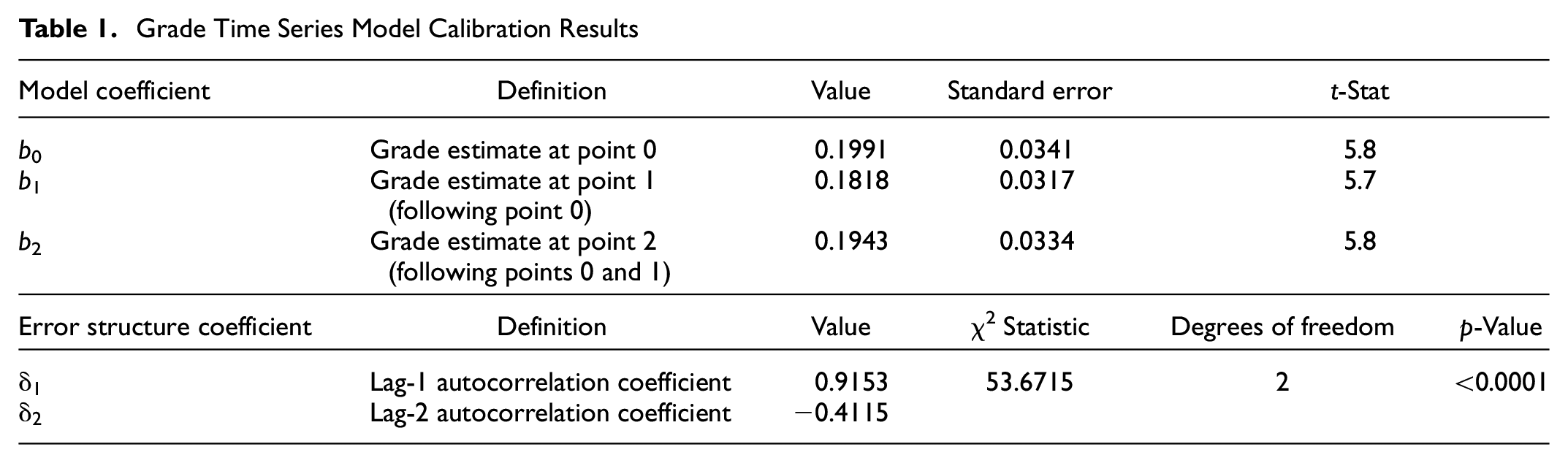
The model calibration results, after adding a codependence structure in the errors, are shown in Table 1, and the calibrated model is described in Equation 17. The error range for this model was found to be 1.63%, a notable improvement on the preliminary model described in Equation 14. Figure 11 shows the actual and estimated grades along the road for the Koppe Bridge site. The estimates are labeled as “GPS alone” for Equation 17 (using GPS data), “Barometer alone” for Equation 17 (using barometer data), and “GPS + barometer” for Equation 15. Figure 12 shows how the estimated grade using Equation 17 compared to the actual grade at the three sites.

Table 1.

Grade Time Series Model Calibration Results

Model coefficient	Definition	Value	Standard error	t-Stat
b ₀	Grade estimate at point 0	0.1991	0.0341	5.8
b ₁	Grade estimate at point 1 (following point 0)	0.1818	0.0317	5.7
b ₂	Grade estimate at point 2 (following points 0 and 1)	0.1943	0.0334	5.8
Error structure coefficient	Definition	Value	χ ² Statistic	Degrees of freedom	p-Value
$δ_{1}$	Lag-1 autocorrelation coefficient	0.9153	53.6715	2	<0.0001
$δ_{2}$	Lag-2 autocorrelation coefficient	−0.4115	53.6715	2	<0.0001

G = 0.1991 G_{GPS, 0} + 0.1818 G_{GPS, 1} + 0.1943 G_{GPS, 2}

(17)

Figure 11.

Performance of grade-calculation model at Koppe Bridge site.

Figure 12.

Comparison of estimated and actual grade.

Summary and Conclusions

The authors examined roadway grade values that were computed from GPS and barometer data streams. They found that the GPS data stream yielded reasonable estimates of roadway grade, which could be improved if supplemented with a barometer data stream. The added precision offered by the barometer data stream was not needed for the purpose of conducting a curve margin-of-safety analysis or applying the CMF in the Highway Safety Manual, but it may be needed for other applications, such as updating state roadlog database files.

A limitation of this study is the small number of locations for which the data were available. The limiting factor was the amount of effort for the data collection and reduction using GPS and barometer data streams and synchronization with the ground-truth dataset. Future work should validate the findings from this research for a broader set of geometric conditions, including broader ranges in superelevation, radius, and multiple reversed horizontal curves. To facilitate adoption of the results from this research, it is also recommended to develop an automated system to collect data and produce the grade estimation in a seamless way.

Footnotes

Acknowledgements

The authors thank the Texas Department of Transportation for sponsoring this research

Author Contributions

The authors confirm contribution to the paper as follows: study conception and design: M. Pratt, R. Avelar; data collection: M. Pratt; analysis and interpretation of results: R. Avelar, M. Pratt; draft manuscript preparation: M. Pratt, R. Avelar. Both authors reviewed the results and approved the final version of the manuscript.

Declaration of Conflicting Interests

The authors declared no potential conflicts of interest with respect to the research, authorship, and/or publication of this article.

Funding

The authors disclosed receipt of the following financial support for the research, authorship, and/or publication of this article: This research was sponsored by the Texas Department of Transportation (Research Project 0-6960).

ORCID iD

Raul E. Avelar

References

Bonneson

Superelevation Distribution Methods and Transition Designs. NCHRP Report 439. TRB, National Research Council, Washington, D.C., 2000.

Pratt

Geedipally

Pike

Carlson

Celoza

Lord

Evaluating the Need for Surface Treatments to Reduce Crash Frequency on Horizontal Curves. Report FHWA/TX-14/0-6714-1. Texas A&M Transportation Institute, College Station, 2014.

Highway Safety Manual . American Association of State Highway and Transportation Officials, Washington, D.C., 2010.

Pratt

Geedipally

Wilson

Das

Brewer

Lord

Pavement Safety-Based Guidelines for Horizontal Curve Safety. Report FHWA/TX-18/0-6932-R1. Texas A&M Transportation Institute, College Station, 2018.

Pratt

Geedipally

Avelar

Horizontal Curve Evaluation Handbook. Report FHWA/TX-19/0-6960-P1. Texas A&M Transportation Institute, College Station, 2020.

Dunlap

Fancher

Scott

MacAdam

Segel

Influence of Combined Highway Grade and Horizontal Alignment on Skidding. NCHRP Report 184. TRB, National Research Council, Washington, D.C., 1978.

Finley

Chrysler

Carlson

Pike

Park

E. S.

Pratt

Avelar

, et al. Traffic Control Device Evaluation Program: FY 2017. Report FHWA/TX-18/9-1001-14-4. Texas A&M Transportation Institute, College Station, 2018.

Pratt

Geedipally

Avelar

Lord

Developing Enhanced Curve Advisory Speed and Curve Safety Assessment Guidelines. Report FHWA/TX-19/0-6960-R1. Texas A&M Transportation Institute, College Station, 2019.

Bae

Ryu

Gerdes

Road Grade and Vehicle Parameter Estimation for Longitudinal Control Using GPS. Proc., Institute of Electrical and Electronics Engineers, Intelligent Transportation Systems, Piscataway, NJ, IEEE, New York, 2001, pp. 166–171.

10.

Hashemi

Zarringhalam

Khajepur

Melek

Kasaiezadeh

Chen

Real-Time Estimation of the Road Bank and Grade Angles With Unknown Input Observers. Vehicle System Dynamics: International Journal of Vehicle Mechanics and Mobility, Vol. 55, No. 5, 2017, pp. 648–667.

11.

NMEA Data. Gpsinformation.org. http://www.gpsinformation.org/dale/nmea.htm. Accessed July 21, 2017.

12.

Altitude Accuracy. http://gpsinformation.net/main/altitude.htm. Accessed July 21, 2017.

13.

Vahidi

Stefanopoulou

Peng

Recursive Least Squares With Forgetting for Online Estimation of Vehicle Mass and Road Grade: Theory and Experiments. Vehicle System Dynamics: International Journal of Vehicle Mechanics and Mobility, Vol. 43, No. 1, 2005, pp. 31–55.

14.

Yazdani

Frey

Sandhu

Road Grade Measurement Using In-Vehicle, Stand-Alone GPS With Barometric Altimeter. Journal of Transportation Engineering, Vol. 139, No. 6, 2013, pp. 605–611.

15.

Wallace

Hobbs

Atmospheric Science: An Introductory Survey. Academic Press, Burlington, MA, 1977.

16.

Physics Toolbox Apps by Vieyra Software. https://www.vieyrasoftware.net/. Accessed August 11, 2017.

17.

Pinheiro

Bates

Mixed-Effects Models in S and S-PLUS. Springer, New York, NY, 2000.

18.

Box

Jenkins

Reinsel

Ljung

Time Series Analysis: Forecasting and Control, 5th ed. John Wiley and Sons, Hoboken, NJ, 2015.

19.

Tiao

Box

Modeling Multiple Time Series With Applications. Journal of American Statistical Association, Vol. 76, No. 376, 1981, pp. 802–816.

20.

R: A Language and Environment for Statistical Computing. http://www.R-project.org. Accessed April 30, 2013.

21.

Bates

Mächler

Bolker

Walker

Fitting Linear Mixed-Effects Models Using LME4. Journal of Statistical Software, Vol. 67, No. 1, 2015, pp. 1–48.