




Abstract
In 2012, California ended Redevelopment Areas (RDAs), which was the state’s primary program for tax increment financing. The state justified its actions based on budgetary issues and lack of evidence as to the program’s effectiveness. Examining exact U.S. Census Bureau tract-level data and in comparison with cohort tracts from 1980 through 2000, this study finds that California RDAs established in the 1990s resulted in minimal positive economic impacts to RDA areas, suggesting that the state may have been correct. Beyond the California issue, this study contributes to the literature by possibly being the first study to examine the general economic impacts of tax increment financing areas.
Introduction
Currently, 48 states have enacted programs that allow local development agencies to finance new projects through tax increment financing (TIF). 1 These programs provide property tax subsidies and bond financing to projects intended to decrease urban blight and increase economic growth. Although there is a large and growing literature on the effects of TIF on property values, despite billions of dollars in tax subsidies annually across the United States, 2 there is scant empirical evidence as to whether TIFs are an effective means of improving the economy of depressed areas.
This study examines the economic impacts of California TIFs, which were operationalized through the Redevelopment Area (RDA) program. From 2010-2011, the California RDA program was estimated to cost $1.7 billion annually. 3 In response to budgetary considerations and lack of evidence on the effectiveness of the program 4 as well as perceived inefficiencies, 5 the California legislature and governor voted in 2011 to end the program, and the constitutionality of this action was later upheld by the California Supreme Court. 6 The program was officially dismantled in February 2012. A significant driver of this decision was a report by the independent California Legislative Analyst’s Office, which, surveying empirical work done on non-California TIFs, concluded that the program did not increase economic development (the report also concluded that reliable empirical studies for California did not exist). 7 Since the California program was the first TIF program to be ended nationally, and as such might serve as a bellwether case for other states with similar budget problems, research into whether this program was actually ineffective (as opposed to being simply a budgetary issue) is of importance.
This study examines the impact of California RDA policies on RDAs at the census tract level, which allows us to be precise about the exact area that makes up an RDA, and its surrounding communities. Individual RDA maps were digitized to create precise areas of RDAs and of their adjoining census tracts. Related economic data from the census for 1980, 1990, and 2000 are used to compare the economic performance of RDAs versus immediately adjacent areas and to the rest of California. A differences-in-differences methodology is used, which allows the comparison of the economic conditions of census tracts within an RDA to tracts right next to an RDA. If the effect of RDA policies is simply to generate a movement of economic activity from areas neighboring RDAs to RDAs proper, we would be able to capture this effect by examining areas surrounding RDAs. The results show that in the 1990s there was little measurable impact of RDAs on RDA area employment, poverty rates, family incomes, rental vacancy rates, and average residential rental rates. There was also little measureable business growth in such areas during the 2000-2009 decade in terms of job creation or business revenues.
Beyond the policy issues related to the California TIF program, this study contributes to the literature by examining the economic impacts of TIFs to local economies. Because TIFs are essentially predicated on tax revenues generated by property valuations, prior research has primarily focused on valuation issues (see Dye & Merriman, 2000, and others). 8 A notable exception is Byrne (2010), who found that aggregate municipal employment in cities having TIFs in Illinois did not experience any statistically significant increase in jobs. This study goes beyond Byrne by examining whether residences and businesses in very specific TIF areas (measured at the census tract level) enjoyed any sort of economic benefits. The policy implications of such economic expansion are clear if unemployment and poverty rates are reduced or incomes are increased. The state fiscal implications are also clear: Residents who earn more income pay more state income taxes and consume more, which increases state/local tax collections. Similarly, firm growth increases state and local tax collections, as well.
Tax Increment Financing and Related Prior Research
Although TIF policies vary by state, the common thread is as follows. An area is created within a city and the base value (or assessed valuation of property) within that area is calculated. Property taxes continue to be levied and the property taxes generated by applying the tax rate to the base value continue to be paid to the local governments. Tax revenues generated from any increased property value within the area are earmarked for the city or for an economic development agency controlled by the municipality. These incremental funds are to be used for public improvements and other economic development programs within the area on a pay-as-you-go basis (i.e., as revenues are generated). For some TIF areas, bonds backed by the projected incremental revenues are issued, which generate funds to make major public investments. When the TIF expires, all property tax revenues go to the city and presumably related bonds have been paid off. TIF sizes can vary from a few blocks to much of a city. TIF areas can be created in anticipation of development or created in response to developer demands. TIF funds are generally used to create infrastructure that would attract additional development.
A number of studies have examined the decision to create TIFs (and the area covered). In a study of TIF adoption in Michigan, Anderson (1990) found that cities with growing populations and growing property values, rather than shrinking cities, were actually more likely to adopt a TIF plan because TIF provides a tool for financing the infrastructure required by growth. Dye and Merriman’s (2000) study of TIF in the six-county Chicago metropolitan area over an 18-year period found that in the 4 years before TIF adoption, property values grew slightly faster in the municipalities that were to later adopt TIF than in those that did not. Luce’s (2003) studies of TIF in Missouri found that it is used primarily in affluent/suburban areas of Kansas City and St. Louis. Byrne (2006) examined TIF adoption in the Chicago metropolitan area and found that although most TIFs were used in older, poorer areas, a significant fraction—about one quarter—was adopted in more affluent areas. These studies are consistent with Merriman (2009), who suggests that TIF is more likely to be adopted in areas suffering mild economic distress than in areas marked by more severe distress. Byrne (2005) determined that in metropolitan Chicago “strategic interaction” (nearby cities adopting TIF) played a significant role in making it likely that a municipality would create a TIF district, a result Anderson and Wassmer (2000) similarly found in the Detroit area.
TIF is generally accompanied by property value growth within the district. In a survey of the literature, Briffault (2010) noted that TIF districts succeed in creating a “solid and robust” revenue base (both property values and retail sales), although there is a large variation in success across districts and it is often debatable whether economic growth that is attributed to the TIF would have occurred anyway. On the other hand, Kelsay (2005), in a survey of TIF districts in Kansas City, found that in many projects actual revenues were significantly below projected revenues, and a survey of TIF districts in Texas (Arvidson, Hissong, & Cole, 2001) found that one in five reported no new business activity attributable to the district.
A number of studies have examined the impact beyond TIF borders. A study of Indiana TIFs by Man and Rosentraub (1998) found that TIF-financed infrastructure investment and improvements had a statistically significant positive effect on median house values in the entire host city. Byrne found that TIFs located in industrial areas were particularly successful in promoting property value growth (2010). On the other hand, Dye and Merriman (2000) found that use of TIF was associated with a larger decline in the property values of municipalities that used TIF compared with those that did not. 9 Arvidson et al.’s (2001) examination of Texas TIFs found that TIF commercial projects do little to add to regional jobs or the tax base, which suggested that TIFs simply redistributed sales within a metropolitan area.
California Redevelopment Areas
The nation’s largest state TIF program was the California RDA program. California invented tax increment financing in 1952 and maintained over 400 RDA districts with an aggregate of over $10 billion per year in revenues, over $28 billion of long-term debt, and over $674 billion of assessed land valuation (as of 2008). 10 California also allowed an RDA to buy and sell property and to use eminent domain to acquire property. The two major advantages of the California RDA program were touted to be selective targeting to encourage economic development and the ability to create affordable housing.
Under the powers granted to them in California redevelopment law, cities could target areas within their jurisdiction for economic development. Establishing an RDA was an efficient method to raise funds because the majority of other local options for generating revenue for economic development, such as issuing general obligation bonds or establishing a business improvement district, required approval by voters to pay increased sums. Anecdotal evidence indicates redevelopment improved many areas of the state through the revitalization of downtown and historic districts, improvements in public infrastructure, and increased commercial investment.
A distinguishing feature of California TIFs required under California RDA law was the creation of affordable public housing. Each Redevelopment Agency must annually have deposited at least 20% of the gross tax increment received into a Low- and Moderate-Income Housing Fund (LMIHF), and at least 15% of all housing created within a redevelopment project area must be affordable to low- and moderate-income households, with 40% of those units available at affordable housing costs to very low-income households. 11 Redevelopment agencies were authorized to spend housing funds to acquire property, rehabilitate or construct buildings, provide subsidies for low- and moderate-income households, or preserve public subsidized housing units at risk of conversion to market rates. Although other federal, state, and local programs also provided funds for affordable housing efforts, redevelopment represented one of the largest funding sources in California.
Under state law, RDAs provided annual reports to the California State Controller’s Office. 12 These reports listed, among other things, details of funds received and used by each RDA. The 2010-2011 report indicates the use of RDA property tax funds was 14.9% for actual projects (improvements, etc.) and the remainder for costs related to debt, administration, and other costs. For project costs, 23.5% was used for residential (low and moderate income), 44.4% for commercial and industrial, 22.5% for public, and the remaining 9.6% for other projects. The report indicated that in 2010-2011, cumulative tax increment property tax revenues were $5.19 billion, which the RDAs claimed was $3.6 billion higher than what the original frozen (or baseline) tax revenues would have been.
Dardia (1998) provided the most detailed empirical evaluation of RDAs from 1993-1996. Examining 38 project areas in three counties (Los Angeles, San Mateo, and San Bernardino), he compared actual property tax valuation changes for census tracts that contained RDAs to matched tracts in the same cities that did not have RDAs. Two thirds grew more rapidly, but one third grew less. More important, he concluded that only 4 of the 38 project areas grew fast enough to be considered self-financing.
Redevelopment Area Data
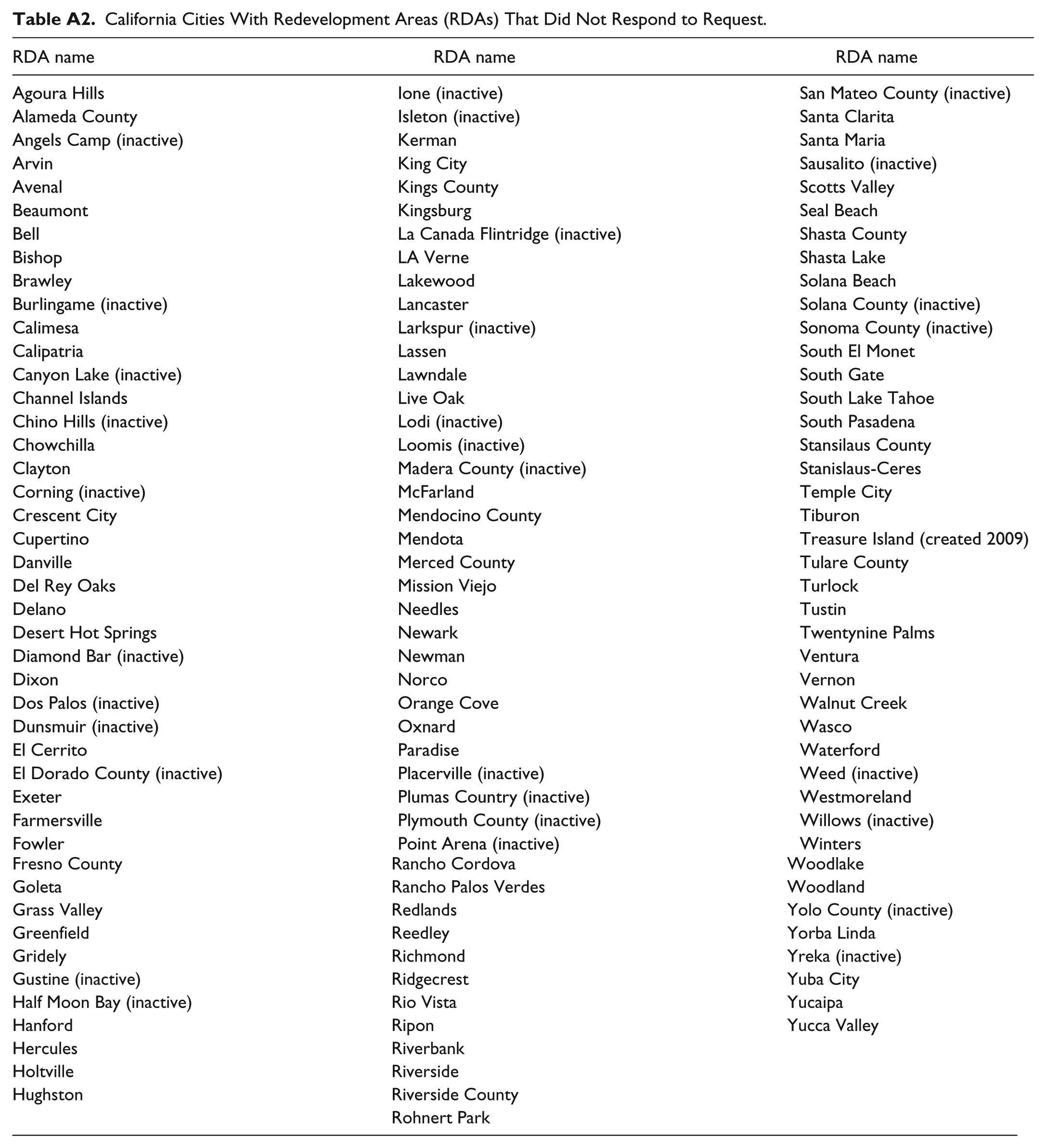
Because precise locations of California RDAs are not publicly available in any centralized source, individual cities’ RDAs were contacted to provide maps for RDA areas existing as of 2000. 13 Of the 415 RDAs from which maps were requested, 131 did not respond 14 ; however, 29 RDAs were inactive so no response was anticipated for these areas. The list of cities is shown in Appendix A. The maps were then digitized using geographic information system (GIS) software. Areas immediately adjacent to the RDA areas were also digitized. For the sake of conservatism, areas we designated as near RDAs needed to specify two conditions: They were outside of the RDA periphery (thus minimizing the chance that at one time they were an RDA) and no part of an RDA was contained in the related census tract.
Corresponding census tract numbers were then extracted from the GIS maps. Census data were then obtained for the corresponding tracts. The resultant data, based on 2000 census tract definitions, consist of census tracts that belong in California RDAs from 1990 through 2000. 15 A database of all census tracts bordering all RDA census tracts, which we call near-RDAs (NRDA), and of all other census tracts (Rest) was then created. NRDAs were defined two ways: all tracts bordering RDA tracts and each tract closest to each RDA tract (in terms of closest geographic centroid). The purpose of creating data for these last two groups of census tracts will be discussed in the next section. After RDA boundaries were digitized, every 2000 census tract was coded as to whether it fell within an RDA, 16 bordered an RDA, or did neither. This database of RDA tracts was matched to the U.S. Census Bureau data for 1980, 1990, and 2000. The census data contains detailed demographic information on the unemployment rate, poverty rate, income, vacancy rates, and so on at the census tract level. Technical details of this process are reported in Appendix B.
Business-level data are drawn from the National Establishment Time Series (NETS) database. The NETS database is a unique, establishment-specific database derived from Dun & Bradstreet, the latter of which is used commercially. This data set became available to academics in 2007. The 2009 NETS database includes an annual time series of information on over 36.5 million U.S. establishments from January 1990 to January 2010. Unlike other program-readable annual firm databases (such as Standard and Poor’s Compustat), NETS reports exact geographic locations of establishments, as well as other variables such as sales, employment, and Standard Industrial Classification Codes (SIC). A number of academic papers have included this database. 17 The overall reliability of Dun & Bradstreet data, which underlies the NETS data, is considered high because this database has been in existence for many years. Establishment addresses for this database were geocoded to provide corresponding census tract numbers, and the establishments were then tagged as belonging to RDA tracts, nearby tracts (either contiguous or closest to an RDA tract), and all other tracts. Resultant sales revenues and employment were then extracted for establishments for all such tracts.
Research Design
Research into this topic is potentially hampered by the difficulty of distinguishing the effects of RDA policies from the effects of other RDA characteristics that are unrelated to policy. By definition, these areas perform very poorly along many economic indicators. Thus, simply examining the performance of these areas along some economic indicators may be misleading.
The general research design here is to look at trends in RDA areas versus trends in areas near RDAs (a control group), while controlling for trends in previous time periods. This differences-in-differences approach 18 is discussed later. Ideally, we could compare not only RDAs and near-RDA areas to each other, but also RDAs and near-RDAs to themselves at a prior point in time. For example, it would be ideal to compare economic conditions of RDA areas before and after RDA designation. The main problem with the “before” comparisons is that California RDAs were designated at various times throughout the 1960s, 1970s, 1980s, and 1990s. 19 In fact, all but 34 of them 20 were established in the 1980s or earlier. A further data problem relates to census tract definitions. Although 1980, 1990, and 2000 tract boundaries are quite similar, boundaries before 1980 were quite different. Thus, matching pre-1980 data to 1980 and later years would be very problematic. Accordingly, our outcome variables are restricted to 1980 through 2000.
Thus, the differences-in-differences approach can only be used for RDAs established in the 1990s. However, RDAs established before the 1990s can also be examined by attempting to control for endogeneity using an instrumental variable approach. Despite the differences in the two RDA groups and analyses methods, as discussed later, very similar results were derived.
Results
Redevelopment Areas Established in the 1990s: Descriptive Statistics
As noted previously, because of census data limitations, the analysis is divided between RDAs established pre- and post-1990. In this section, data are provided on census tracts that belong to RDAs versus census tracts that are located right next to RDAs. If more than one non-RDA tract touched an RDA tract, then the closest tract (in terms of geographic centroid) was used as the matched tract. In principle, these matched tracts could be north, south, east, or west of their RDA tract counterparts. Table 1 reports the economic conditions that prevailed in these areas in 1980, 1990, and 2000 21 in terms of means. The economic condition variables for tract residents are poverty rates, unemployment rates, family income, wage and salary incomes, residential vacancy rates, and average monthly rents (for residential property). Table 1 shows that there was essentially no difference (statistically speaking) in changes in any of these variables in areas that would become RDAs versus nearby tracts in the 1980s. This suggests that the nearby tracts are reasonable comparison groups. On the other hand, there is also not much difference (statistically) for 1990s changes between the two groups (i.e., after RDA designation), suggesting that RDA designation did not have any noticeable effect.
Summary Statistics (Means) for RDAs Established in 1990s.
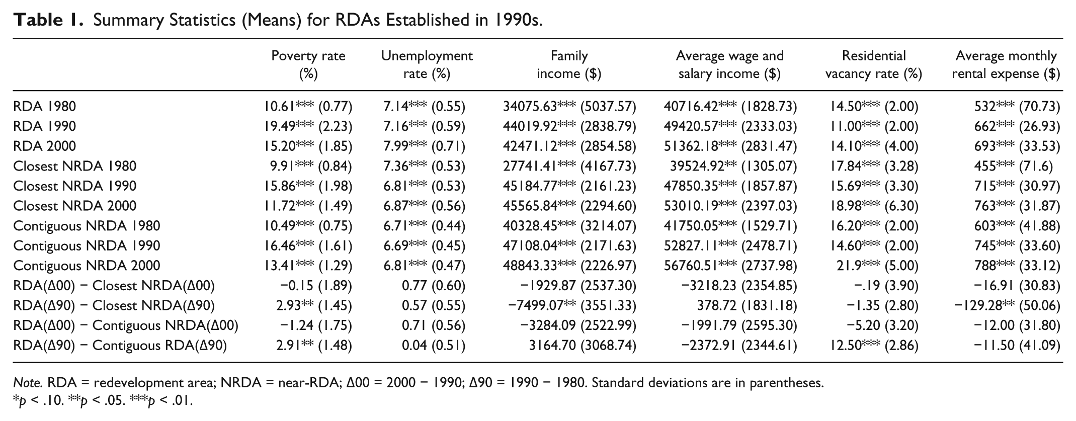
Note. RDA = redevelopment area; NRDA = near-RDA; Δ00 = 2000 − 1990; Δ90 = 1990 − 1980. Standard deviations are in parentheses.
p < .10. **p < .05. ***p < .01.
The next section investigates if the differences documented in the following tables are statistically significant, using regression analysis.
Redevelopment Areas Established in the 1990s: Statistical Tests of Significance
In this section, the econometric approach and the results of this approach are described. The effects of trends are considered by using a differences-in-differences estimation method. In contrast to a within-subjects estimate of the treatment effect (that measures the difference in an outcome after and before treatment) or a between-subjects estimate of the treatment effect (that measures the difference in an outcome between the treatment and control groups), the standard differences-in-differences estimator represents the difference between the pre–post, within-subjects differences of the treatment and control groups.
The basic premise of differences-in-differences is to examine the effect of some sort of treatment by comparing the treatment group after treatment, both with the treatment group before treatment and with some other control group. For RDAs established before 1990 (because of the census data limitations, noted above), outcomes before the treatment cannot directly be observed (i.e., periods before the RDA was established). For such pre-1990 RDAs, it is instead assumed that the “treatment” is continuously reapplied over time; that is, RDA status tends to persist because, although the area improves, it is still more blighted than other areas. In the following paragraphs, such a model is discussed in the traditional differences-in-differences approach; then it is discussed and applied in a more restrictive specification.
Assume a census tract i at any time t, where t is a census decile period. Those tracts designated as RDAs are shown below with a dummy variable RDA. The comparison group denoted NRDA 22 can be either the closest non-NRDA census tract (hereafter Model 1), all adjacent census tracts (hereafter Model 2), or all other census tracts in the state (hereafter Model 3).
Consider an outcome variable

where:

Using 2000 data as t + 1 observations, 1990 data as t observations, and 1980 data as t − 1, regression results for the above Models 1, 2, and 3 are shown in Table 2. Panel A shows that RDA poverty rates declined 4% or more relative to comparison tracts after RDA designation, but this decline was not statistically significant under Models 1 and 2. On the other hand, there was a 5.9% decline in poverty rates relative to the rest of the state (Model 3) after RDA designation, and this effect was statistically significant. Panel A also reports results for unemployment rates; here, there was no significant difference between RDAs and any comparison group after RDA designation. Panel B shows that RDAs outperformed their comparison groups with respect to family income or wage and salary incomes in only one case after RDA designation. 24 Panel C shows that RDA residential vacancy rates and residential median monthly rents were not different (in terms of statistical significance) from comparison area tracts.
Regression Results for RDAs Established in the 1990s.
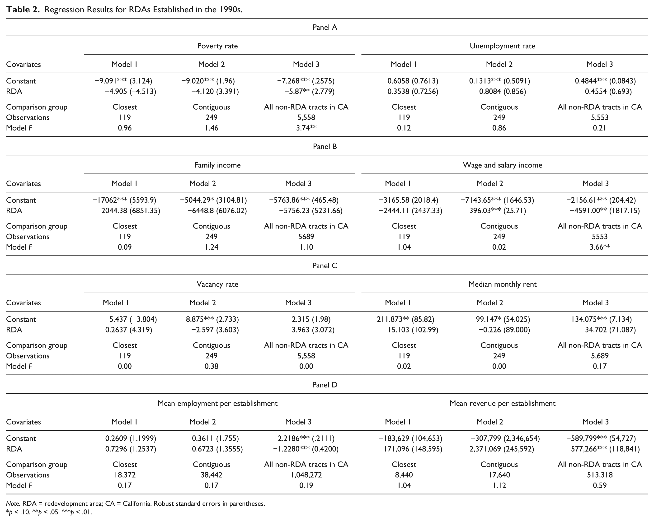
Note. RDA = redevelopment area; CA = California. Robust standard errors in parentheses.
p < .10. **p < .05. ***p < .01.
Regressions examining the effects of RDAs on business activity are shown in Panel D. Since the NETS database is not available before 1990, the research design here is slightly different. Because pre-1990 changes cannot be observed, the dependent variable is the change in sales (or employment) from 1990-2000. 25 Models 1 and 2 show that establishments in RDAs did not experience significant employment or revenue growth relative to establishments in nearby census tracts after RDA designation. Mixed results are reported for Model 3; RDA establishments actually decreased employment relative to the rest of the state, although revenues for these firms increased more than for establishments in the rest of the state. The results are essentially the same if we examine changes all the way through 2009 (the most current year in the NETS database). 26
As noted in Dye and Merriman (2000), creating a TIF (in our case, an RDA) could be because of two opposing reasons: The area is on a downward trajectory or some expected potential new development will increase property values and economic conditions. The first scenario might understate the impact of RDAs relative to other areas, whereas the second reason might overstate the RDAs impact relative to other areas. In either case, economic factors lead to a nonrandom assignment of the areas designated creating a potential endogeneity problem. Most of the prior research has either assumed such potential violations of the conditional independence assumption (CIA) were not material or controlled for them using an instrumental variable approach, fixed effects, or by using a propensity score.
To test whether the above disappointing results were because of potential endogeneity, the above regressions were rerun using an instrumental variable for the RDA dummy. 27 This is estimated from first-stage regressions where RDA is regressed on all other census data other than the dependent variable reported in any particular table. Results of these instrumental variable regressions are reported in Table 3. The results are not much different from those reported in Table 2 in terms of coefficients and statistical significance. Except for a reduction in poverty rates under Model 3, the results again show that for RDAs established in the 1990s, neither residents nor firms located in RDAs experienced any meaningful economic improvement.
Instrumental Variable (IV) Estimates of the Effects of RDAs Established in 1990s.
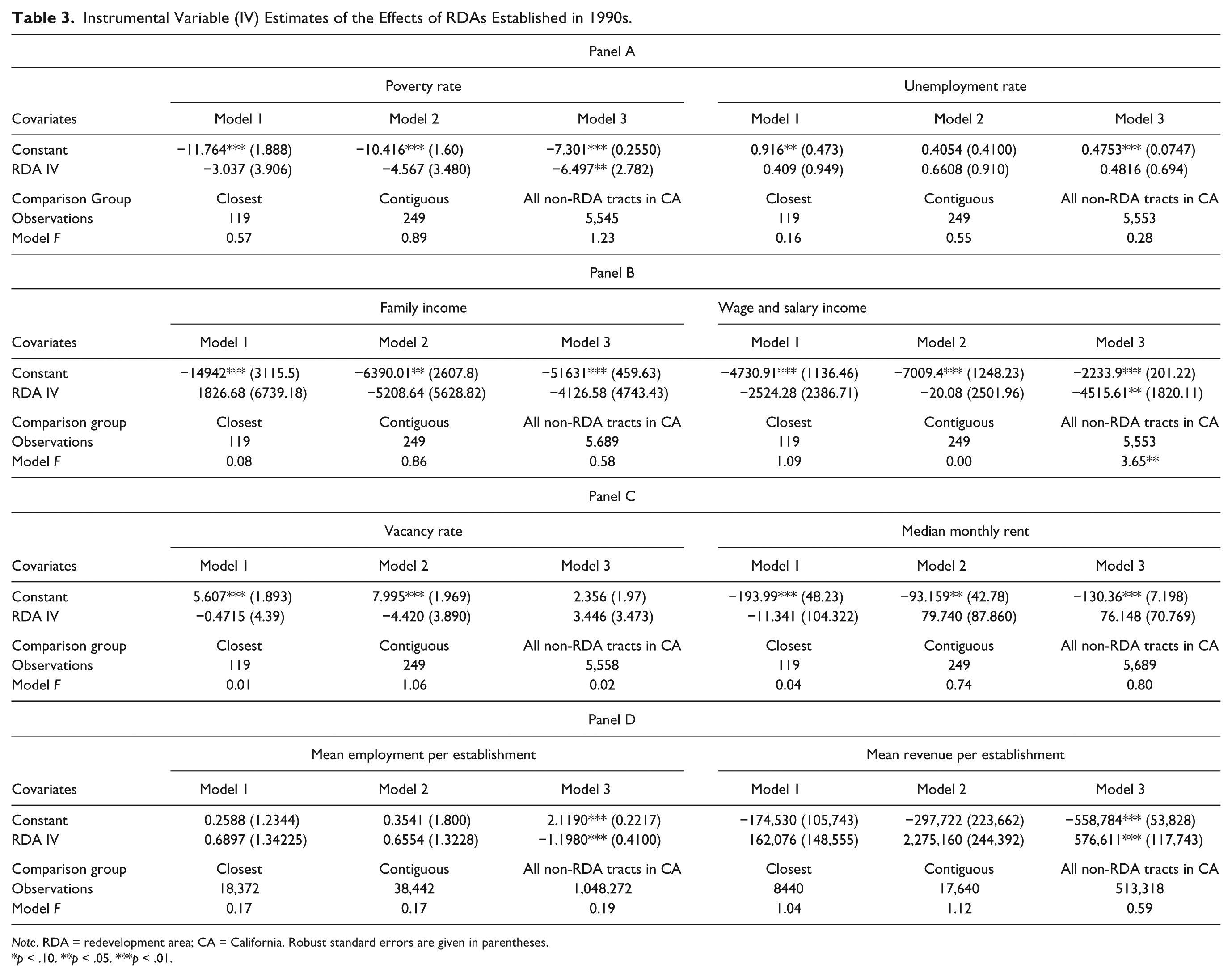
Note. RDA = redevelopment area; CA = California. Robust standard errors are given in parentheses.
p < .10. **p < .05. ***p < .01.
Redevelopment Areas Established Before the 1990s
As noted above, the vast majority of RDAs in California were established at various times in the 1950s through the 1980s. Examining this larger data set provides a larger and richer sample. On the other hand, it comes at the cost of not being able to control for pre-RDA designation trends, as in the case of 1990s RDAs. Nonetheless, if it is assumed that 1980 trends in such RDAs as well as in nearby comparison census tracts followed similar trends, a similar differences-in-differences specification can be employed. If little improvement is still observed in economic conditions in RDAs, there is some corroboration for the findings for 1990s RDAs.
Descriptive results reported in Table 4 suggest mixed results. Depending on which census tracts are used as the comparison group, RDA tracts show either some improvement, no improvement, or actually performed worse in the 1990s. Regression results for the 1990s are reported in Table 5. Poverty and unemployment rates significantly improved, but only under Model 3. Wage and salary incomes improved, but only under Model 3, and family incomes actually significantly dropped for two of the three models. Similarly, except for vacancy rates under Model 3, results were not significant for either vacancy rates or median rents. Similar weak results are reported for businesses in Panel D. Establishment employment increased by 1% (but only under one of the three models), and establishment revenues increased by approximately 145,000, but only under one model as well. As with results using establishment data reported in previous tables, the results here should be interpreted with caution because the NETS data do not start until 1990 and there is no control for pre-1990 trends.
Summary Statistics (Means) for RDAs Established Before 1990.
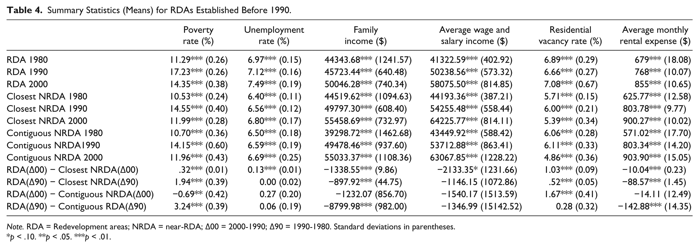
Note. RDA = Redevelopment areas; NRDA = near-RDA; Δ00 = 2000-1990; Δ90 = 1990-1980. Standard deviations in parentheses.
p < .10. **p < .05. ***p < .01.
Estimates of the Effects of RDAs Established Prior to 1990s.
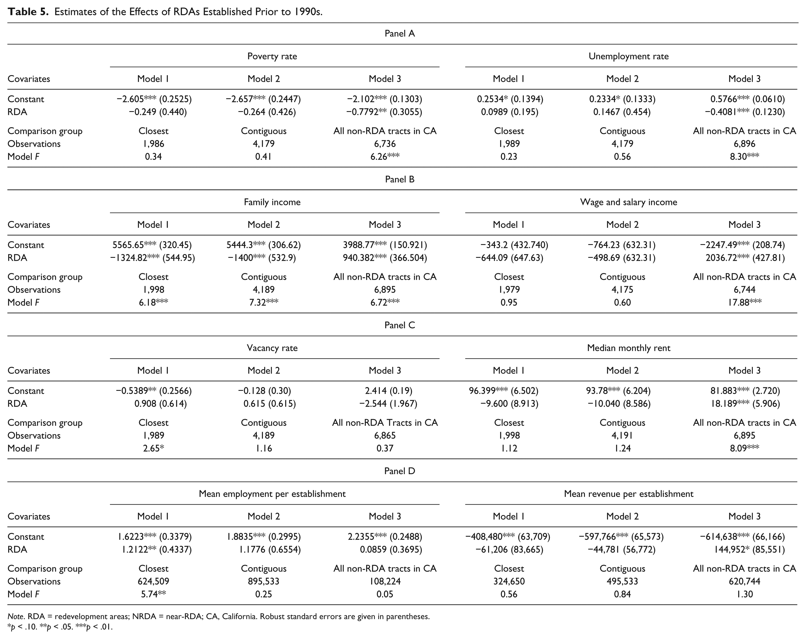
Note. RDA = redevelopment areas; NRDA = near-RDA; CA, California. Robust standard errors are given in parentheses.
p < .10. **p < .05. ***p < .01.
Table 6 reestimates the Table 5 regressions with an instrumental variable specification for the RDA variable. Results in terms of parameter estimates and statistical significance are similar to those reported in Table 6. Except for significant drops in poverty and unemployment under Model 3 and increases in wage/salary income and median rents under Model 3, results are either insignificant or show worsening conditions in RDAs for census data in the 1990s. Business data, reported in Panel D, are not much different (in terms of general coefficients and significance) from what is reported in Table 5.
Instrumental Variable (IV) Estimates of the Effects of RDAs Established Prior to the 1990s.
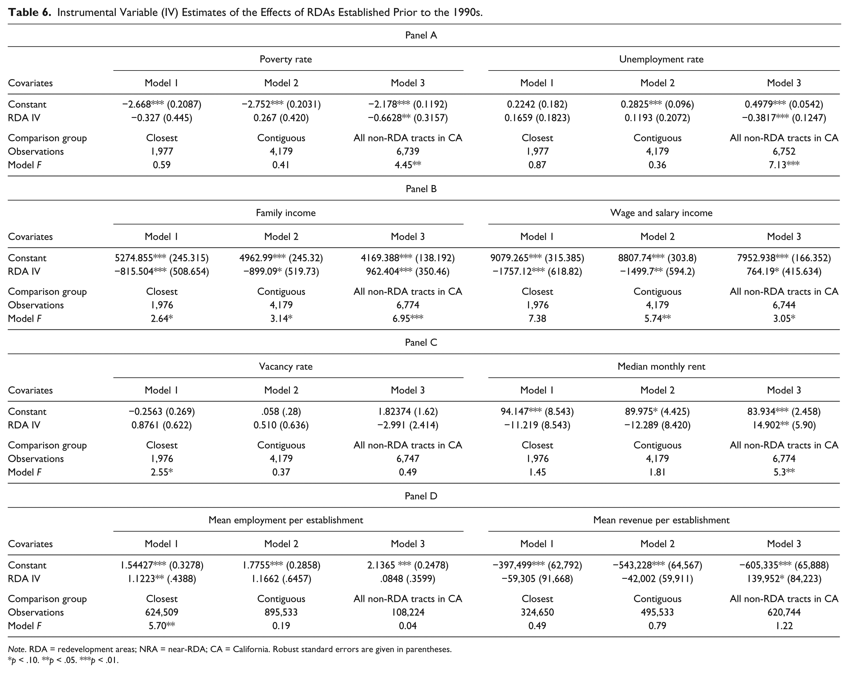
Note. RDA = redevelopment areas; NRA = near-RDA; CA = California. Robust standard errors are given in parentheses.
p < .10. **p < .05. ***p < .01.
It may be the case that various areas did not follow similar trends prior to 1990. Regressions examining only 1990-2000 changes were run (i.e., not a differences-in-differences estimate taking out pre-1990 trends) and results were qualitatively similar; RDA tracts did not significantly outperform either nearby tracts or all other tracts in the state. These results were not sensitive to inclusion of the 1980 levels of the dependent variable as a control (e.g., if 1990-2000 changes in poverty are examined, 1980 poverty levels for that tract are included as a variable) or to various specifications using an instrumental variable measure for RDA designation.
Conclusions
The economic impact of California RDAs is examined by comparing economic activity within an RDA with nearby areas. Digitized maps of hundreds of RDAs were created from paper maps then converted to census tracts and related census data from 1980 through 2000 were then analyzed. Control groups of nearby census tracts were also created. When RDAs established in the 1990s are examined, the only consistently positive impact of RDA designation was for average revenues for establishments in RDAs. When RDAs established prior to the 1990s are examined, the poverty and unemployment rates were lower in RDAs, and wage and salary incomes, family incomes, and monthly median rents were all larger in RDAs. But these results were not consistent and were obtained for just one of the three model specifications. 28
Subsequent to the program’s dismantling, the state appointed “successor entities” for each RDA. In the vast majority of cases, the cities in which the RDAs were located became successors. The new entities are responsible for the settling of existing obligations and the handling of any pretermination funds. At this point, it is difficult to assess the long-run impact that the program’s dismantling will have on local area economies and that of the state as a whole.
Although California represents a significant sample size and its RDA program is similar to TIF programs used in many other states, the results cannot necessarily be generalized to other states without performing state-specific studies.
Footnotes
Appendix A
California Cities With Redevelopment Areas (RDAs) That Did Not Respond to Request.
| RDA name | RDA name | RDA name |
|---|---|---|
| Agoura Hills | Ione (inactive) | San Mateo County (inactive) |
| Alameda County | Isleton (inactive) | Santa Clarita |
| Angels Camp (inactive) | Kerman | Santa Maria |
| Arvin | King City | Sausalito (inactive) |
| Avenal | Kings County | Scotts Valley |
| Beaumont | Kingsburg | Seal Beach |
| Bell | La Canada Flintridge (inactive) | Shasta County |
| Bishop | LA Verne | Shasta Lake |
| Brawley | Lakewood | Solana Beach |
| Burlingame (inactive) | Lancaster | Solana County (inactive) |
| Calimesa | Larkspur (inactive) | Sonoma County (inactive) |
| Calipatria | Lassen | South El Monet |
| Canyon Lake (inactive) | Lawndale | South Gate |
| Channel Islands | Live Oak | South Lake Tahoe |
| Chino Hills (inactive) | Lodi (inactive) | South Pasadena |
| Chowchilla | Loomis (inactive) | Stansilaus County |
| Clayton | Madera County (inactive) | Stanislaus-Ceres |
| Corning (inactive) | McFarland | Temple City |
| Crescent City | Mendocino County | Tiburon |
| Cupertino | Mendota | Treasure Island (created 2009) |
| Danville | Merced County | Tulare County |
| Del Rey Oaks | Mission Viejo | Turlock |
| Delano | Needles | Tustin |
| Desert Hot Springs | Newark | Twentynine Palms |
| Diamond Bar (inactive) | Newman | Ventura |
| Dixon | Norco | Vernon |
| Dos Palos (inactive) | Orange Cove | Walnut Creek |
| Dunsmuir (inactive) | Oxnard | Wasco |
| El Cerrito | Paradise | Waterford |
| El Dorado County (inactive) | Placerville (inactive) | Weed (inactive) |
| Exeter | Plumas Country (inactive) | Westmoreland |
| Farmersville | Plymouth County (inactive) | Willows (inactive) |
| Fowler | Point Arena (inactive) | Winters |
| Fresno County | Rancho Cordova | Woodlake |
| Goleta | Rancho Palos Verdes | Woodland |
| Grass Valley | Redlands | Yolo County (inactive) |
| Greenfield | Reedley | Yorba Linda |
| Gridely | Richmond | Yreka (inactive) |
| Gustine (inactive) | Ridgecrest | Yuba City |
| Half Moon Bay (inactive) | Rio Vista | Yucaipa |
| Hanford | Ripon | Yucca Valley |
| Hercules | Riverbank | |
| Holtville | Riverside | |
| Hughston | Riverside County | |
| Rohnert Park |
Appendix B
Acknowledgements
The author gratefully acknowledges the helpful suggestions of David Merriman.
Declaration of Conflicting Interests
The author(s) declared no potential conflicts of interest with respect to the research, authorship, and/or publication of this article.
Funding
The author(s) received no financial support for the research, authorship, and/or publication of this article.