The Optimal Time Decay Rates and Vanishing Limit for Three-Dimensional Incompressible Phan-Thien–Tanner and Oldroyd-B Systems in the Critical Besov Spaces
Available accessResearch articleFirst published online 2026
The Optimal Time Decay Rates and Vanishing Limit for Three-Dimensional Incompressible Phan-Thien–Tanner and Oldroyd-B Systems in the Critical Besov Spaces
In this article, we study the incompressible Phan-Thien–Tanner (PTT) and Oldroyd-B systems in . The interesting features of the Cauchy problem studied in this work are the well-posedness and large-time behavior of global solutions for the PTT and Oldroyd-B systems with or without a damping mechanism, and the relationship between these two systems in the critical Besov spaces. First, we study the well-posedness of global solutions with data having critical regularity in the case of small initial data by proving uniform estimates with respect to the parameters and . Second, we prove the optimal time decay rates of global solutions in by exploiting harmonic analysis tools, such as non-standard product estimates, various Sobolev embeddings, and interpolation inequalities. We only assume that the negative Besov norm at low frequencies of the initial data is bounded and remove the () condition, which has been required in previous works on this problem. Finally, we investigate the convergence of global solutions to the PTT system when tends to . Moreover, the specific rate of convergence is obtained in some sense.
The homogeneous flows of incompressible isothermal polymer fluids can be described by the continuity and momentum balance equations. It is universally acknowledged that polymer molecules may be extraordinarily complex objects, but there are some theories and methods to simplify and model them. In particular, the model considered in this article originates from the work in 1977 by N. Phan-Thien and R. I. Tanner in Phan-Thien and Tanner (1977), governed by
This model is developed to describe the rheological behavior of viscoelastic fluids. The unknowns are the fluid velocity, the isotropic fluid pressure, and the stress tensor, respectively. Moreover, the symmetric tensor of constraints corresponds to the rates of creation and destruction of junctions, depending on the instantaneous elastic energy of the network or, equivalently, the average extension of the network strand. Then, may be divided into two parts: the elastic part and the Newtonian part, that is,
where is the polymer contribution to the stress tensor, the positive real number is the solvent viscosity coefficient, is the elastic coefficient, and . We denote the objective derivative of the tensor by , defined as
where is the slip parameter, and . We focus on the linear Phan-Thien–Tanner (PTT) model, which is a well-studied phenomenological constitutive model for polymer fluids. It is given by
where is the relaxation time of the fluid, is the retardation time of the fluid, is the polymer viscosity, and is a parameter controlling the elongational viscosity.
We set , , and , to deduce the following linear incompressible PTT system:
where the positive real numbers and are associated with the Deborah number , which indicates the relation between the characteristic flow time and the elastic time (see, for instance, Bird et al., 1977), and the non-negative real number is related to the rates of creation and destruction of the polymeric network junctions. Here, is a given bilinear form
where the physical parameter . In particular, we call the system a co-rotational case when . For polymeric fluids, we note that the incompressible PTT system is derived from a constitutive equation, which is coupled to the incompressible Navier–Stokes equations. There is a substantial body of literature concerning interpretations and applications of the PTT system; see, for example, the works (Phan-Thien, 1978; Phan-Thien & Tanner, 1977).
It is interesting to note that system (1.1) reduces to the so-called Oldroyd-B system when . If there is neither the damping term nor the rates of creation and destruction of the polymeric network junctions, that is, , then system (1.1) reduces to the following Oldroyd-B system without a damping mechanism with the same initial data:
To the best of our knowledge, systems coupling fluids and polymers are of great interest in many sub-disciplines of applied sciences, such as mathematics, physics, biology, and chemistry, among others. In addition to the Oldroyd-B model, another famous model describing these systems is the PTT model. The PTT model attempts to describe the behavior of the complex mixture of polymers and fluid in more detail, and it poses a wide range of challenges, both in numerical computation and mathematics. It turns out that there are many numerical results for the PTT system (see Bautista et al., 2013; Garduño et al., 2016; Mu et al., 2013; Mu et al., 2012; Oliveira & Pinho, 1999). However, there are few mathematical results for the PTT system. In fact, the additional nonlinear term of the PTT system leads to some interesting phenomena that are quite different from those of the Oldroyd-B system. The first significant result was obtained by Masmoudi (2011), where he proved the global existence of weak solutions. Using the characteristic and energy methods, Y. Chen et al. showed in Chen, Luo, and Yao (2019), Chen, Luo, and Zhai (2019), Chen et al. (2023) that global strong solutions exist for the linear PTT system with or without a damping mechanism in both Sobolev spaces and the critical Besov spaces for small initial data. As for the global well-posedness result for the generalized PTT system in both Sobolev spaces and the critical Besov spaces, one may refer to Chen et al. (2021), Chen et al. (2023). We should mention in passing that the sharp time decay rates and stability of large solutions to the two-dimensional and three-dimensional PTT systems were established in Chen et al. (2022), Chen et al. (2023). Until very recently, the vanishing limit for the PTT system in Sobolev spaces was demonstrated in Chen et al. (2024).
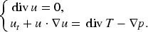
In this introductory section, we briefly explain how we consider the problems in the critical Besov spaces. In fact, the systems (1.1) and (1.2) do not have any scaling invariance, but we study the following linear mixed system:
where is the Leray projection operator and . One can easily verify that if solves system (1.3), then so does , where
Consequently, the linearized system (1.3) can be usefully employed in defining the critical space in this case. The reason for considering the well-posedness in the critical spaces has been fully explained in Chemin and Masmoudi (2001). There are many references concerning the well-posedness in the critical Besov spaces, such as Chen et al. (2010a, 2010b), Danchin (2000), Danchin (2001), Danchin and He (2016) and references therein. The hybrid Besov spaces with different indices of regularity were first established in Chen et al. (2010a).
Before getting into the heart of mathematical results, we have to introduce more notations.
Notation. For the sake of simplicity, we shall assume throughout this paper that the function space is over . The notation stands for for some irrelevant positive constant , and stands for for some irrelevant positive constant . The notation denotes . Denote by the set of tempered distributions. For any , the lower and higher oscillation parts can be expressed as
for some sufficiently large but fixed integer .
We can now state the main results and ideas of this article.
On the one hand, we are concerned with the global well-posedness and optimal time decay rates for the PTT and Oldroyd-B systems with or without a damping mechanism in the critical Besov spaces. Based on the above dissipation structure of and in system (1.3), we will show that the local well-posedness for general data and global well-posedness for small data hold for these two systems with or without a damping mechanism in the critical Besov spaces with minimal regularity. However, it does not seem possible to obtain any dissipation of when . The idea is inspired by the method applied in Chen, Luo, and Zhai (2019), Chen et al. (2021), but we then have to prove slightly more accurate estimates of the low- and high-frequency parts; see Appendices B–C for more details.
In previous papers, with the additional (, ) smallness assumption of the initial data, the following optimal time decay rate was available:
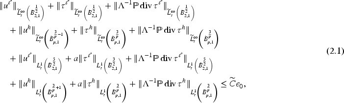
Recently, Chen et al. (2022, 2023) obtained the decay results for the PTT system under the assumptions that the initial data belong to (, ). More precisely, they obtained the decay rates of the solution and all its spatial derivatives. However, they did not verify whether the solution belongs to . Motivated by Xin and Xu (2021), we can remove this condition. For the PTT and Oldroyd-B systems with a damping mechanism (i.e., ), we can deduce the following energy estimate:
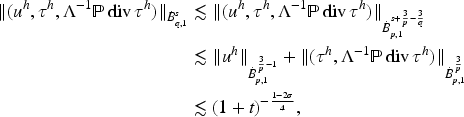
where and . Under the assumptions that the low frequencies of the initial data belong to with , we can prove that belongs to . By virtue of some elaborate use of interpolation inequalities, we find that
It is easy to deduce that
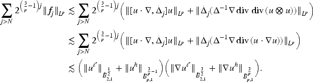
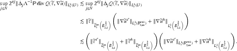
Then, with the help of non-standard product estimates and some elaborate use of Sobolev embedding inequalities, we derive the decay conclusions for the low- and high-frequency parts of with and , respectively. However, if we make additional assumptions that the initial data belong to with , we also obtain similar results. For the Oldroyd-B system without a damping mechanism (i.e., ), we additionally assume that with . We also derive similar decay conclusions of the low- and high-frequency parts of . It is worth noting that we only obtain the decay rate of instead of . As a consequence, we remove the () condition on the initial data. This is one of the innovations in our article. As a result, we obtain various decay results in many cases.
On the other hand, we are concerned with the vanishing limit for the PTT system. Both the Oldroyd-B and PTT models describe fluid-polymer systems, which are of significant interest across many sub-disciplines of applied sciences. While both are widely used, their fundamental difference lies in the nonlinear coupling: the PTT system introduces a quadratic nonlinearity through the term , creating a self-interaction mechanism absent in the Oldroyd-B system. This key distinction motivates our study, which aims to investigate the relationship between the two systems. More precisely, given some initial data, we want to obtain as much information as possible on the convergence of the solution of the PTT system as tends to . Heuristically, we want to show that the solution of the PTT system converges to that of the classical Oldroyd-B system as tends to . We then focus on the rate of convergence in the critical Besov spaces, whose norm is invariant under the scaling transformation. The main difficulties in the passage to the limit are that new nonlinear terms may arise and tends to . To address these challenging terms, we require additional regularity of the high-frequency parts of the initial data and prove uniform estimates with respect to . Then, we can pass to the limit as , and the limit obtained will be the solution to the corresponding Oldroyd-B system. It suffices to obtain the rate of convergence of the PTT system toward the corresponding Oldroyd-B system in the critical Besov spaces. We note that this is the first result studying the relationship between the PTT and Oldroyd-B systems and providing the specific convergence rate in the critical Besov spaces.
Main Results
In order to simplify the presentation, we shall assume throughout this article that . We point out that the PTT system (i.e., and ) can be used to describe more physical phenomena than the Oldroyd-B system (i.e., and ) we have seen thus far, but it is still not too cumbersome. Whether it is to prove various decay results or the vanishing limit result of the PTT system toward the corresponding Oldroyd-B system, uniform estimates with respect to and are required.
Existence Results
Our main results are based on the following two existence theorems.
Suppose that and ; the initial data , , , , with . There exists a small positive constant such that if
then system (1.1) admits a unique global solution satisfying, for any :
where is a positive constant independent of . If , then the positive constant is independent of and . If we further assume that and , there exists a positive constant (which does not need to be small) such that if
then for any :
We now verify that the conditions and are appropriate hypotheses for our problems. In the case where and , we shall see that if the initial data satisfies , then the solution of the PTT system without a damping mechanism will blow up, as shown in Chen, Luo, and Yao (2019). Therefore, the authors in Chen et al. (2023), Chen, Luo, and Zhai (2019), Chen et al. (2021) consider the global well-posedness for the PTT system without a damping mechanism under the assumptions that the initial data is a small perturbation around some particular solution. This reasoning justifies the assumption that , which is consistent with and naturally enforced by the conditions and .
We point out that for proving the vanishing limit result of the PTT system toward the corresponding Oldroyd-B system, our method requires that we additionally have the estimate (2.2).
For the Oldroyd-B system without a damping mechanism (i.e., ), we only obtain a similar existence result but for the simple case where . This is because there is no damping term for the stress tensor in system (1.2).
Suppose that . The corresponding system (1.2) admits a unique global solution with the same initial data as in Theorem 2.1 with . Moreover, the following estimate holds for any :
where is a positive constant independent of .
Decay Results
Next, we devote ourselves to investigating the optimal time decay rates of the global solutions for systems (1.1) and (1.2), respectively.
Suppose that and . Let be the global solution of system (1.1) given by Theorem 2.1. If, further, with , then for any :
and
where is a positive constant independent of . Moreover, for any and ,
for any and ,
To obtain the optimal time decay rate of the global solution in the critical Besov spaces, we require additional boundedness assumptions on the low frequencies of the initial data in , with . This is in contrast to relying on smallness assumptions of the initial data or boundedness assumptions of the solution itself. We prove that the low frequencies of the solution also lie in , provided that the low frequencies of the initial data belong to .
For the Oldroyd-B system without a damping mechanism (i.e., ), we only establish a similar result for the simple case in the following theorem.
Suppose that . Let be the global solution of system (1.2) given by Theorem 2.4. If, further, with , then for any :
and
where is a positive constant independent of . Moreover, for any and ,
for any and ,
Here, the time decay rates of the global solutions and for systems (1.1) and (1.2), respectively, are called optimal in the sense that they coincide with the time decay rates of the solutions for their linearized systems.
The difference between the decay estimates of the global solutions and for systems (1.1) and (1.2) lies in whether the optimal time decay rate of the stress tensor itself is obtained. This is due to the missing linear damping term of in system (1.2). Therefore, it follows that we can only establish the optimal time decay rate for in system (1.2).
In contrast to the definitions (1.4) and (A.1), for any , we introduce an alternative decomposition into lower and higher oscillation parts, denoted by , to replace the previous notation . The new decomposition is defined as follows:
where is a sufficiently large fixed integer. For system (1.2), we can establish similar existence and decay results for the general case . The key to the proof is Corollary B.3, so we omit the details.
Assuming that both the low- and high-frequency parts of the initial data belong to , we obtain the following theorem.
Suppose that and . Let be the global solution of system (1.1) given by Theorem 2.1. Further assuming that for some , we have for all :
where is a positive constant independent of .
For the Oldroyd-B system without a damping mechanism (i.e., ), we establish the following analogous theorem for the case .
Suppose that . Let be the global solution of system (1.2) given by Theorem 2.4. Further assuming that for some , we have for all :
where is a positive constant independent of .
In Theorems 2.5 and 2.7, we only show that the low frequencies of the solutions to systems (1.1) and (1.2) belong to , provided that the low frequencies of the initial data belong to with . A natural question is whether this regularity property extends to the solutions themselves. To ensure that the solutions to systems (1.1) and (1.2) belong to , we assume in Corollaries 2.11 and 2.12 that the initial data belong to with .
Convergence Result
We note that if , , the PTT model reduces to the Oldroyd-B model. Both the PTT and Oldroyd-B models have greater physical significance when a damping mechanism is present. We now state another convergence result as . Under the assumptions of Theorem 2.1, we establish the precise rate of convergence for the global solutions of the PTT and Oldroyd-B systems. Specifically, the following assertion holds.
Let and be the global solutions, provided by Theorem 2.1, to the PTT (with , ) and Oldroyd-B (with , ) systems, respectively. Then the following convergence result holds for all :
where is a positive constant independent of and .
The remainder of this article is organized as follows. In Section 3, we prove the global well-posedness of systems (1.1) and (1.2) under the same small perturbation assumption. In Section 4, we prove the decay results stated in Theorems 2.5, 2.7, and Corollaries 2.11, 2.12. Finally, in Section 5, we analyze the rate of convergence of the PTT system to the corresponding Oldroyd-B system. We show that this rate strongly depends on the regularity of the global solutions for both systems. In Appendices A–C, we introduce homogeneous Besov spaces, paradifferential calculus, and tools based on the Littlewood-Paley decomposition.
Global Existence
This section focuses on the proof of Theorem 2.1. First, we compare the PTT system with the Oldroyd-B system. We note that the local well-posedness of the PTT system can be proved similarly to the Oldroyd-B system, as the additional term in (1.1) contains no derivatives (see Fernández-Cara et al., 1998, Lin et al., 2005, Zhai, 2021 for details). To prove energy estimates uniformly in time for system (1.1), we define the following basic energies:
We derive the a priori estimates of , , , and . We assume that , , and .
The Estimate of
In this subsection, we derive the basic energy estimate for the low frequencies of the solution . Applying to the first equation of (1.1) and to the second, and using , we obtain
Taking the inner products of the above equations with and , respectively, and integrating by parts, we have
Thanks to the fact that , we conclude that
Integrating in time, multiplying both sides of (3.2) by , and summing the resulting inequality for , we end up with
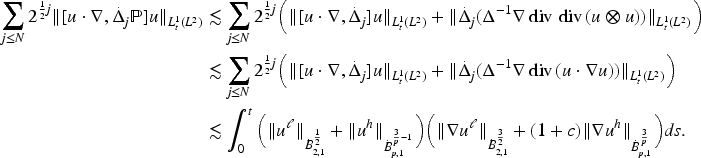
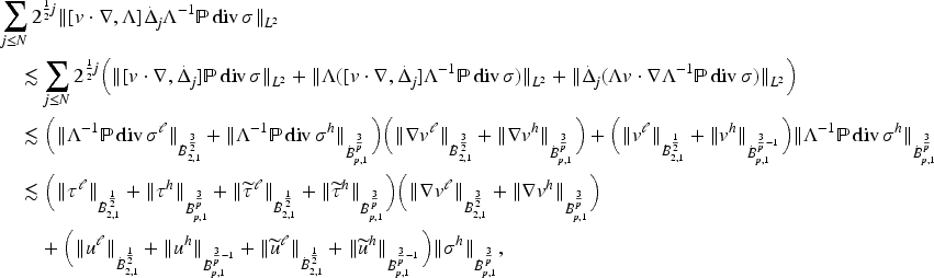
Using the commutator estimate (B.2) in Lemma B.1, the product estimate (B.19) in Lemma B.4, and the equality (C.1) in Lemma C.1, it is enough to prove that
Using the commutator estimate (B.2) in Lemma B.1 and the product estimate (B.19) in Lemma B.4 again, we have
These estimates lead to the following inequality:
where we have used the fact that . If we take , then the estimate (3.4) also holds for , and its proof is based on the last two estimates in Lemma B.6. Finally, we get
The Estimate of
In this subsection, we intend to develop a new energy estimate to provide the integrability of the low frequencies of the solution . We apply the operator to the first equation of system (1.1) and to the second one, to discover that
with
Taking the inner products of the above equations with and , respectively, then we have
Note that satisfies the following equation:
Take the inner product of the above equation with , we get that
Together with the above two estimates, we gather that
where
For any , we can choose small enough (independent of ) such that
Bernstein’s inequality asserts that
Integrating in time, multiplying both sides of the above inequality by , and summing the resulting inequality for , we obtain that
We readily have
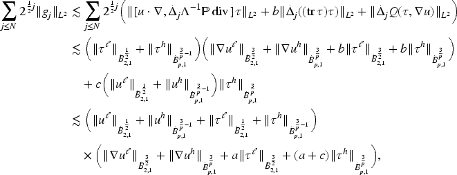
Thanks to the estimate (B.15) in Corollary B.2 and the estimate (B.19) in Lemma B.4, we verify that
where we have used the fact that . The application of the estimates (B.2) and (B.4) in Lemma B.1, the estimate (B.19) in Lemma B.4, and the equality (C.4) in Lemma C.1, gives that
Plugging the above estimates into (3.7) yields that
Integrating in time, multiplying both sides of the above inequality by , and summing the resulting inequality for , we obtain that
Hence, we have
If we take , then the estimate (3.9) also holds for . This means that
The Estimates of and
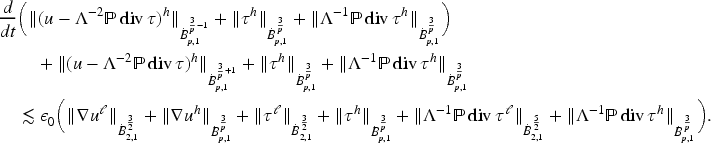
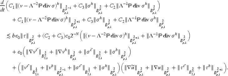
In this subsection, we are committed to deriving the energy estimate of the high frequencies of the solution . We observe that the equation for contains the linear term , where is a low-order derivative of , while the equation for depends linearly only on and itself. This structure implies that the evolution of is governed by and . In the high-frequency regime, is controlled by its dissipation and via the equation. Firstly, considering a new unknown quantity , it is obvious that
By the standard estimate, we get that
The combination of the estimates (B.3) and (B.5) in Lemma B.1, the other one (B.23) in Lemma B.4, and the equality (C.5) in Lemma C.1, ensure that
With the help of the estimate (B.3) in Lemma B.1, the other one (B.20) in Lemma B.4, and the equality (C.1) in Lemma C.1, one can obtain that
Since is a zero-order Fourier multiplier, in view of the estimate (B.16) in Corollary B.2 and the other one (B.20) in Lemma B.4, we arrive at
where we have used the fact that . Together with the above estimates, we gather that
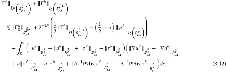
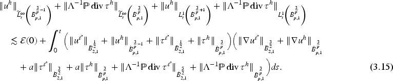
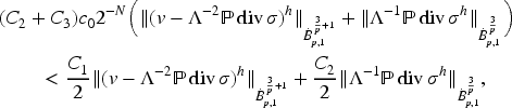
This, together with the estimate (B.5) in Lemma B.1 and the estimate (B.22) in Lemma B.4, and (3.15), yields immediately that
which implies that
If we assume, in addition, that and , then combining the above proof, we easily get that
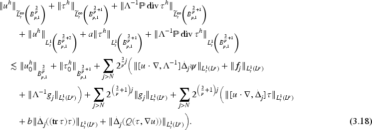
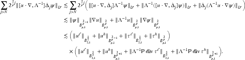
Similarly, we apply the estimate (B.3) in Lemma B.1, the other estimate (B.21) in Lemma B.4 and the equality (C.5) in Lemma C.1 to discover that
And by virtue of the estimate (B.5) in Lemma B.1 and the other one (B.21) in Lemma B.4, we find that
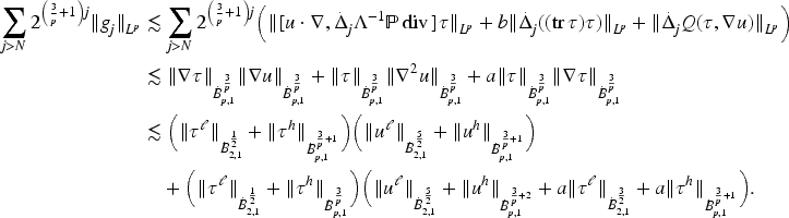
and
Using the estimate (B.5) in Lemma B.1 and the other estimate (B.21) in Lemma B.4 again, we have
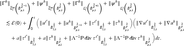
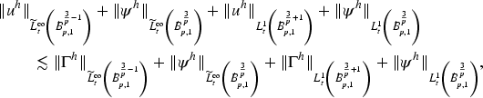
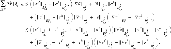
Finally, together with these estimates implies that
The Proof of Theorem 2.1
As a final step, we need to combine the estimates for , and to prove Theorem 2.1. Therefore, we deduce that for any ,
Due to the local existence theory, there exists a positive time such that
where is a positive constant independent of . If we take , from the estimates (3.4), (3.9) and (3.16) with , then we can assume that is a positive constant independent of and . Let be the largest possible time of existence of the solution with (3.21) holds. By virtue of total energy (3.20) and the smallness assumption on the initial data, we get that
Using the standard continuity argument, we can show that , provided that is small enough. Moreover, if we assume that and , from the estimate for , we find that
Then, we have
provided that is small enough. The proof of Theorem 2.1 is therefore complete.
The Proof of Theorem 2.4
If , then the proof of Theorem 2.4 is very similar to that of the previous one. Let , the idea is to take advantage of the last two estimates (B.27) and (B.28) in Lemma B.6 instead of the estimates (B.2) and (B.4) in Lemma B.1 (i.e., ). Obviously, it suffices to show that
We then infer that
Under the smallness assumption on the initial data, we can conclude that the solution exists on , whence we complete the proof of Theorem 2.4 immediately.
Large-Time Behavior
In this section, we study the precise large-time behavior of the solutions to systems (1.1) and (1.2), as given by Theorems 2.1 and 2.4, respectively. Specifically, we prove Theorems 2.5, 2.7, and Corollaries 2.11, 2.12. To this end, we employ harmonic analysis tools, including non-standard product estimates, Sobolev embeddings, and interpolation inequalities. We derive the optimal time decay rates for the solutions and to systems (1.1) and (1.2), respectively.
The Proof of Theorem 2.5
Let’s start by proving Theorem 2.5. For simplicity, we shall prove this theorem only in the case where . From the above section, we deduce from the estimate (3.4) that
provided that is small enough, and we have used the fact that
Next, we claim that
The proof of the claim (4.2) will be given in the end of this subsection. Yet by virtue of Lemma A.3 and the estimate (4.2), for any , we have
and
where we have used the fact that , which have been proven in Theorem 2.1. We also point out, for any , that
We substitute the above estimates (4.3)–(4.5) into (4.1), and choose , there then exists a positive constant such that
where
It is obvious that
For any and , we deduce that
where . Since , we have
For any and , it is easy to check that
which implies that
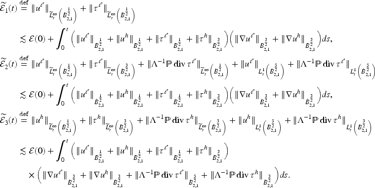
Finally, there is the claim (4.2) left to prove. In view of the estimate (3.3), we also get that
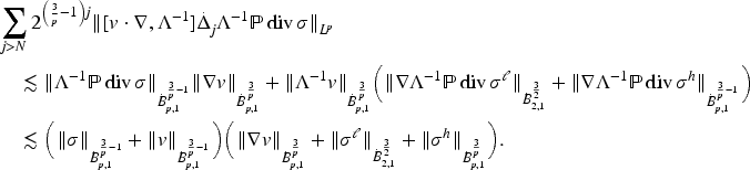
The application of the estimate (B.1) in Lemma B.1, the estimate (B.25) in Lemma B.5, and the equality (C.1) in Lemma C.1 gives that
With the help of the estimate (B.1) in Lemma B.1, we find that
We apply the estimate (B.24) in Lemma B.5, to discover that
and
Substituting the above estimates into (4.7), one can obtain that
where we have used the estimate (2.1). By choosing small enough, we can now conclude that the claim (4.2) holds. The proof is therefore complete.
The Proof of Theorem 2.7.
In this subsection, we will give the proof of Theorem 2.7. Since there is no damping term about in system (1.2), the proof of Theorem 2.7 is different from that of Theorem 2.5. For system (1.2), we first claim that
The proof of the claim (4.8) will be given in the end of this subsection. Let , the idea is to take advantage of the last two estimates (B.27) and (B.28) in Lemma B.6 instead of the estimates (B.2) and (B.4) in Lemma B.1 (i.e., ). Using the estimate (2.3), we deduce from the estimates (3.8) and (3.15) with that
and
Along the similar line as the estimate (4.6), we can get that
where . Similarly, for any and , we also have
and for any and ,
Due to , it is not hard to check that
In order to complete the proof of Theorem 2.7, we need to prove the claim (4.8). Along the similar line as the estimates (3.3) and (3.7), we find that
We apply the estimate (B.25) in Lemma B.5, the estimate (B.26) in Lemma B.6 and the equality (C.1) in Lemma C.1, to find that
The application of the estimate (B.26) in Lemma B.6 yields that
By virtue of the estimate (B.29) in Lemma B.7, we have
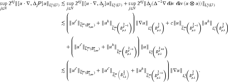
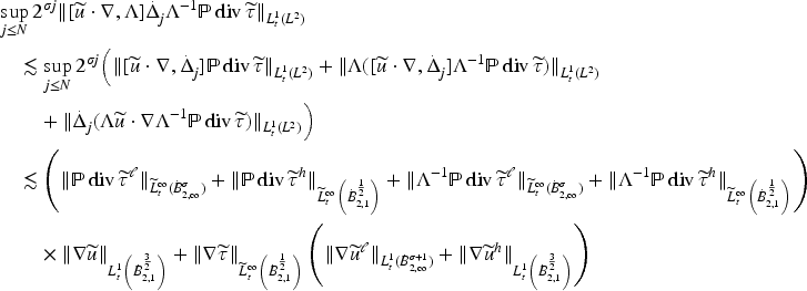
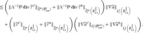
We deduce from the estimate (B.26) in Lemma B.6, the estimates (B.29) and (B.30) in Lemma B.7, and the equality (C.3) in Lemma C.1 that
In view of the estimate (B.26) in Lemma B.6, the estimate (B.29) in Lemma B.7, and the equality (C.4) in Lemma C.1, we arrive at
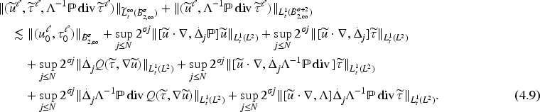
Substituting these estimates into (4.9), we find that
where we have used the estimate (2.3). By choosing small enough, we get the claim (4.8) immediately. As a consequence, the proof of Theorem 2.7 has been completed.
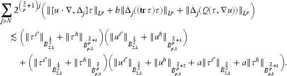
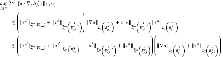
We apply the estimate (B.31) in Lemma B.8, the estimate (B.33) in Lemma B.9 and the equality (C.1) in Lemma C.1, to obtain that
The application of the estimate (B.31) in Lemma B.8 gives that
By virtue of the estimate (B.32) in Lemma B.9, we have
Substituting these estimates into (4.10), we find that
which together with the energy estimate (2.3), and by using the fact that is small enough, we finish the proof of Corollary 2.12.
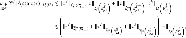
Along the similar lines, for the system (1.1), we need to treat the extra nonlinear term , that is,
Similarly, we have
which together with the energy estimate (2.1), by using the fact that is small enough, we complete the proof of Corollary 2.11.
Convergence Rate of the PTT System to the Oldroyd-B System
In Section 3, we established the existence of global solutions and for the PTT system (with , ) and the Oldroyd-B system (with , ), respectively. A natural question is whether converges to as , and if so, what is the convergence rate. This section addresses this question, and our goal is to prove Theorem 2.14. More precisely, we study the rate of convergence of the global solution for the PTT system to the global solution for the Oldroyd-B system as .
Let and be two global solutions of the PTT system (with , ) and the corresponding Oldroyd-B system (with , ) given by Theorem 2.1, respectively. In order to show that these two global solutions coincide, we shall give the uniform estimate for . For notational simplicity, we set . We shall consider the following error system satisfied by :
The proof of Theorem 2.14 will be based on Theorem 2.1, and the key of the proof is to deal with the nonlinear term . We broaden our analysis in Section 3 to cover the new system (5.1). Applying the operator to the first equation of system (5.1) and to the second one, yields that
where
It is easy to check that
and
Now following the similar argument used in Subsection 3.1, we conclude that
Applying the operator to the first equation of system (5.1) and to the second one, gives that
where
After a few calculations, we get that
and
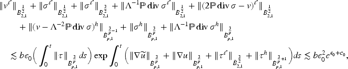
Following the similar argument used in Subsection 3.2, we have
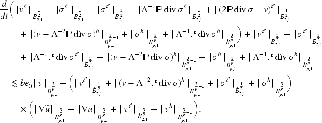
Motivated by the auxiliary variable , we estimate the combination in an analogous way. We mimic as much as possible the analysis from Subsection 3.3, then show that
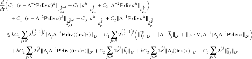
by choosing some positive constants . The estimate (B.5) in Lemma B.1 leads us to get that
In view of the estimate (B.3) in Lemma B.1, the other estimate (B.23) in Lemma B.4 and the equality (C.5) in Lemma C.1, we find that
With the help of the estimate (B.3) in Lemma B.1, the estimate (B.20) in Lemma B.4, and the equality (C.1) in Lemma C.1, one can obtain that
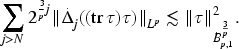
It then follows from the estimate (B.5) in Lemma B.1, the estimates (B.20) and (B.22) in Lemma B.4, and the equality (C.3) in Lemma C.1 that
This implies that
This leads us to get that,
where we have used the fact that
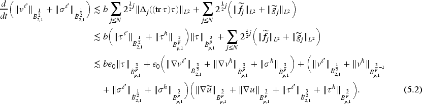
provided that and large enough. We point out that here, the smallness assumption on is not needed. Thus, from (5.2)–(5.4), we deduce that
To prove the above inequality it suffices to use the fact that is sufficiently small. The Gronwall lemma ensures that, for all ,
which leads to
The proof of Theorem 2.14 is therefore complete.
Footnotes
ORCID iDs
Yuhui Chen
Minling Li
Zheng-an Yao
Funding
The authors disclosed receipt of the following financial support for the research, authorship, and/or publication of this article: Yuhui Chen is supported by National Key R&D Program of China (Grant No. 2023YFA1010300) and Shenzhen Science and Technology Program (Grant No. JCYJ20240813151513017). Minling Li is supported by Postdoctoral Fellowship Program of CPSF (Grant No. GZB20240024) and China Postdoctoral Science Foundation (Grant No. 2024M760057 and 2025T180840).
Competing Interest
The authors declared no potential conflicts of interest with respect to the research, authorship, and/or publication of this article.
Data Availability
Data sharing not applicable to this article as no datasets were generated or analyzed during the current study.
Appendix A. Homogeneous Besov Spaces
In this section, we introduce the definition of homogeneous Besov spaces (see Bahouri et al., 2011 for more details). The homogeneous Littlewood-Paley decomposition relies upon a dyadic partition of unity. Let be an annulus There exists a radial function , belonging to , valued in the interval , and such that
Defining
The homogeneous dyadic blocks are defined by
the homogeneous low-frequency cut-off operators are defined by
We denote by the space of tempered distributions such that
Let be in , we have the following formal homogeneous Littlewood-Paley decomposition:
Furthermore, the above dyadic decomposition has nice properties of quasi-orthogonality. With our choice of , we have
Next, we introduce the Bernstein’s inequality and an interpolation inequality, which will be frequently used in this article.
In order to study the way the product acts on homogeneous Besov spaces, we shall use the following homogeneous Bony’s decomposition.
Obviously, we do not obtain an estimate in a space of type since the time integration has been performed before the summation. This naturally leads to the following definition.
Let , , and , we set
Noticing the Minkowski inequality yields if , if .
Appendix B. Some Useful Lemmas
We prove several key lemmas in this section, which will be used in the proofs of our main theorems. The first lemma concerns commutator estimates.
Following the same approach as in the proof of Lemma B.1, we derive the following two corollaries.
The following lemma concerns product estimates in Besov spaces, which are crucial for analyzing the bilinear terms in systems (1.1) and (1.2).
In Theorem 2.5, we prove that the low frequencies of the solutions lie in , provided that the low frequencies of the initial data belong to . To this end, we use the following lemma to handle the nonlinear terms.
When proving Theorems 2.4 and 2.7, handling the nonlinear terms is challenging due to the absence of the damping term for . To address this issue, we focus on the simpler case . The proof relies on the following two key lemmas. The first lemma focuses on commutator estimates.
The following lemma concerns product estimates.
For the general case , we assume in Theorems 2.11 and 2.12 that both the low- and high-frequency parts of the initial data belong to . To address this, we prove the following two key lemmas for handling the commutator and nonlinear product terms. This allows us to prove that the solutions lie in .
Appendix C. Some Useful Calculations
In this section, we perform some elementary calculations, which will be useful for handling commutators in the proofs of our main theorems.
References
1.
BahouriH.CheminJ.-Y.DanchinR. (2011). Fourier analysis and nonlinear partial differential equations (Vol. 343). Grundlehren der Mathematischen Wissenschaften, Springer.
2.
BarrettJ.LuY.SüliE. (2017). Existence of large-data finite-energy global weak solutions to a compressible Oldroyd-B model. Communications in Mathematical Sciences, 15, 1265–1323.
3.
BarrettJ.SüliE. (2011). Existence and equilibration of global weak solutions to kinetic models for dilute polymers I: Finitely extensible nonlinear bead-spring chains. Mathematical Models & Methods in Applied Sciences, 21, 211–1289.
4.
BarrettJ.SüliE. (2012). Existence and equilibration of global weak solutions to kinetic models for dilute polymers II: Hookean-type bead-spring chains. Mathematical Models & Methods in Applied Sciences, 22, 1150024.
5.
BautistaO.SánchezS.ArcosJ. C.MéndezF. (2013). Lubrication theory for electroosmotic flow in a slit microchannel with the Phan-Thien and Tanner model. Journal of Fluid Mechanics, 722, 496–532.
CheminJ.-Y.MasmoudiN. (2001). About lifespan of regular solutions of equations related to viscoelastic fluids. SIAM Journal on Mathematical Analysis, 33, 84–112.
8.
ChenQ.HaoX. (2019). Global well-posedness in the critical Besov spaces for the incompressible Oldroyd-B model without damping mechanism. Journal of Mathematical Fluid Mechanics, 21, 42.
9.
ChenY.LiM.YaoQ.YaoZ. (2021). Global well-posedness for the three-dimensional generalized Phan-Thien–Tanner model in critical Besov spaces. Journal of Mathematical Fluid Mechanics, 23, 55.
10.
ChenY.LiM.YaoQ.YaoZ. (2022). The sharp time decay rates and stability of large solutions to the two-dimensional Phan-Thien–Tanner system with magnetic field. Asymptotic Analysis, 129, 451–484.
11.
ChenY.LiM.YaoQ.YaoZ. (2023a). Sharp rates of decay and global-in-time stability of large solutions to the three-dimensional incompressible Phan-Thien–Tanner system of polymeric flows. SIAM Journal on Mathematical Analysis, 55, 4537–4569.
12.
ChenY.LiM.YaoQ.YaoZ. (2023b). Global well-posedness and optimal time decay rates for the generalized Phan-Thien–Tanner model in . Acta Mathematica Scientia. Series B. English Edition, 43, 1301–1322.
13.
ChenY.LiM.YaoQ.YaoZ. (2024). The vanishing limit for the three-dimensional incompressible Phan-Thien–Tanner system. Proceedings of the Royal Society of Edinburgh Section A: Mathematics, 154, 673–698.
14.
ChenY.LuoW.YaoZ. (2019). Blow up and global existence for the periodic Phan-Thein–Tanner model. Journal of Differential Equations, 267, 6758–6782.
15.
ChenY.LuoW.YaoZ. (2023). Global existence and optimal time decay rates for the three-dimensional incompressible Phan-Thien–Tanner model. Analysis and Applications, 21, 931–958.
16.
ChenY.LuoW.ZhaiX. (2019). Global well-posedness for the Phan-Thein–Tanner model in critical Besov spaces without damping. Journal of Mathematical Physics, 60, 061503.
17.
ChenQ.MiaoC.ZhangZ. (2010a). Global well-posedness for compressible Navier–Stokes equations with highly oscillating initial velocity. Communications on Pure and Applied Mathematics, 63, 1173–1224.
18.
ChenQ.MiaoC.ZhangZ. (2010b). Well-posedness in critical spaces for the compressible Navier–Stokes equations with density dependent viscosities. Revista Matemática Iberoamericana, 26, 915–946.
19.
DanchinR. (2000). Global existence in critical spaces for compressible Navier–Stokes equations. Inventiones Mathematicae, 141, 579–614.
20.
DanchinR. (2001). Global existence in critical spaces for flows of compressible viscous and heat-conductive gases. Archive for Rational Mechanics and Analysis, 160, 1–39.
21.
DanchinR.HeL. (2016). The incompressible limit in type critical spaces. Mathematische Annalen, 366, 1365–1402.
22.
FangD.ZiR. (2016). Global solutions to the Oldroyd-B model with a class of large initial data. SIAM Journal on Mathematical Analysis, 48, 1054–1084.
23.
FengZ.ZhuC.ZiR. (2017). Blow-up criterion for the incompressible viscoelastic flows. Journal of Functional Analysis, 272, 3742–3762.
24.
Fernández-CaraE.GuillénF.OrtegaR. R. (1998). Some theoretical results concerning non-Newtonian fluids of the Oldroyd kind. Annali della Scuola Normale Superiore di Pisa - Classe di Scienze, 26, 1–29.
25.
GarduñoI.Tamaddon-JahromiH.WaltersK.WebsterM. (2016). The interpretation of a long-standing rheological flow problem using computational rheology and a PTT constitutive model. Journal of Non-Newtonian Fluid Mechanics, 233, 27–36.
26.
GuillopéC.SautJ.-C. (1990a). Existence results for the flow of viscoelastic fluids with a differential constitutive law. Nonlinear Analysis, 15, 849–869.
27.
GuillopéC.SautJ.-C. (1990b). Global existence and one-dimensional nonlinear stability of shearing motions of viscoelastic fluids of Oldroyd type. RAIRO. Modélisation Mathématique et Analyse Numérique , 24, 369–401.
28.
HeL.XuL. (2010). Global well-posedness for viscoelastic fluid system in bounded domains. SIAM Journal on Mathematical Analysis, 42, 2610–2625.
29.
HieberM.WenH.ZiR. (2019). Optimal decay rates for solutions to the incompressible Oldroyd-B model in . Nonlinearity, 32, 833–852.
30.
HuX.WangD. (2012). Strong solutions to the three-dimensional compressible viscoelastic fluids. Journal of Differential Equations, 252, 4027–4067.
31.
HuX.WuG. (2013). Global existence and optimal decay rates for three-dimensional compressible viscoelastic flows. SIAM Journal on Mathematical Analysis, 45, 2815–2833.
32.
HuangJ.WangY.WenH.ZiR. (2022). Optimal time-decay estimates for an Oldroyd-B model with zero viscosity. Journal of Differential Equations, 306, 456–491.
33.
JiangF.JiangS. (2021). Strong solutions of the equations for viscoelastic fluids in some classes of large data. Journal of Differential Equations, 282, 148–183.
34.
LeiZ.LiuC.ZhouY. (2008). Global solutions for incompressible viscoelastic fluids. Archive for Rational Mechanics and Analysis, 188, 371–398.
35.
LeiZ.MasmoudiN.ZhouY. (2010). Remarks on the blowup criteria for Oldroyd models. Journal of Differential Equations , 248, 328–341.
36.
LeiZ.ZhouY. (2005). Global existence of classical solutions for the two-dimensional Oldroyd model via the incompressible limit. SIAM Journal on Mathematical Analysis, 37, 797–814.
37.
LinF.LiuC.ZhangP. (2005). On hydrodynamics of viscoelastic fluids. Communications on Pure and Applied Mathematics, 58, 1437–1471.
38.
LinH.WeiY.WuJ. (2022). Global well-posedness and time decay for 2D Oldroyd-B-type fluids in periodic domains with dissipation in the velocity equation only. Nonlinear Analysis. Real World Applications, 66, 103513.
39.
LinF.ZhangP. (2008). On the initial-boundary value problem of the incompressible viscoelastic fluid system. Communications on Pure and Applied Mathematics, 61, 539–558.
40.
LionsP.MasmoudiN. (2000). Global solutions for some Oldroyd models of non-Newtonian flows. Chinese Annals of Mathematics, Series B , 21, 131–146.
41.
LiuS.LuY.WenH. (2021). On the Cauchy problem for a compressible Oldroyd-B model without stress diffusion. SIAM Journal on Mathematical Analysis, 53, 6216–6242.
42.
LiuS.WangW.WenH. (2023). The Cauchy problem for an inviscid Oldroyd-B model in three dimensions: Global well posedness and optimal decay rates. Proceedings of the Royal Society of Edinburgh Section A: Mathematics , 153, 441–490.
43.
LuY.PokornýM. (2020). Global existence of large data weak solutions for a simplified compressible Oldroyd-B model without stress diffusion. Analysis in Theory and Applications, 36, 348–372.
44.
LuY.ZhangZ. (2018). Relative entropy, weak-strong uniqueness, and conditional regularity for a compressible Oldroyd-B model. SIAM Journal on Mathematical Analysis, 50, 557–590.
45.
MasmoudiN. (2011). Global existence of weak solutions to macroscopic models of polymeric flows. Journal de Mathematiques Pures et Appliquees, 96, 502–520.
46.
MuY.ZhaoG.ChenA.WuX. (2013). Modeling and simulation of three-dimensional extrusion swelling of viscoelastic fluids with PTT, Giesekus and FENE-P constitutive models. International Journal for Numerical Methods in Fluids, 72, 846–863.
47.
MuY.ZhaoG.WuX.ZhaiJ. (2012). Modeling and simulation of three-dimensional planar contraction flow of viscoelastic fluids with PTT, Giesekus and FENE-P constitutive models. Applied Mathematics and Computation, 218, 8429–8443.
48.
OldroydJ. (1958). Non-Newtonian effects in steady motion of some idealized elastico-viscous liquids. Proceedings of the Royal Society A: Mathematical, Physical and Engineering Sciences, 245, 278–297.
49.
OliveiraP.PinhoF. (1999). Analytical solution for fully developed channel and pipe flow of Phan-Thien–Tanner fluids. Journal of Fluid Mechanics, 387, 271–280.
50.
Phan-ThienN. (1978). A nonlinear network viscoelastic model. Journal of Rheology, 22, 259–283.
51.
Phan-ThienN.TannerR. (1977). A new constitutive equation derived from network theory. Journal of Non-Newtonian Fluid Mechanics, 2, 353–365.
52.
QianJ.ZhangZ. (2010). Global well-posedness for compressible viscoelastic fluids near equilibrium. Archive for Rational Mechanics and Analysis, 198, 835–868.
53.
SunY.ZhangZ. (2011). Global well-posedness for the 2D micro-macro models in the bounded domain. Communications in Mathematical Physics, 303, 361–383.
54.
WangW.WenH. (2020). The Cauchy problem for an Oldroyd-B model in three dimensions. Mathematical Models & Methods in Applied Sciences, 30, 139–179.
55.
XinZ.XuJ. (2021). Optimal decay for the compressible Navier–Stokes equations without additional smallness assumptions. Journal of Differential Equations, 274, 543–575.
56.
ZhaiX. (2021). Global solutions to the -dimensional incompressible Oldroyd-B model without damping mechanism. Journal of Mathematical Physics, 62, 021503.
57.
ZhangT.FangD. (2012). Global existence of strong solution for equations related to the incompressible viscoelastic fluids in the critical framework. SIAM Journal on Mathematical Analysis, 44, 2266–2288.
58.
ZhouZ.ZhuC.ZiR. (2018). Global well-posedness and decay rates for the three dimensional compressible Oldroyd-B model. Journal of Differential Equations, 265, 1259–1278.
59.
ZhuY. (2018). Global small solutions of 3D incompressible Oldroyd-B model without damping mechanism. Journal of Functional Analysis, 274, 2039–2060.
60.
ZiR.FangD.ZhangT. (2014). Global solution to the incompressible Oldroyd-B model in the critical framework: The case of the non-small coupling parameters. Archive for Rational Mechanics and Analysis, 213, 651–687.