
Abstract
Using representative cross-sections from 166 nations (more than 1.7 million respondents), we examined differences in three measures of subjective well-being over the life span. Globally, and in the individual regions of the world, we found only very small differences in life satisfaction and negative affect. By contrast, decreases in positive affect were larger. We then examined four important predictors of subjective well-being and how their associations changed: marriage, employment, prosociality, and life meaning. These predictors were typically associated with higher subjective well-being over the life span in every world region. Marriage showed only very small associations for the three outcomes, whereas employment had larger effects that peaked around age 50 years. Prosociality had practically significant associations only with positive affect, and life meaning had strong, consistent associations with all subjective-well-being measures across regions and ages. These findings enhance our understanding of subjective-well-being patterns and what matters for subjective well-being across the life span.
A pervasive concern among many people across the world is that growing older and reaching senior status means leaving their best days behind. However, a fair bit of longitudinal and cross-sectional research has shown that levels of happiness remain relatively stable across the life span (Lucas & Gohm, 2000), at least until one comes close to death (Gerstorf et al., 2008). However, prior research is not all consistent (for a review, see Ulloa, Moller, & Sousa-Poza, 2013). One often-cited finding is of a U-shaped curve over the life span that has its lowest point in middle age. This trend has been replicated in many different data sets across many world regions (Blanchflower & Oswald, 2008, 2018; Graham & Pozuelo, 2017). However, the topic is unresolved because these past studies also had limitations.
The first limitation is that most of the researchers who conducted these studies based their conclusions only on life satisfaction, which is a cognitive assessment of happiness (Diener, 1984), but the subjective-well-being construct (the scientific concept for “happiness”) traditionally has two additional measures, positive affect and negative affect (Diener, 1984). Many scholars argue that it is necessary to examine all three in order to draw conclusions about subjective well-being (Diener & Biswas-Diener, 2002; Lucas, Diener, & Suh, 1996). Second, it is possible that the U-shaped (or other) curve exists but that it is so small that it is not practically meaningful. In other words, just because differences across age are statistically significant, that does not mean that these differences have practical significance (Fritz, Morris, & Richler, 2012). Researchers in past studies have generally not taken effect size into account, but effect size is necessary to examine this topic. Finally, many researchers have based their conclusions on data from just one or several nations rather than sampling from a large share of the entire world (cf. Graham & Pozuelo, 2017; Margolis & Myrskylä, 2013). This makes it difficult to compare findings across various world regions and to develop generalized conclusions about the shape of happiness across age.
In the current study, we sought to address these past limitations. We did so by examining how subjective well-being differs across the life span in the Gallup World Poll, a representative cross-section from more than 160 countries and 1.7 million respondents. We examined how three measures of subjective well-being (life satisfaction, positive affect, negative affect) differed across age in 10 sociocultural regions of the world while looking at effect size and factoring in practical significance in our scientific conclusions.
Changing Priorities Across the Life Span
Although how subjective well-being differs across age is important, we also asked a secondary research question: How do its associations with predictors change? At different points in life, priorities and life circumstances change, and thus we can expect that the predictors of happiness may also change (Oishi, Diener, Suh, & Lucas, 1999). For instance, some research suggests that intimacy and romantic relationships tend to be highly valued in young adulthood (Sheldon & Kasser, 2001), that prosociality and work productivity may become more important in middle age, and that life meaning might be more prioritized among older individuals (Huta & Zuroff, 2007; Lelkes, 2008; Margolis & Myrskylä, 2013). Given that increasing numbers of people are living longer, it is critical to understand the factors that shape their well-being at different stages in life and how these may be influenced by sociocultural factors. Therefore, we asked the following questions: How do the associations between happiness and predictors vary across the life span? Are there any predictors that are universal across ages or regions of the world?
We chose to focus on four predictors: marriage, employment, prosociality, and life meaning. These four were chosen because of their psychological significance. Work and romantic partnerships are two of the most important domains of human life, and prosociality and life meaning are two variables that strongly relate to how one relates to others and to the world. By analyzing these predictors within the Gallup World Poll, using three measures of subjective well-being, and taking into account practical significance, we sought to gain a better understanding of their generalizability across the life span and around the world.
Method
Sample
Gallup surveyed 1,709,734 individuals (age range = 15–99 years, M = 40.87, SD = 17.40) from 166 countries across the years 2005 to 2016 (Gallup, 2016). In countries where telephone penetration is 80% or higher, this was achieved through random-digit-dialing telephone surveys. In less developed nations, where telephone penetration is less than 80%, surveys were conducted by in-person interviews; residences were selected from a geographical area frame. Primary sampling units were stratified by population size or geography, and random route procedures were used to select households. At least three attempts were made to reach a person in each selected household (unless they refused sooner). Respondents within households were selected on the basis of either the latest birthday or the Kish grid method. Up to three contacts per household were used at different times of day. A few regions of certain countries were not sampled because of safety concerns. The interviewers were local individuals and were trained in interviewing techniques. (For methodological details on the sampling and measures, see Gallup, n.d.)
World regions
The results from 166 countries are overwhelming to summarize, so we grouped our countries into a set of world regions. Although grouping countries together evens out their differences, we felt that it was worth it to make this study more succinct and that the nations within regions were similar enough to do so. We chose the cultural regions of the Global Leadership and Organizational Behavior Effectiveness (GLOBE) framework, which relied on nine cultural dimensions (Gupta, Hanges, & Dorfman, 2002; House, Hanges, Javidan, Dorfman, & Gupta, 2004). The 10 regions were (a) Anglo, (b) Latin Europe, (c) Germanic Europe, (d) Nordic Europe, (e) Eastern Europe, (f) Latin America, (g) Confucian Asia, (h) Southern Asia, (i) Arab, and (j) sub-Saharan Africa. Nations not included in the original GLOBE study were classified on the basis of the extension to the GLOBE framework attempted by Mensah and Chen (2012). The regions, their constituent countries, sample sizes, and sampling years are provided in Table S1 in the Supplemental Material available online.
Measures
Translation
In each nation, bilingual speakers translated the survey into one or more widespread languages. Depending on the country, one of two methods was used. For some nations, two independent translations were completed, a third party resolved the differences, and a final professional back-translated the survey into the source language. For others, an initial translation was made, a second translator back-translated it, and a third party reviewed both versions and gave revisions when necessary. On the basis of an inductive approach, recent analyses of emotion terms revealed that the underlying dimensions were not substantially different across cultures (Tay, Diener, Drasgow, & Vermunt, 2011).
Subjective well-being
Subjective well-being is often conceived of as three different metrics: life satisfaction, positive affect, and negative affect (Diener, 1984). We had measurements of all three. Our life-satisfaction measure was the Cantril Self-Anchoring Striving Scale (Cantril, 1965), which asks respondents to evaluate their current life on a ladder scale with steps ranging from 0 (worst possible life) to 10 (best possible life). The scale has shown test–retest reliabilities (rs) of .70 over a 2-year period (Palmore & Kivett, 1977). Measures of positive and negative affect were based on items that asked whether respondents had experienced particular emotions the previous day. The emotion items were all dichotomous; the positive items were “happiness,” “enjoyment,” and “smile or laugh,” and the negative items were “worry,” “sadness,” “stress,” “fear,” and “depression.” 1 Averaging these items for a participant yielded scores between 0 and 1, which were then rescaled from 0 to 10 for ease of interpretation and so they would be on the same scale as the life-satisfaction scores. These measures had internal consistency reliabilities (αs) of .72 and .71, respectively.
Subjective-well-being predictors
All participants were asked for their age. When the age provided was over 98, it was entered as missing. In addition to age, we examined four life variables. Marriage was measured by an item on marital status. The responses were coded into two categories (1 = married or in a domestic partnership, 0 = single/never been married, separated, divorced, or widowed), which are referred to as married and unmarried, respectively, for simplicity. For employment, individuals indicated their employment status, which we also coded dichotomously (0 = unemployed, 1 = employed full-time for an employer, employed full-time for self, employed part-time but want full-time, and employed part-time and do not want full-time).
Our measure of prosociality was constructed from three items from the Gallup survey. These all asked whether the respondent had performed a different prosocial behavior in the past month: (a) donating money to an organization, (b) volunteering time for an organization, and (c) helping a stranger. If respondents had performed at least one of these behaviors, they were coded as 1; they were coded as 0 otherwise. We kept this measure dichotomous because we were interested in subjective-well-being differences between participants who were active prosocially and those who were not, rather than the possible degrees of prosociality. Keeping the variable dichotomous also kept it consistent with our other measures and made interpreting the model parameters much easier, especially because we were examining many interactions. In an additional validation attempt for the current study, we found that this Gallup measure correlated (r = .45, p < .001) with the Self-Report Altruism Scale (Rushton, Chrisjohn, & Fekken, 1981; see the Supplemental Material). Finally, life meaning was assessed with a single dichotomous item that asked, “Do you feel your life has an important purpose or meaning?” (1 = yes, 0 = no). This measure correlated (r = .75, p < .001) with the three-item Meaning and Purpose subscale of the Comprehensive Inventory of Thriving (Su, Tay, & Diener, 2014).
Analysis
Models
The data were structured such that individuals were nested within countries, and countries were nested within the world regions listed above. We therefore used three-level multilevel models for all of our analyses and fit them using the nlme package in the R programming environment (Pinheiro, Bates, DebRoy, Sarkar, & R Core Team, 2014). Because we wanted to model the possibility of different effects across regions (and expected different effects), we used a random-intercepts and random-slopes model. In every fitted model, the intercepts and slopes of the predictors were allowed to vary by nation and region. We controlled for gender and survey year, 2 coded as dummy variables, but did not use any time-varying covariates (for the reasons why, see Glenn, 2009). These controls were not specified as random effects (i.e., their coefficients were not allowed to vary across nations or regions).
When analyzing the data, we initially fitted regular linear models but then realized that more flexibility was needed. First, when examining the relationship between subjective well-being and age, it was clear that curvilinear effects were possible (e.g., a negative slope that reduced in strength across age). Therefore, we added a quadratic term to the multilevel models (also allowed to vary across nations and regions) to potentially account for any curvilinear effects.
When looking at the effects of predictors, we realized that more modeling flexibility was needed here, too. We wanted to test whether the effects of certain predictors (e.g., marriage) changed throughout the life span (i.e., were moderated by age). This can be modeled via an interaction term between the predictor and age. However, a traditional product term allows only for the effect to be either increasing or decreasing with values of the moderator. In our context, however, it was possible for a variable such as marriage to have an effect that grew until middle age and then become weaker at older ages. This is an example of a curvilinear interaction (Li, 2018), in which the interaction does not have a simple “increase-or-decrease” form across values of the moderator. Therefore, when examining the effects of our four predictors, we always used curvilinear interaction models. These models are straightforward extensions of traditional interaction models. In addition to the usual product term, two terms are added: (a) the moderator (here, age) squared and (b) the product of this squared term with the other predictor (e.g., marriage). Again, these analyses were always in the context of a random-slopes and random-intercepts multilevel model so that the nature of this curvilinear interaction was allowed to change across nations and regions. All of our software code used for these analyses is available at the Open Science Framework at https://osf.io/pr68j/.
Effect size
We also discuss our results in terms of effect size because a statistically significant effect does not entail that it is practically significant (Fritz et al., 2012). The effect size for subjective well-being over the life span was simply the predicted mean difference between 20-year-olds (the baseline age) and every other age. For the other predictors, the effect size was simply the predicted mean difference between the group coded as 1 (i.e., married, employed, prosocial, having life meaning) and the group coded as 0 (i.e., unmarried, unemployed, nonprosocial, without life meaning). Because all of these predictors were dichotomous, the effect sizes can easily be interpreted; for example, when discussing the effect of marriage for life satisfaction, an effect size of −0.08 at age 20 and of 0.45 at age 50 means that participants who were married at age 20 had a −0.08 lower mean life satisfaction, compared with those who were unmarried, and those at age 50 had a 0.45 higher life-satisfaction mean.
At some point, an effect size becomes so small that it is truly trivial and lacks practical significance. For our Cantril ladder scale, respondents reported (and probably thought) in terms of the nearest whole scale point from 1 to 10. Therefore, it seemed that differences below 1.00 should be considered quite small. It is ambiguous when an effect size becomes trivial, and we did not apply a strict cutoff for this reason. However, our general heuristic was that effect sizes under 1 scale point were considered very small and became basically trivial when less than roughly 0.60 to 0.70. For positive affect and negative affect, we used the same heuristic because these two constructs are conceptually similar to life satisfaction and their degrees of these constructs were also mapped to the same scale from 0 to 10. For readers interested in standardized effect sizes, the three outcomes did have somewhat different dispersions (SDs = 2.28 for life satisfaction, 3.79 for positive affect, and 3.35 for negative affect).
Reporting
Reporting our results was a challenge because we were examining three subjective-well-being outcomes across 10 regions and five predictors. Furthermore, the curvilinear effects allowed the effects of age and its interaction with predictors to change continuously over the life span. This means that the slope and interactions could not be summarized by single coefficients and that we had a large degree of information to report. To manage this, we rely on graphics and high-level summaries. In the main text, we report coefficients only for the global trends. The regional coefficients are reported in the Supplemental Material. To show how the effect of each predictor changed across the life span, we provide interaction plots. These can be seen in Figures 1 through 3 as well as in Figures S1 through S16 in the Supplemental Material. Finally, although the predictor effects changed continuously over the life span, a good method for giving a sense of this change is to report the effect size at a few discrete points. We therefore report the predicted effect sizes at the ages of 20, 50, and 80 years, 30-year intervals that would roughly convey the nature of change across the entire life span.
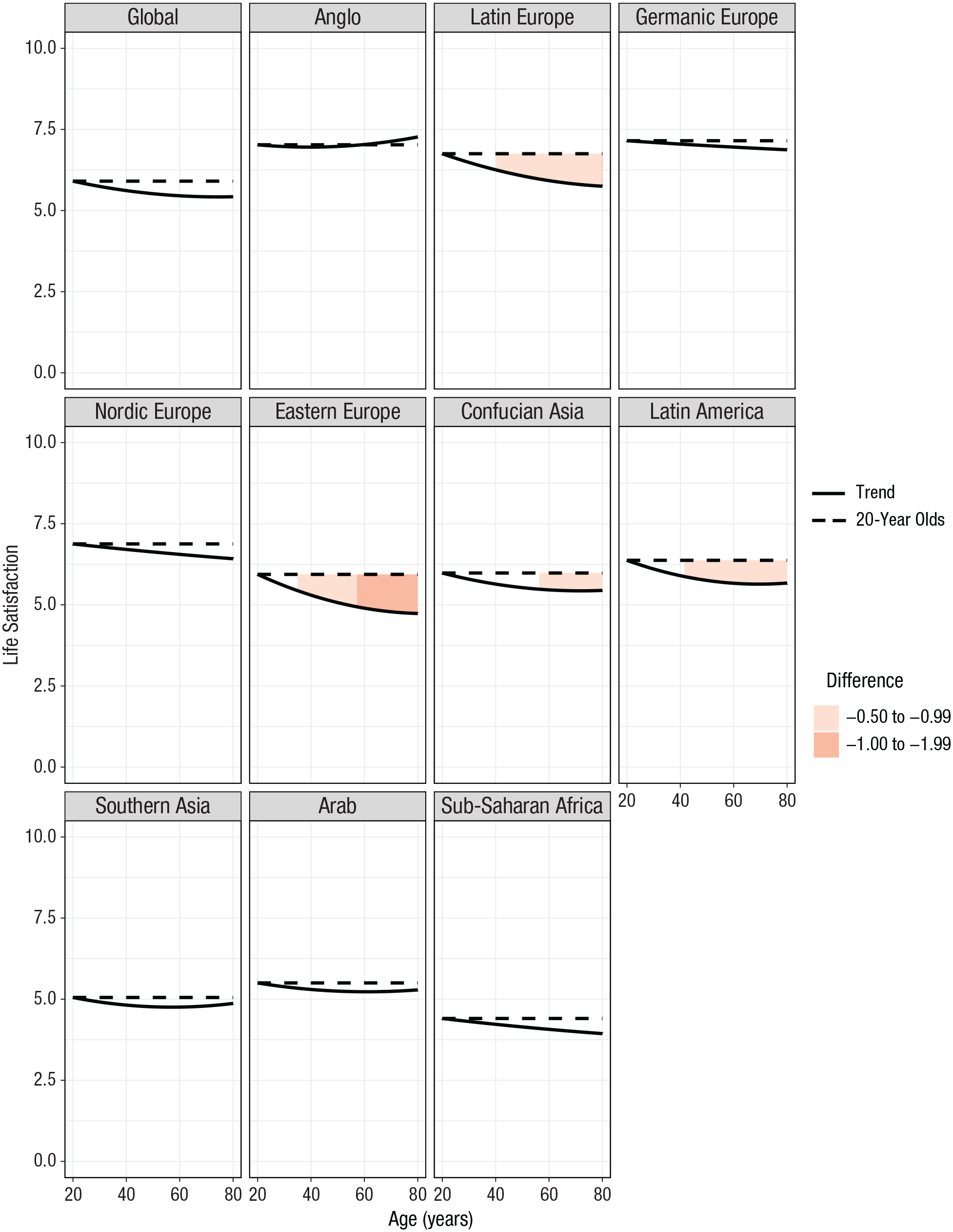
Predicted life satisfaction across the life span, globally and individually for each region. Each graph shows the overall trend and the trend for 20-year-olds only (baseline). Practically significant effect-size differences between the two trend lines are color coded.
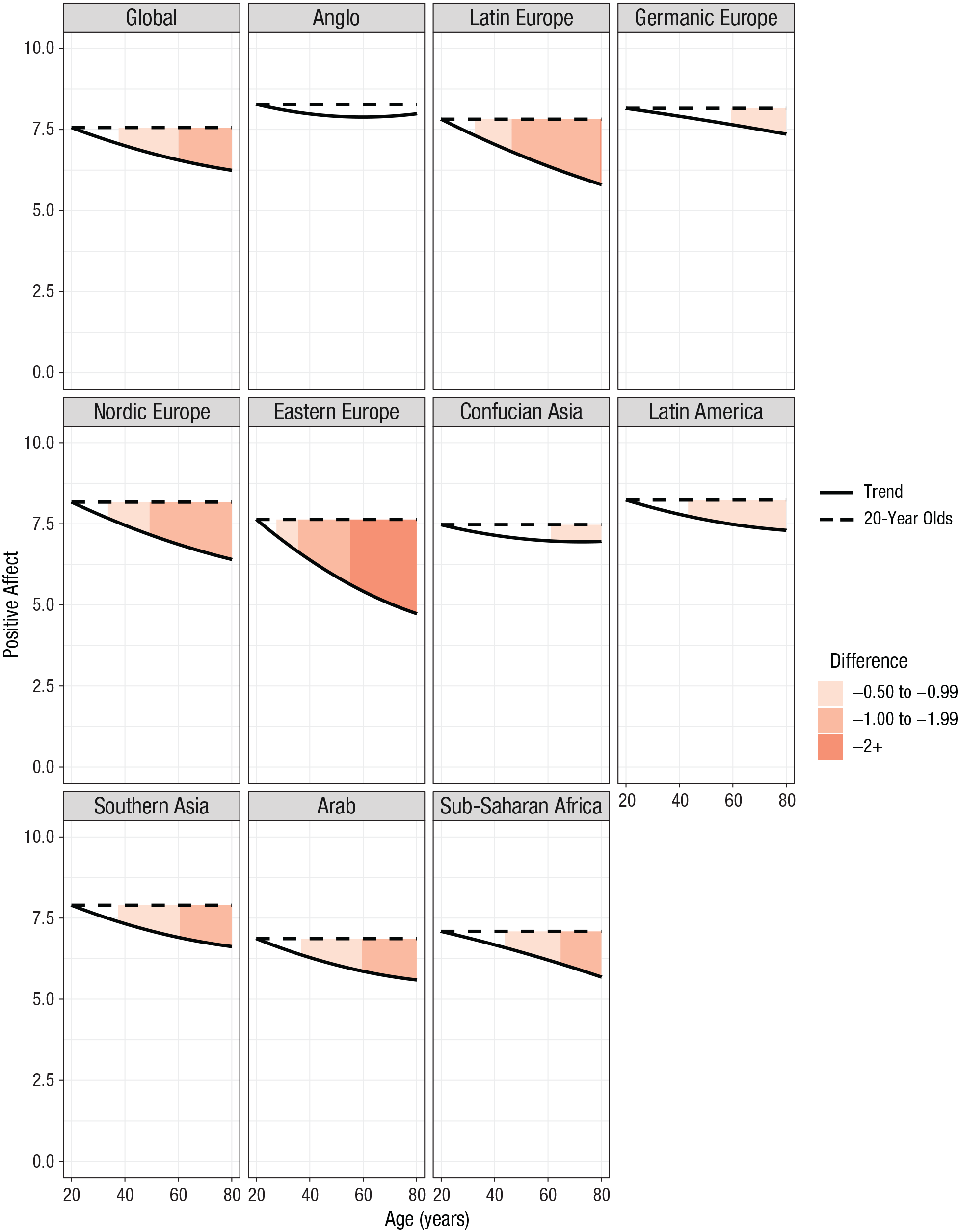
Predicted positive affect across the life span, globally and individually for each region. Each graph shows the overall trend and the trend for 20-year-olds only (baseline). Practically significant effect-size differences between the two trend lines are color coded.

Predicted negative affect across the life span, globally and individually for each region. Each graph shows the overall trend and the trend for 20-year-olds only (baseline). Practically significant effect-size differences between the two trend lines are color coded.
Supplemental issues: survey weighting, measurement validation, measurement invariance, and response styles
Finally, we examined a range of additional methodological issues, which are reported in the Supplemental Material. First, Gallup uses survey weights to correct for nonresponses (also called “sampling” or “probability” weights). A discussion of how these were used is provided. We also conducted a validity study to investigate the applicability of our Gallup measures. We found acceptable convergent validity. We then conducted measurement-invariance analyses and an analysis of the influence of responses styles across regions. We found that our multi-item measures were invariant and that response-style differences were not very significant across regions.
Results
Subjective-well-being trajectories across the life span
Table 1 gives correlations for the study variables. To explore changes of subjective well-being across the life span, we fitted a model with age and then examined how subjective well-being changed from 20 to 80 years of age. Model coefficients, model plots, and effect sizes (i.e., comparisons of 20-, 50-, and 80-year-olds) per region are available in Tables S2 through S4 and Figures S1 through S3 in the Supplemental Material.
Correlation Matrix of Study Variables

Note: All correlations were significant (ps < .001), except for those estimated to be zero. Correlations were computed with the nation-level mean removed from each observation.
Life satisfaction
Globally, the trend for life satisfaction was a negative curve (linear term: b = −0.01, p < .001; quadratic term: b = 0.0002, p < .001). However, all changes were very slight; they always stayed within 0.48 of the starting life-satisfaction score at age 20. This is displayed in Figure 1. When looking at the individual regions, one can see that most had changes that were similarly small (also in Fig. 1). One exception was Eastern Europe, where the decreases to life satisfaction reached 1.00 at age 60 and were 1.21 by age 80.
Positive affect
Globally, positive affect had a negative slope similar to the slope for life satisfaction over the life span (linear term: b = −0.02, p < .001; quadratic term: b = 0.0002, p = .008). However, unlike the effects for life satisfaction, the effects for positive affect were more practically relevant (see Fig. 2). The reduction in positive affect was 0.80 at age 50 and grew to 1.32 at age 80. Most of the regions were similar in form and effect-size magnitude. One exception was Eastern Europe, where the decreases were again much larger (1.76 and 2.90 at ages 50 and 80, respectively). Four regions also seemed to have smaller decreases over the life span (never reaching 1.00): Anglo, Germanic, Confucian Asia, and Latin America. To test this, we fitted a second model with dummy variables that coded these two groups of regions (and their product terms). The significant interaction meant that the slopes of these four regions were significantly less negative than the rest (Groups × Age: b = 0.02, p = .002; Groups × Age 2 : b = 0.00002, p = .89).
Negative affect
Globally, the curve across age for negative affect was statistically significant (linear term: b = −0.005, p = .004; quadratic term: b = 0.0001, p = .03), but the changes were all trivial (the maximum difference was a 0.28 increase at age 50 years). The results were slightly different for the regions individually (see Fig. 3). One group of regions was wealthier and had small decreases in negative affect: Anglo, Germanic, Nordic, and Confucian (the effect sizes ranged from 0.16 to 0.22 at age 50 years to 0.74 to 1.30 at age 80 years). The remaining six regions had small increases in negative affect: Latin Europe, Eastern Europe, Latin America, Southern Asia, Arab, and sub-Saharan Africa (effect sizes ranged from 0.42 to 0.74 at age 50 years and from 0.17 to 0.96 at age 80 years). Comparing these two groups of regions yielded a significant interaction in the expected direction (Groups × Age: b = −0.03, p < .001; Groups × Age 2 : b = 0.00007, p = .61). However, the changes within regions were almost all very small.
Predictors of subjective well-being
Next, we examined the role of predictors. For each of our four predictors, the global trends for all three outcomes are shown in Figure 4. (For coefficients, refer to the Supplemental Material.)
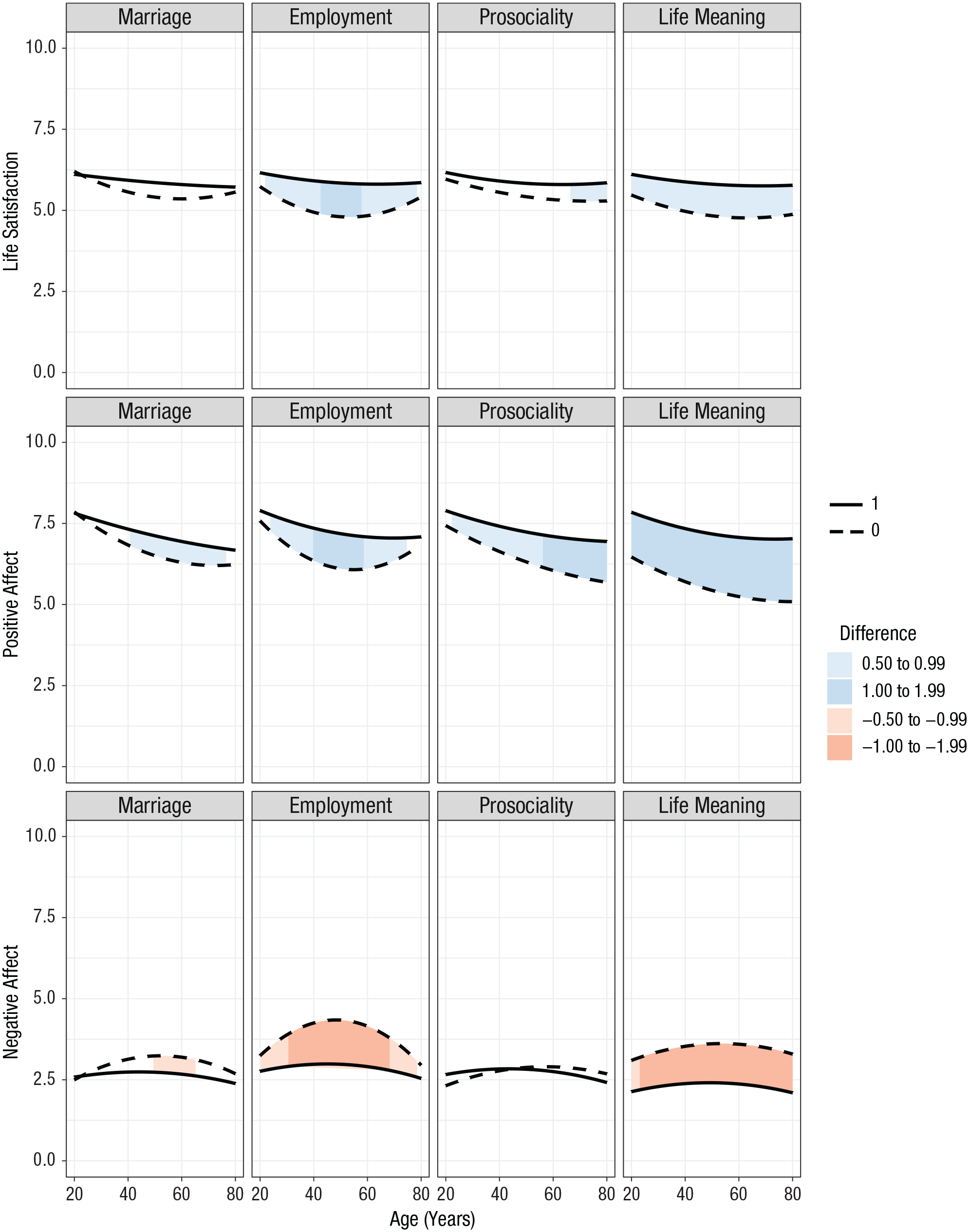
Global effect of each of the four predictors on the three subjective-well-being outcomes. Each graph shows the trends for the presence (1) and absence (0) of the respective outcome. Practically significant effect-size differences between the two trend lines are color coded.
Marriage
The first predictor we examined was marital status. Globally, for life satisfaction, there was a significant interaction between age and marriage; specifically, married people had slightly higher life satisfaction than unmarried people over the whole life span. However, the effect sizes across the life span were almost trivial; the largest difference was about 0.45 at age 50 years. This pattern was replicated in all of the individual regions; people who were married had higher life satisfaction, but these effects were all very small (never exceeding 0.76 in any region).
For positive affect, the same exact patterns were found. Globally and within each region, married individuals had higher positive affect across the whole life span, but these effects were also very small (the largest differences were roughly 0.61 at age 50).
Finally, we examined how marriage might be associated with reductions in negative affect. The results were the same as the other two measures of subjective well-being. Globally and regionally, unmarried people had slightly lower negative affect across the whole life span, but the effect sizes were all small (never greater than −0.67). For all three subjective-well-being outcomes, model coefficients for marriage and estimated effect sizes can be found in Tables S5 through S7, and plots of the Marriage × Age interactions are in Figures S4 through S6.
Employment
Next, we analyzed the effects of employment. There was a remarkable degree of consistency across the measures and regions. For all measures and regions, employed people had higher subjective well-being than unemployed people, with differences that usually peaked at around age 50 years and were lower at younger and older ages. The effect sizes were larger than for marriage and usually exceeded 1.00 by age 50 years. Globally, the effect sizes for life satisfaction at ages 20, 50, and 80 years were 0.43, 1.04, and 0.44, respectively. For the same ages, the effect sizes for positive affect were 0.32, 1.08, and 0.23, and for negative affect, they were −0.48, −1.36, and −0.41. There was some regional variation in these effect sizes, but all regions had qualitatively similar patterns. For all three subjective-well-being outcomes, model coefficients for employment and estimated effect sizes can be found in Tables S8 through S10, and plots of the Employment × Age interactions are in Figures S7 through S9.
Prosocial behavior
The next predictor we looked at was prosociality. Globally, people who engaged in prosocial behaviors had higher life satisfaction across the life span, but these effects were trivial in size, peaking at 0.56 by age 80. This functional form and effect-size magnitude was replicated for every region. For negative affect, there was no main effect of prosociality, and even though the interaction terms were both statistically significant, all effect sizes were trivial here as well (never exceeding −0.40). The only outcome with practical significance was positive affect. Globally, people who had been prosocial had higher positive affect over the entire life span; effect sizes grew continuously across age (0.52, 0.97, and 1.29 at ages 20, 50, and 80 years, respectively). The same functional form was present within each region with similar effect-size magnitudes. For all three subjective-well-being outcomes, model coefficients for prosociality and estimated effect sizes are in Tables S11 through S13, and plots of the Prosociality × Age interactions are in Figures S10 through S12.
Life meaning
Finally, the results of life meaning were very consistent. Across the entire life span and in every region of the world, individuals with life meaning had higher subjective well-being than those without life meaning. This was true for all three subjective-well-being measures. The effect sizes were practically significant and tended to grow across the life span. For ages 20, 50, and 80 years, the predicted mean differences were 0.64, 0.98, and 0.90 for global life satisfaction; 1.38, 1.74, and 1.94 for global positive affect; and −0.97, −1.20, −1.19 for global negative affect, respectively. The individual regions had similar effect sizes, with some variation. For all three subjective-well-being outcomes, model coefficients for life meaning and estimated effect sizes are in Tables S14 through S16, and plots of the Life Meaning × Age interactions are in Figures S13 through S15.
Discussion
Age differences in subjective well-being
Prior results are mixed on how subjective well-being differs across the life span (Ulloa et al., 2013), but many cross-sectional studies show a U-shaped curve with its low point around age 50 years (Blanchflower & Oswald, 2018). However, most of these studies examined only one subjective-well-being measure (life satisfaction), lacked worldwide samples, and did not take into account the practical significance of these differences. By contrast, our cross-sectional study examined three subjective-well-being measures in a representative sample from 166 countries and more than 1.7 million people. With these data, and accounting for practical significance, we found that much about the U shape has been overblown. Assuming that differences less than 1 scale point on a scale from 0 to 10 are small and approach being trivial, we found the only practical effects to be decreases in positive affect. Changes in life satisfaction and negative affect almost never exceeded 1 scale point in any region. In perhaps the most comprehensive study to date on the U-shaped curve, Blanchflower and Oswald (2018) examined seven large data sets. Two had life-satisfaction decreases from ages 20 to 50 years that were roughly 0.40 (United Kingdom) and 0.60 (32 European nations) on a scale from 0 to 10. 3 A scale from 0 to 5 was used in a third data set (41 nations), and doubling the decrease made it 0.60. In the remaining four data sets, either 3- or 4-point scales were used, so effect-size comparisons are more difficult, but the plots did not suggest any larger U shapes. In our study, the global decrease in life satisfaction was about 0.40 and ranged from 0.05 to 0.87 across regions. Therefore, although our conclusions differ on how prominent the U shape is, our data are consistent with past data, and the differing conclusions are a function of interpreting practical significance.
Positive affect, in contrast, showed practically significant decreases across the life span and reached 0.80 at age 50 years and 1.32 at 80 years globally. Regionally, we found that four regions (Anglo, Germanic, Confucian Asia, and Latin America) had smaller decreases, whereas the others had larger decreases, especially Eastern Europe. Interestingly, in 41 countries, Lucas and Gohm (2000) found that 3 countries with the largest positive-affect decreases were Eastern European (Poland, Czechoslovakia, and Romania) and that 4 with the smallest decreases were within the very same regions where we found decreases (West Germany, Austria, Ireland, Netherlands). For negative affect, we found that four wealthier regions had small decreases over the life span (Anglo, Germanic, Nordic, and Confucian), whereas other regions had small increases. Lucas and Gohm (2000) also found highly similar results.
Predictors of subjective well-being across the life span
With regard to marriage, we found highly consistent results: Across the whole life span, for all three measures of subjective well-being, and in every world region, married individuals had higher subjective well-being than unmarried individuals. These effects were consistently strongest at around age 50 and diminished toward both younger and older ages. However, all of these effects were very small, almost to the point of being trivial. The predicted mean difference between married and unmarried individuals never exceeded 0.76 for life satisfaction, 0.75 for positive affect, and −0.67 for negative affect, and most differences were smaller, as these were just the maxima. Helliwell, Norton, Huang, and Wang (2018) found that married individuals had higher life satisfaction in the United States (using the same measure) at every point over the life span, with similar effect sizes. Other studies found similar patterns, such as Grover and Helliwell’s (2019) United Kingdom study and Margolis and Myrskylä’s (2013) study, which found in data from over 90 countries that “partnership and children combined explain almost no variation over age in life satisfaction for most regions” (p. 123).
As with marriage, we found that individuals who were employed had higher subjective well-being across the entire life span for all three outcomes and all regions under study. These differences peaked at around age 50 years and were less at younger and older ages. Unlike with marriage, the observed effects were larger and had practical significance, usually exceeding 1 scale point at age 50. In a sample of 21 European countries, Lelkes (2008) found that employed individuals had higher life satisfaction than unemployed individuals at all ages, peaking also at around age 50 years, with a difference of roughly 1.50 on a scale from 0 to 10.
For prosociality, there were essentially no practically significant effects for both life satisfaction and negative affect for any region; the effect sizes were never greater than between roughly 0.62 and −0.40. By contrast, for positive affect, individuals who had been prosocial had higher mean levels over the entire life span, with effect sizes that reached 1.00 before age 60 years and grew continuously over the life span. This functional form was replicated for every region with a similar magnitude. Although the results were not replicated for life satisfaction, the finding with positive affect is consistent with socioemotional-selectivity theory, which posits that people reorganize their priorities as they age and place a greater focus on purposeful behaviors (Carstensen, Isaacowitz, & Charles, 1999).
Finally, the analyses of life meaning were very consistent in the same way for marriage and employment. Across the entire life span, in every region of the world, and for all three subjective-well-being measures, individuals with life meaning had higher subjective well-being than those without it. The effect sizes were larger, often exceeding 1 scale point. To our knowledge, no single study has examined how associations between life meaning and subjective well-being change across the life span in regions of the world. However, many studies have examined pieces and suggest a universality across age and cultures. For instance, life meaning has been found to be significantly related to subjective well-being across the whole life span (Reker, Peacock, & Wong, 1987) and to all three measures of subjective well-being (Steger, Oishi, & Kashdan, 2009), and it has significant associations in many world regions, including Latin America (Steger & Samman, 2012), Confucian Asia (Pan, Wong, Joubert, & Chan, 2008), sub-Saharan Africa (Temane, Khumalo, & Wissing, 2014), and Anglo (Steger et al., 2009) nations.
Limitations
The current study should be seen as a broad investigation into how subjective well-being differs across age and how it is associated with other variables. Thus, there are many more in-depth studies that can be developed, such as investigating what region-level variables predict age-trend differences or differences among countries within regions. In terms of study limitations, our data were entirely cross-sectional, which means that our age trajectories were not obtained from the same individuals tracked over time. We could not establish temporal precedence between our predictors and subjective well-being and must be more tentative about inferring causal relationships. There is also the possibility that cohort effects influenced observed age differences (e.g., 30- and 80-year-olds in our sample were raised in partly different circumstances). Many of our measures were also limited; for example, the prosociality and affect items did not assess their full domains (i.e., there are other prosocial behaviors and positive and negative emotions not included in our composites). Life meaning was assessed by one item only, which may lower reliability and attenuate the observed effects. Finally, the reader should note that our marriage and employment variables had several different subcategories (e.g., “unmarried” included individuals who were divorced, widowed, or have always been single, and “employment” included both full- and part-time work). The issue is that the prevalence of some subcategories may change with age (e.g., more widows and part-time workers at older ages), and this might underlie some of the observed changes in the effects. Readers should be mindful of this when interpreting the results, and future research should further examine underlying factors.
Conclusion
Overall, we found only very small differences in life satisfaction and negative affect across the life span, whereas decreases in positive affect were larger. Marriage had very small associations with subjective well-being, whereas employment had larger effects that peaked around age 50. Prosociality had practically significant associations only with positive affect, and life meaning had strong, consistent associations with all subjective-well-being measures across regions and ages. In all, our findings illustrate how different life priorities relate to our well-being as we age.
Supplemental Material
Morrison_Supplemental_Material – Supplemental material for Subjective Well-Being Around the World: Trends and Predictors Across the Life Span
Supplemental material, Morrison_Supplemental_Material for Subjective Well-Being Around the World: Trends and Predictors Across the Life Span by Andrew T. Jebb, Mike Morrison, Louis Tay and Ed Diener in Psychological Science
Footnotes
Transparency
Action Editor: Bill von Hippel
Editor: D. Stephen Lindsay
Author Contributions
A. T. Jebb analyzed the data. The first two authors wrote the manuscript, and all authors offered revisions. All of the authors approved the final manuscript for submission.
Notes
References
Supplementary Material
Please find the following supplemental material available below.
For Open Access articles published under a Creative Commons License, all supplemental material carries the same license as the article it is associated with.
For non-Open Access articles published, all supplemental material carries a non-exclusive license, and permission requests for re-use of supplemental material or any part of supplemental material shall be sent directly to the copyright owner as specified in the copyright notice associated with the article.