



Abstract
An impeller blower is one of the major aerodynamic noise sources in straw threshing machines. To reduce its aerodynamic noise, it is essential to understand the mechanism of gas-material-coupled unsteady flow causing aerodynamic noise. However, it is difficult to clarify the mechanism through measurement. Therefore, the following topics are studied in this article. First, a full-field transient numerical simulation of the gas and solid particulates’ unsteady flow inside the impeller blower was carried out using a dense discrete phase model and a large eddy simulation turbulence model. Second, based on the Ffowcs Williams–Hawkins equation, the aerodynamic noise of the impeller blower of the straw threshing machines was numerically calculated. Finally, the numerical results were verified by aerodynamic noise test. The results indicate that (1) sound pressure level at the inlet of the impeller blower is the highest, mainly at 100 Hz, which is the fundamental frequency of the rotating impeller, while the sound pressure level at the fourth harmonic frequency of 400 Hz is the main source of the outlet. The total sound pressure level at the inlet is greater than that at the outlet. It is concluded that the dipole source of the rotating impeller is the main noise source, which was generated by the interaction of blade with the air and material as the impeller rotated. Also, acoustic attenuation, acoustic resonance, and impact noise of material and machinery play important roles in aerodynamic noise distribution. (2) The test and simulation results show good agreement, so the numerical model of aerodynamic noise is reliable. This study will provide a reference for the structural and acoustic optimization design of impeller blowers and their integration into threshing machines.
Introduction
The straw threshing machine is a new type of forage processing equipment, which is mainly composed of a crusher and an impeller blower. The stalks are crushed by the crusher and thrown out by the blower. 1 A high noise level during the operation of straw threshing machines is a major problem. Previous research has shown that the noise from the impeller was the major source of noise from straw threshing machines.1,2 It affects not only the working performance and service life of the machine, but also the work environment, as well as the physical and mental health of the operators. 3
At present, research on noise from straw threshing machines mainly focused on experiments. Li et al. 1 and Wang 2 used experimental methods to analyze the noise of 9R-40 type straw threshing machines. They found that the blower is the main source of noise. Zhang et al. 4 measured and analyzed the noise of the blower under unloaded and loaded conditions and found that the main noise sources are aerodynamic and rotating noise. However, the cost of the experimental research method was relatively high and the research process was longer, so it was unclear how the throwing impeller disturbed the air and the material to cause the noise.
Research on noise created in similar rotating machines has been presented as follows. Kim et al. 5 studied the aerodynamic noise characteristics of Savonius wind turbine using the hybrid computational aero-acoustics technology. The proposed low-noise design used S-shaped blades which were found to reduce the noise levels of Savonius wind turbines by up to 2.7 dB. Mohamed 6 introduced an innovative design of the lift VAWTs (vertical axis wind turbines) to reduce the aero-acoustics noise emissions. Botha et al. 7 presented a method for predicting the aerodynamically generated broadband noise emitted by a VAWT. Four noise prediction models were implemented to determine the levels of inflow turbulence and self-noise produced by the turbine. Bazhenova 8 presented the results of theoretical and experimental studies of the occurrence and locations of aerodynamic noise sources in air blowers. These studies were based on basic research done by Lighthill and Curle and used an advance method for measuring pressure pulsations on rotating blades and stationary elements of a machine body. Chen et al. 9 employed the indirect boundary element method (IBEM) to study the noise of an industrial forward-curved centrifugal fan and to take the effect of volute reflection and scattering of the sound wave into consideration. A large eddy simulation (LES) was used to gain reliable pressure fluctuations on the surfaces of volute and rotating blades. Then, the Ffowcs Williams–Hawkins (FW-H) equation and Lowson equation were applied to calculate the dipole sources on the surfaces of the volute and the blades, respectively.
In this article, to identify the sources of aerodynamic noise production, theoretical analysis, numerical simulations, and experimental work are combined to study the aerodynamic noise of blowers in straw threshing machines, which provides a theoretical basis for the design of quieter straw threshing machines.
The rest of this article is organized as follows. Section “Analytical model” proposes the dense discrete phase model (DDPM) and the FW-H acoustic model for impeller blowers. Section “Numerical analysis of aerodynamic noise from the blower of the straw threshing machines” provides a numerical calculation and analysis method on the aerodynamic noise of impeller blowers. In section “Aerodynamic noise tests,” noise verification experiment is conducted. Finally, section “Conclusion” presents three conclusions.
Analytical model
DDPM model
Considering the volume fraction of the particles and the impact during their collisions, the DDPM describes the collisions statistically. In addition, the forces generated by collisions between particles are calculated according to the stress tensor of granular flow kinetic theory. The DDPM model is applied for problems with particulate higher volume concentrations, larger particle sizes, and inhomogeneous distribution of particles in the gas and when interphase drag forces play a dominant role.
In the DDPM model, the process for calculating the gas flow field uses the assumption of a continuous medium, and its law of motion is described by the Navier–Stokes (N-S) equations, in which the interphase mass and momentum transfer are considered. Because there is no mass transfer between the gas phase and the solid phase, the source term of the mass conservation equation is zero. The volume effects of the particulate phase in the DDPM model are described by the particles’ volume fraction and the air phase control equations 10



where αa is the volume fraction of the air phase of the gas–solid two-phase flow, as a percentage; ρa is the air density (kg/m3); t is the time (s);
The trajectory of the discrete solid particles is obtained by integrating the differential equations of their motion at discrete time steps in the Lagrangian coordinate system. The processes of integrating the kinetic equations introduce the interparticle collision forces and interphase forces. Considering that airflow pulsations will lead to strong turbulent diffusion, the varied pulsation velocity of the turbulence is introduced to show the influence of the turbulence on the particle trajectory. For gas flows with entrained solids, the effects of buoyancy and pressure gradients’ forces are assumed to be negligible. The kinetic equation of particle motion is then 10
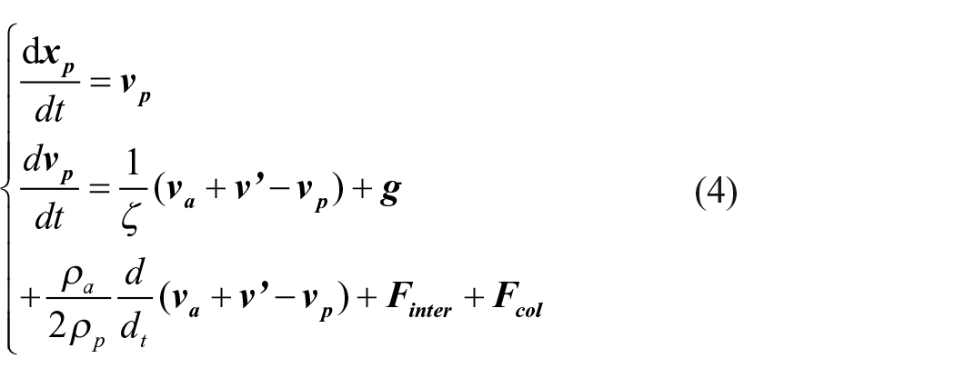
where
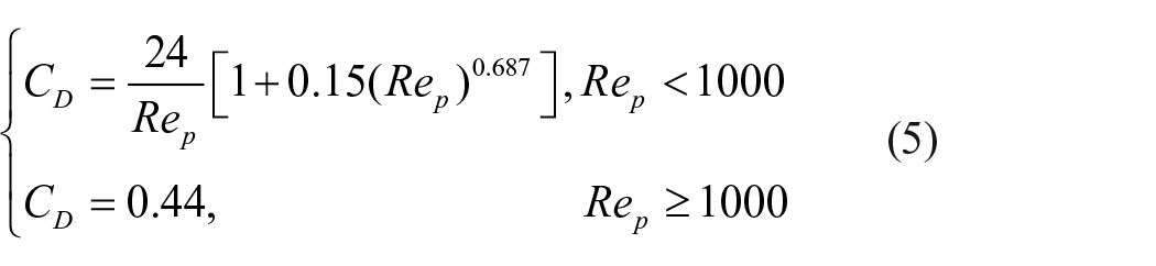
Each term in equation (4) is due to the forces exerted on the particles divided by the mass of the particles and can be regarded as contributions to the acceleration of the particles.
FW-H acoustic model
The internal flow field of the blower is complex, and its aerodynamic noise results from a number of factors. The far-field noise prediction for the blower is modeled using the FW-H equation. The FW-H equation models the noise generated by monopole, dipole, and quadrupole sources. The FW-H equation can be derived from the N-S equations and the continuity equation9,12 to yield
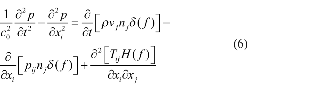
where c0 is the far-field sound velocity, p is the far-field sound pressure at time t, ρ is the far-field fluid density, nj is the normal vector of the structure surface, vj is the fluid velocity components in the xj direction, pijnj is the normal force per unit area acting on the fluid, δ(f) is the Dirac delta function, H(f) is the Heaviside step function, and Tij is the Lighthill stress tensor.
The first term on the right side of equation (6) represents the monopole sound source generated by the fluid volume displacement due to the impeller’s motion; the second term on the right side of the equation represents the dipole source generated by pressure fluctuations associated with unsteady airflow; and the third term on the right side of the equation represents the quadrupole source produced by viscous stresses.
The far-field noise of the blower is mainly attributed to a dipole sound source produced by the pressure fluctuations by the high-speed rotation of the impeller and the vibration of its shell. Because there is a relatively small fluid volume displacement within the impeller and the Mach number inside it is 0.2, the effects of the monopole sound source and the quadrupole sound source on total noise can be ignored.
The far-field sound pressure can be calculated using the generalized function theory and the free-space Green’s function to solve equation (6). The sound pressure at the far-field receiver location considering only the contributions from the dipole source is given by equation (7). A detailed derivation of equation (7) can be found in the work by Farassat 13

In equation (7),
The far-field sound pressure data are then obtained by post-processing the output of equation (7) with the fast Fourier transform (FFT) algorithm.
Numerical analysis of aerodynamic noise from the blower of straw threshing machines
The aerodynamic noise is closely related to the flow characteristics of the internal flow field in the blower. Computational fluid dynamics (CFD) software Fluent was used to numerically analyze the unsteady gas–solid two-phase flow field in the blower to obtain the pressure distribution of the internal flow field.
Numerical simulation of unsteady two-phase gas–solid flow in the blower
The motor power of the blower test bed is 5.5 kW. The impeller diameter is 500 mm, the blades’ width is 160 mm, and the blades are 5 mm thick. There are four blades, each with a blade pitch angle of 0°. The size of the inlet is 200 mm × 160 mm. The speed of the impeller is 1500 r/min. The blown material is corn stalks that were harvested in the suburbs of Hohhot in 2018. The material had an average density of 92.1 kg/m3. The material feed rate is 1.5 kg/s.
The three-dimensional (3D) modeling software CATIA was used to create the solid model of the blower, including the impeller and outer shell. The Boolean difference operation was used to create the moving model of the blower moving components. HyperMesh was used to divide the fluid mesh (Figure 1(a)) from the acoustic boundary element two-dimensional (2D) mesh (Figure 1(b)).

Schematic diagram of the impeller blower: (a) fluid grid and (b) acoustic boundary element mesh.
The internal flow field of the blower is part of a complex multiphase turbulent flow field. The DDPM in Fluent was selected for the calculation. The turbulent model uses the LES. 9 The implicit coupling algorithm is applied in the governing equations. The boundary conditions near the solid walls were analyzed using standard wall functions. The sliding mesh approach was used to simulate the relative movement between the impeller and the stationary components. The center of rotation was defined as the coordinate origin, the direction normal to rotation as the x-axis in the positive direction. The rotational speed was 1500 r/min. The inlet boundary conditions were set as a fixed velocity boundary condition: both the gas phase and the material phase had their velocity set to 15 m/s. The volume fraction of the solid phase was set to 0.2, and the solid material was assumed to be evenly distributed at the inlet. There was also air from the inlets of the bearing block gaps, with an air flow velocity of 5 m/s. The outlet boundary conditions used an outlet pressure boundary condition at standard atmospheric pressure.
To provide exact initial conditions for unsteady calculations and increase their convergence rate, steady state calculations are first run to convergence, and then the unsteady (turbulent) states are calculated. The time step for the solution is set to 1 × 10⁻⁴ s. The total time for each computation is 0.04 s (the period for the impeller to rotate a single revolution), so the number of time steps is 400 steps. The maximum number of iterations for each time step is set to 30. Considering the coupling between the discrete and continuous phases, the interference calculation for the discrete phase was performed after every 100 steps of the continuous phase. To track movement of the material, the maximum tracking step is set to 50,000 steps. The particles are set to enter the normal direction of the inlet at a speed of 15 m/s, with an average size of 0.0135 m and a flow rate of 0.5 kg/s.
Grid independency test
Compared with other different grids, it is found that the non-structural mesh used for this numerical calculation has better sensitivity and stability. 14 A grid independency test by calculating grid convergence index (GCI) 15 was conducted considering four non-structural grid sizes. The detailed steps for calculating GCI are as follows. 16
Define the grid convergence error σ as

In equation (8), i is 1, 2, 3, 4, and fi and fi + 1 are the numerical simulation results obtained when using the ith set and the (i + 1)th set of grids, respectively, and the simulation result is the flow field pressure.
Define the grid encryption ratio as

In equation (9), hi and hi + 1 are the average spacing of the ith and (i + 1)th sets of grids, respectively, and Ni is the total number of nodes per set of grids.
The definition of GCI is

In equation (10), Fs is the safety factor, the value range of which is between 1.25 and 3. When the grid used for evaluation is within two sets, the value is 3, and when more than three sets are used, the value is 1.25. p is the convergence precision, and its value can be obtained from equation (11) 14

In equation (11),
Equations (8)–(11) can be used to calculate the GCI. Four sets of grids are selected to evaluate the independence of the impeller blower’s grid. The maximum mesh size is changed to 20, 15, 10, and 5 mm by the Global Mesh setup in the meshing software ICEM to achieve the purpose of encrypting the mesh. The calculation results are shown in Table 1.
GCI calculation results.

GCI: grid convergence index.
It can be seen that the GCIs of the four grids with mesh sizes of 20, 15, 10, and 5 mm, respectively, are 9.75%, 1.97%, 0.43%, and 0.32%, with the last three sets of grids being less than 3%, which satisfies the GCI criterion. When the grid size is below 15 mm, the result of numerical calculation is independent of the number of grids. Increasing the number of grids will only bring a huge amount of calculation. The mesh size selected in this article is 15 mm, and the number of grids is 3.65 × 10⁶. Therefore, from the perspective of calculation time and efficiency, the grid size selected in this article is suitable.
Numerical calculations and analysis of aerodynamic noise of the blower
The main aerodynamic noise source of the blower is the dipole sound source. Considering the effect of the moving solid boundary of the impeller and the stationary solid boundary of the shell (including the outlet port and the inlet port) on the sound of the fluid, the static pressure wave is transformed into the dipole source representing the rotating impeller and the outer casing surface by the FW-H equation after the time domain fluctuating pressure on the surface by the impeller and the shell is obtained. IBEM in the acoustic software LMS Virtual.Lab Acoustic was used to calculate and analyze the radiation law for the aerodynamic noise from the blower, considering the impact of the shell over reflection and scattering of the sound field.
The data transmission between Fluent and LMS Virtual.Lab Acoustic was carried out by the CFD general notation system (CGNS). The parameters of the unsteady flow field were used to solve for the sound field, with the number of time steps being set to 1200 (about three cycles).
The aerodynamic noise field grid is defined as an ISO standard hexahedron field with a refinement level of 15. To compare with the measured values, two mutually perpendicular plane field points are added at the inlet and the outlet. The outer intersection of the two plane field points at the entrance corresponds to the test point R1 (1.083, 0, and −0.155), and the outer intersection of the two plane field points at the exit corresponds to the test point R2 (0, 1.826, and 0.928).
Analysis of the sound pressure level cloud chart for the hexahedron field
The sound pressure of the blade passing frequency (BPF) and its harmonic frequencies at the far-field receiver’s location in the hexahedron field were obtained, and the first six order sound pressure levels’ (SPLs) cloud images are shown in Figure 2. The sound pressures are the A-weighted SPL, and its unit is dB(A).
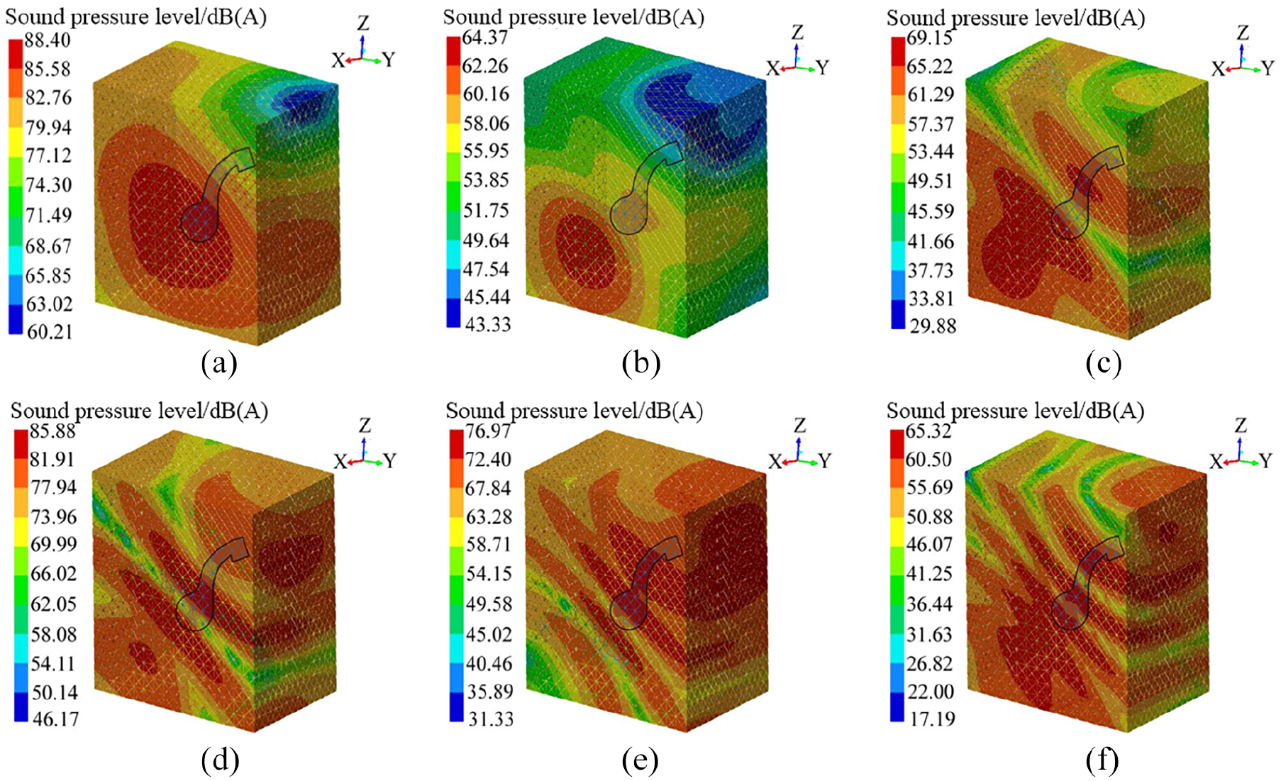
First six order SPL cloud chart of hexahedron field.
It can be seen from Figure 2 that the aerodynamic noise is higher and mainly concentrated at the inlet, at a base frequency of 100 Hz and a second harmonic frequency of 200 Hz. The higher SPL of the third harmonic frequency of 300 Hz was mainly concentrated at the inlet and at the side of the outlet pipe. The higher SPLs at 400, 500, and 600 Hz were mainly concentrated at the inlet, the side of the outlet pipe, and the outlet. Comparing the SPL cloud maps of these six frequencies, the area of the region with the highest SPL at 100 Hz is the inlet, and the maximum SPL is 88.40 dB(A), which is the highest SPL of all highest sound. The area of the region with the highest SPL at the outlet has its peaks at 400 and 500 Hz, and its maximum SPL at 400 Hz is 85.88 dB(A), which is the second highest SPL at those frequencies. It can be seen that the largest contribution to the total noise from the blower is at 100 and 400 Hz. The SPL at the inlet is mainly affected by the SPL at 100 Hz, and the SPL at the outlet is mainly affected by the SPL at 400 Hz. The maximum value of the SPL at other frequencies is nearly 10 dB(A) less than the secondary peaks at 100 and 400 Hz.
This is mainly because the dipole source of the rotating impeller is the main noise source which was generated by the interaction of the blade with the air and material in a periodical pattern as the impeller rotated. The excitation frequency of the impeller for two-phase flow field was computed as 17

In equation (12), n is the rotational speed of the impeller, n = 1500 r/min. Z is the number of blades of the impeller, Z = 4. Index i is the harmonic number, i = 1, 2, 3, . . . The index i = 1 refers to the fundamental frequency of 100 Hz. The second harmonic was 200 Hz (i = 2), the third harmonic was 300 Hz (i = 3), and so on. The exciting energy at the fundamental frequency of the impeller was the largest, 17 so the highest SPL appeared at 100 Hz. The noise is directly radiated from the inlet and the attenuation of this noise is weak, whereas the outlet is far away from the sound source (the rotating impeller), so the noise passed through the outer housing of the rotating impeller and outlet pipe and then radiated outward, resulting in attenuation of noise along the noise transmission path. In addition, because the straw is not broken when fed into the machine, it will cause impact noise at the inlet and make the SPL at the inlet larger than that at the outlet. As can be seen in Table 2 of the resonant frequencies and in Figure 5 of the vibration diagram of the acoustic modal, the propagation of sound waves of different frequencies in the impeller blower is not only affected by the frequency of the sound waves (the higher the frequency, the greater the attenuation of sound pressure) but are also affected by the acoustic modal characteristics of the blower device. The deviation between the fourth harmonic frequency of 400 Hz and the fifth-order acoustic modal-resonance frequency of 372.023 Hz is only 7.0%, and the deviation is only 7.6% from the sixth-order acoustic modal-resonance frequency of 430.414 Hz, so the sound resonates through the outer casing and the outlet pipe, and the SPL of the blower increases. In short, the SPL at the fundamental 100 Hz is the highest at the inlet due to its greater energy and lesser attenuation and the impact noise of material and machinery. The SPLs for 400 Hz at the outlet increase due to the acoustic resonance at that frequency.
Resonance frequency of acoustic modal.
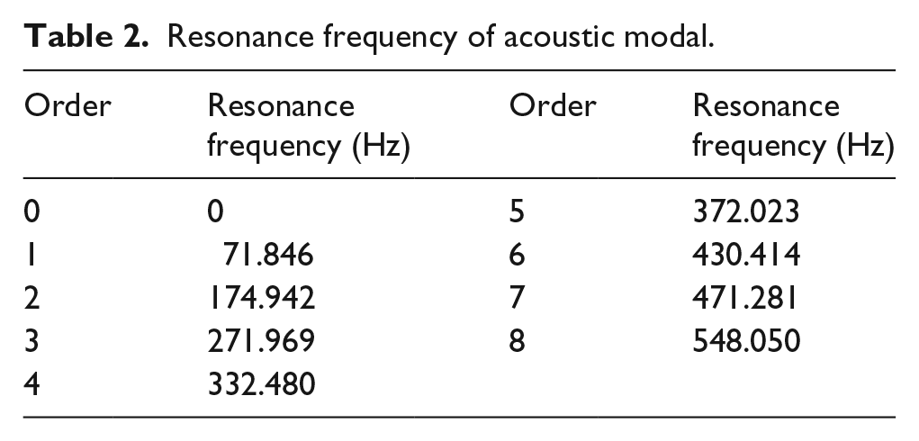
The variations of SPLs are 28.19, 21.04, 39.29, 39.71, 45.64, and 48.13 dB(A), respectively, at 100, 200, 300, 400, 500, and 600 Hz. It can be seen that as the frequency increases, the variation of the SPL increases, and the radiation of the noise gradually becomes disordered and varied. This is mainly due to the fact that as the frequency increases, the noise radiation at the outlet increases, and the superposition of the noise radiation from the outlet and the inlet gradually becomes apparent. The characteristics of acoustic modes of the device are more complicated with the frequency increases as shown in Table 2 and Figure 5, which cause the characteristics of noise radiation with higher frequencies to be more complicated.
Analysis of SPL nephogram for intersecting plane fields
The SPL cloud chart of the intersecting plane field spots at the inlet and the outlet of the blower is shown in Figure 3.

First six order SPL cloud chart of the intersecting plane field spots.
It can be seen from Figure 3 that at the inlet, the variations of the first six harmonics of the SPL cloud map are basically similar. Besides rippling radiation, there are also many abrupt changes (green was changed to blue) in the distribution diagrams for the SPLs at the outlet. The mutation regions are all lower sound pressure regions. This is due to the attenuation caused by the interference during the propagation of sound waves passing through the housing and outlet pipe. For the frequency of 100, 200, and 300 Hz, the SPLs at point R1 of the inlet are higher than the SPLs at point R2 of the outlet; for the frequencies of 400, 500, and 600 Hz, the SPLs at point R1 are lower than the SPLs at point R2. At frequencies of 500 and 600 Hz, the differences between the SPLs at the inlet and the outlet are small. The SPL at the inlet is mainly affected by the sound’s radiation attenuation and the impact noise of material and machinery. The energy of lower frequency noise was larger, and the noise attenuation was weaker at the inlet than at the outlet, so the SPLs at 100, 200, and 300 Hz at point R1 are higher than those at point R2. Besides that, the SPL at the outlet is affected by multiple reflections and superpositions of the shell and outlet pipe. The deviations are less than 9% between higher excitation frequencies of 400, 500, and 600 Hz and acoustic modal-resonance frequencies from the fifth order to the eighth order (the deviation is 7.0% between 400 Hz and the fifth-order acoustic modal-resonance frequency of 372.023 Hz; the deviation is 7.6% between 400 Hz and the sixth-order acoustic modal-resonance frequency of 430.414 Hz; the deviation is 6.0% between 500 Hz and the seventh-order acoustic modal-resonance frequency of 471.281 Hz; the deviation is 8.7% between 600 Hz and the eighth-order acoustic modal-resonance frequency of 548.050 Hz). So the sound resonates through the outlet pipe, and the SPL at 400, 500, and 600 Hz at the outlet increases. Furthermore, it could be seen that resonance occurs twice at 400 Hz (400 and 372.023 Hz, 400 and 430.414 Hz) and once at 500 and 600 Hz, respectively, so the SPL at the outlet is mainly affected by the SPL at 400 Hz, as can be seen from Table 2.
SPL spectral analysis
The acoustic pressure level spectrogram of the two measuring points R1 at the inlet and R2 at the outlet can also be represented by a 2D curve, as shown in Figure 4(a) and (b) (simulation).
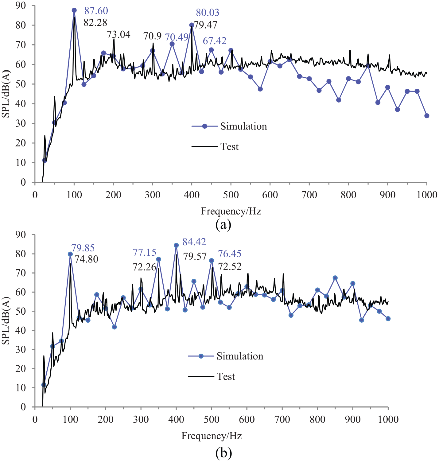
Comparisons between the measured auto-spectrum analysis and the simulation SPL spectrogram of at the measurement points.
It is generally believed that two SPLs with a difference of more than 10 dB(A) are added, and the influence of the smaller SPL on the result is negligible. Therefore, the effective peaks of the point R1 are the SPLs at 100, 400, 350, and 450 Hz, and the effective peaks of the point R2 are the SPLs at 400, 100, 350, and 500 Hz. The SPLs at 100 Hz at the inlet and 400 Hz at the outlet contribute the most to the total sound pressure level (TSPL). The SPL spectrum of the exit point is similar to the SPL spectrum of the inlet point, because the noise at both points is radiated by the same noise within the impeller, so the basic characteristics are similar.
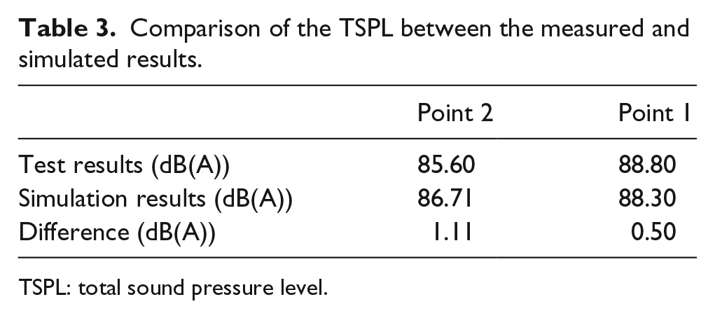
When calculating the TSPL, only the SPL of each effective peak is considered. According to the SPL superposition equation (9), the TSPL at the outlet measuring point is 86.71 dB(A), and the TSPL at the inlet measuring point is 88.30 dB(A). The TSPL at the inlet is greater than the TSPL at the outlet due to acoustic attenuation, acoustic resonance, and impact noise of material and machinery

In equation (13),
Acoustic modal calculation and analysis
The propagation of sound waves within the blower is mainly affected by the blower’s structural parameters and the position of the sound source. Acoustic modal analysis is an effective way to model the sound propagation in the device. To better understand the radiation characteristics and aerodynamic noise of the device, the acoustic modal of the blower was simulated using the finite element method, in the LMS Virtual.Lab Acoustic software package. The sound pressure values at the resonance frequencies of the acoustic modal in Table 2 are shown in Figure 5.
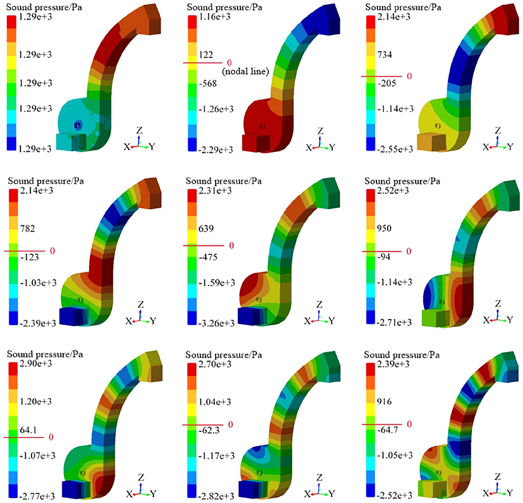
Vibration diagrams corresponding to different acoustic modes.
It can be seen from Figure 5 that although the zero-order modal results show a cloud image change, the sound pressure values of each color blocks are consistent, so it is a zero-order modal. The fundamental frequency sound pressure mode is mainly distributed in the Z-axis direction, and there is only one nodal line (i.e. the color band with zero sound pressure). The second harmonic sound pressure mode is mainly distributed along the Z-direction, and there are two nodal lines. The third harmonic sound pressure modal is also mainly distributed along the Z-direction, and there are three nodal lines. The fourth harmonic sound pressure mode is mainly distributed along the Z-axis and X-axis directions, as shown by the three Z-direction nodal lines and single X-direction nodal line. The fifth harmonic sound pressure mode is distributed along all three coordinate axes, as illustrated by the three Z-directional, one X-directional, and one Y-directional nodal lines. The sound pressure distributions of the sixth to eighth nodes were more complicated and were combinations of Z-direction, X-direction, Y-direction, and circumferential distribution. This is mainly because the outlet pipe is a typical panel structure and the acoustic-vibration resonance would occur within pipe.
Aerodynamic noise tests
Testing instruments and methods
The experimental equipment included a TES-1352A programmable noise meter (with testing scope of 30–130 dB(A)), an INV3060S signal acquisition analyzer, DASP V10 analysis software produced by China Orient Institute of Noise and Vibration, and a computer. The testing conditions are the same as the numerically modeled conditions. An open area was used for the test site, and the test bench was fixed on the ground with expansion bolts.
The measuring point arrangement for aerodynamic noise measurements refers to the Chinese National Standard GB6971-2007 for noise measurements in straw threshing machines. The pneumatic noise from the blower mainly consists of noise at the inlet and the outlet. When measuring noise at the inlet, the measurement at point 1 (same as R1) is on the axis of the inlet, at a distance from the center of the inlet of 1 m. When measuring the noise at the outlet, point 2 (the same as R2) is in the direction of 45° from the axis of the outlet, at a distance from the center of the outlet of 1 m, as shown in Figure 6(a).
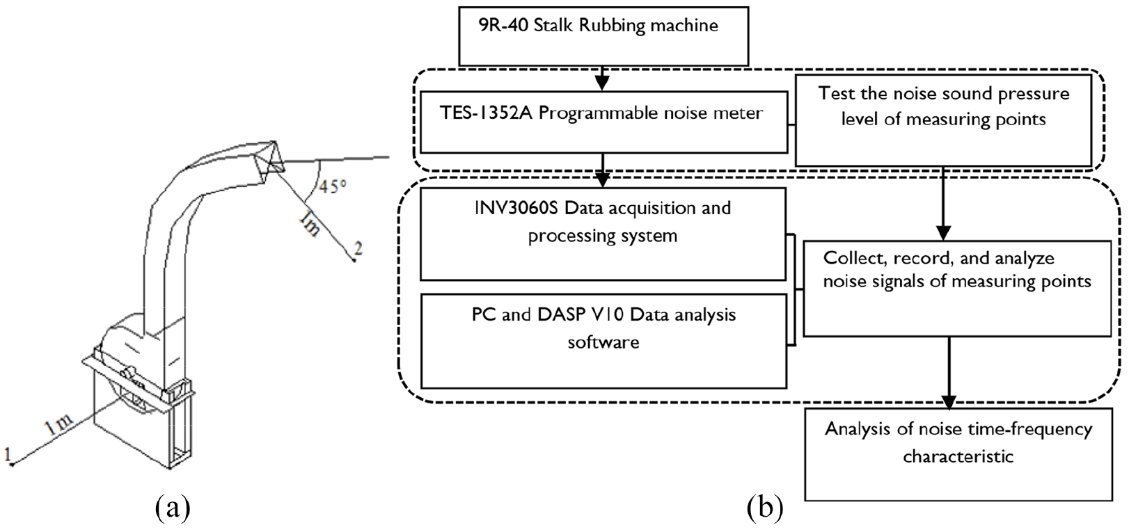
Pneumatic noise measurement point arrangement and test procedure.
The SPLs measured at points 1 and 2 are shown in Figure 6(a) under load conditions, as measured by the microphone of the TES-1352A programmable noise meter. The signal acquisition analyzer INV3060S collected and recorded the noise signal, which is then analyzed using DASP V10 software on the PC. For testing, the sensitivity of microphone was set to be 30 mV/Pa in DASP V10 and the sampling time was set to 30 s. The analysis parameters are A-weighted, and the Hanning Window filtering function was used. The sampling frequency was 51.2 kHz, and the input type was integrated circuits piezoelectric (ICP). The flow chart for the noise tests and analysis are shown in Figure 6(b).
The background noise of the motor and test site was first tested with results of 65 and 57 dB(A). The difference between the background noise and the average noise of the device of 84.7 dB(A) was greater than 10 dB(A), so the influence of background noise on the test data and measurement process was not considered.
Analysis of test results
The noise measurement results under load for the two test points in Figure 6(a) are shown in Table 3. As can be seen from Table 3, the noise at the inlet was larger than at the outlet. The auto-spectrum analysis of the noise signals for the two measuring points was performed separately. The spectral form used the amplitude spectrum peak, and the Hanning window function was used. The ordinate was displayed as the A-weighted SPL, as shown in Figure 4 (test).
Comparison of the TSPL between the measured and simulated results.
TSPL: total sound pressure level.
It can be seen from the auto-spectrum analysis of the two measuring points in Figure 4 (test) that the spectrum structures for measuring point 1 and measuring point 2 are very similar, and the main noise frequencies were composed of both discrete spectrum and continuous spectrum. Discrete noise is also called the rotation noise which was generated by the blade interacting with the air and material in a periodical pattern as the impeller rotated.
It can be seen from Figure 4 (test) that the main frequency of measuring point 1 and that of measuring point 2 are both fundamental frequency 100 Hz, and there are obvious peaks at harmonic frequencies. It can be seen that the main noise is the rotating noise. It can be seen from Figure 4(a) that the SPLs of measuring point 1 are larger at 100, 200, 300 and 400 Hz, and their differences are obvious. The SPLs of measuring point 2 are larger and around 70 dB(A) between 100 and 700 Hz as shown in Figure 4(b).
In summary, the SPL at the inlet of 100 Hz is higher than that at other areas, and the SPLs at 100–700 Hz at the outlet are high and very close to one another.
It is mainly due to the noise being radiated from the sound source (mainly the rotating impeller) directly to the inlet, and the attenuation of the noise is relatively small, so the acoustic pressure level at the 100-Hz inlet is higher. The radiated noise through the outlet is intense and similar because of the combined effects of acoustic attenuation and acoustic resonance, as shown in Figure 5.
Comparative analysis of the numerical and measured results
The comparison of the TSPL between the numerical and measured results for aerodynamic noise at the inlet and the outlet is shown in Table 3.
It can be seen from Table 3 that when comparing the test results with the simulation results, the difference between the simulated and measured TSPLs at the outlet is 1.11 dB(A), and the difference at the inlet is 0.50 dB(A). The errors between the test result and the simulation result were both small.
Comparing the SPL spectrogram and the auto-spectrum analysis in Figure 4, it can be seen that although the frequency of the data points in the simulated spectrum is only 25 Hz and its multiples and the spectrum of the simulation results are relatively simple, the variation law and the values of the main data points are basically consistent with the auto-spectrum analysis results of the measured value at the outlet. The simulated effective peaks and measured ones at the outlet are both the SPLs at 400, 100, 350, and 500 Hz. The maximum difference between the simulated effective peaks and experimental ones is 5.05 dB(A). The simulated effective peaks at the inlet are the SPLs at 100, 400, 350, and 450 Hz, while the measured effective peaks at the inlet are the SPLs at 100, 400, 200, and 300 Hz, the differences in the main effective peaks between the simulated and measured ones at 100 and 400 Hz are 5.32 and 0.56 dB(A), respectively. There is a big difference between the simulated SPLs and measured SPLs at high frequencies.
There were several causes for the deviation between the simulated and experimental values: (1) the straw is not broken when fed into the machine, and it will cause impact noise at the inlet while the simulation model has not taken this into account; (2) the dipole source was only considered in the simulation model, and the monopole and the quadrupole sound sources were not considered; and (3) measurement errors are inevitable in the test.
In summary, the simulated results for the aerodynamic noise in the blower are basically consistent with the experimental results. This serves to verify the credibility of the calculated results.
Conclusion
In this article, the aerodynamic noise of the blower of straw threshing machines was numerically calculated using the hybrid acoustic calculation method, based on the acoustic analogy theory FW-H equation. The SPL cloud map, the SPL spectrum map of the measuring point, and an acoustic modal analysis were adopted to analyze the aerodynamic noise radiation of the blower, and the numerically predicted results were verified by the aerodynamic noise tests. The results of research indicated the following:
The total noise of the impeller blower is mainly affected by the SPL of the rotating impeller at its fundamental frequency of 100 Hz and its fourth-order frequency of 400 Hz. The SPL at the inlet is mainly affected by 100 Hz, and the SPL at the outlet is mainly affected by 400 Hz. The TSPL at the inlet is greater than the TSPL at the outlet. As the frequency increases, the variation of the SPLs increases gradually, and the characteristics of the noise’s radiation gradually become disordered.
The patterns of the variation of the SPL cloud chart at the inlet of the blower are basically similar, but the SPL cloud diagram at the outlet is mainly composed of the rippling radiation with more areas with low SPLs. At frequencies of 100, 200, and 300 Hz, the SPLs at the inlet are greater than the SPLs at the outlet. The SPLs at the inlet at frequencies of 400, 500, and 600 Hz are less than the SPLs at the outlet.
The calculated TSPL at the outlet is 86.71 dB(A), and the difference from the measured TSPL of 85.60 dB(A) is 1.11 dB(A). The calculated TSPL at the inlet is 88.30 dB(A), and the difference from the measured TSPL of 88.80 dB(A) is 0.50 dB(A). The discrepancies between the test results and the simulation results are small, and the variation of the spectrum of the simulation results and its main peaks are basically consistent with the auto-spectrum analysis of the test results. It can be seen that the simulation results for the aerodynamic noise in the impeller are credible, and the numerical model forecasting the aerodynamic noise from the blower is accurate.
Footnotes
Declaration of conflicting interests
The author(s) declared no potential conflicts of interest with respect to the research, authorship, and/or publication of this article.
Funding
The author(s) disclosed receipt of the following financial support for the research, authorship, and/or publication of this article: This research was supported by the Inner Mongolia Natural Science Foundation (No. 2018MS05059) and Inner Mongolia Autonomous Region Science and Technology Plan Project (2019).
