The greenhouse gas impact of bioenergy in developing economies: Evidence from Taiwan

Abstract

Greenhouse gas emission induced global climate shift is an immediate threat to the world because of increased likelihood of the occurrence of extreme events. Expanding bioenergy production on currently set-aside land is an attractive option being considered by Taiwanese policymakers to reduce potential damages. This study investigates the impact of pyrolysis-based bioelectricity and ethanol on the greenhouse gas emission using a two-stage dynamic semi-parametric model. The results show that the bioelectricity generation has a significantly positive impact on the emission reduction. It encourages Taiwan to place more public resource on bioelectricity generation. This study is extended to forecast the emission reduction for 2015 to 2017. The quarterly emission reduction forecasts vary between 214,806 and 239,497 tons, which is less than 3% out of total emissions. It implies that the Taiwanese government could move the policy supports from biofuel production to bioelectricity production to reduce greenhouse gas emissions.

Keywords

Bioelectricity ethanol greenhouse gas emission policy analysis pyrolysis

Introduction

Bioenergy is considered an effective way to mitigate greenhouse gas (GHG) emissions. For example, Schneider and McCarl¹ compare the effects of GHG emissions of conventional bioenergy technologies, and Haberla et al.² correct the fundamental error in GHG accounting related to bioenergy. Many studies related to bioenergy and GHG emissions have also been conducted.^3–6 Bioenergy and emissions reductions have been investigated in terms of climate change mitigation and change in social welfare and farmers’ revenue, but the economic relationship between bioenergy production and GHG emissions has rarely been surveyed.

In 2002, Taiwan became a member of the World Trade Organization, and consequently, approximately one-third of agricultural cropland has been released due to its lower competitive power. To better utilize the released land and enhance farmers’ income, the Taiwanese government adopted the Renewable Energy Development Plan in 2002 aiming at not only generating energy domestically but also supporting farmers. Murray et al.⁷ employ energy-economic models and diagnose the effect of the federal tax code on GHG emissions. They find that bioenergy tax (or subsidy) policies have little impact on reducing GHG emissions in the US, but their findings do not consider the relationship between energy prices, bioenergy production, and GHG emissions. Ozturk⁸ uses a dynamic heterogeneous panel model to investigate the dynamic linkages between biofuels production and GHG emissions in 17 countries from 2000 to 2012. These results confirm that biofuel production increases along with total GHG emissions. However, GHG emissions considered in this study include emissions from “ALL” sectors such that the results cannot reveal any relationship between bioenergy production and emissions effects of specific types of biofuel. Moreover, this study does not provide any indication of how bioenergy production influences GHG emissions. These findings provide some information to the Taiwanese government in support of investigating the feasibility of its own bioenergy industry. However, the main purpose of current bioenergy development is to reduce expenditures on costly imported foreign energy.^9,10

This study aims to investigate and explore how the reduction of GHG emissions can be influenced by bioenergy products, such as ethanol production and electricity production, and by relevant economic factors, such as gasoline prices, coal prices, and GHG prices. Because ethanol and electricity production may be endogenous, a two-stage dynamic semi-parametric regression is proposed in this study.

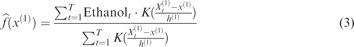
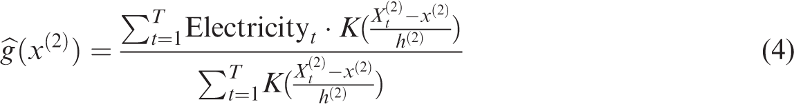
In the first stage, each explanatory variable that is an endogenous covariate in the equation is regressed on all of the exogenous variables in the model, including the exogenous covariates, which are coal, gasoline and GHG prices, and the instrumental variables, which are lagged ethanol and electricity generation.^a In this stage, we employ nonparametric kernel regression instead of parametric regression to avoid a possible model misspecification. The predicted values for these regressions are obtained. In the second stage, the dynamic linear regression of interest is estimated as usual, except that each endogenous covariate is replaced with the predicted values from the first stage.

The results show that GHG prices have a significant positive impact on the reduction of GHG emissions at a 1% significance level. The reduction of GHG emissions increases by 0.41% when GHG prices go up by 1%. Meanwhile, our study also finds that electricity generation has a positive impact on the reduction of GHG emissions. As electricity generation increases by 1%, GHG emissions reduction increases by approximately 0.48%. The estimated parameters of coal and gasoline prices are insignificant, implying that coal and gasoline prices may not have a direct influence on reducing GHG emissions.

To demonstrate the robustness of our model, this study develops an alternative two-stage dynamic semi-parametric model with the same covariates, except that coal and gasoline prices are treated as instrumental variables. Our alternative model reports similar estimations, indicating the robustness of our model.

Moreover, because climate change mitigation could last for many years, it is therefore necessary for the government to examine both present and future emissions when making sustainable environmental policies. This encourages us to extend the reduction forecast period in our study to include the period from the second quarter of, 2015 to the fourth quarter of 2017. To verify forecasting accuracy, this study evaluates out-of-sample performance in terms of the mean forecasting error (MFE) and mean absolute percentage error (MAPE). The results of MFEs demonstrate that the proposed model tends to under-forecast reductions in GHG emissions, which is not a critical problem as under-forecasted the reduction of GHG emissions can persuade the government to make more efforts to achieve the intended target. Meanwhile, the evaluated MAPE is less than 1%, revealing a convincing forecasting performance of the proposed model.

The forecasts of the quarterly reduction of GHG emissions vary between 214,806 and 239,497 tons based on the proposed model. To enable a comparison, a conventional mathematical optimization model is employed. The forecasts of reduction of GHG emissions vary between 194,359 and 308,766 tons based on the mathematical model. The volatility of forecasted reduction of GHG emissions in the proposed model is lower than that in the mathematical optimization model. The average percentage error of forecasted reduction of GHG emissions between the proposed model and the mathematical model is 4.21%, implying that the proposed model is capable of replacing the mathematical optimization approach in terms of forecasting the reduction of GHG emissions.

The forecasted annual emissions reductions are less than 3% of total emissions,^b and include only less than half of released land participating in current bioenergy programs. These results indicate that the Taiwanese government could increase financial subsidies or rewards to shift land use to bioenergy, especially bioelectricity. Potential incentives to increase participation of the whole supply/demand chain in bioelectricity generation include a more generous subsidy for energy crop plantation to compensate for the higher marginal production cost of farmers, higher tax credits or benefits to bioelectricity producers, and establishment of an emissions trading system that allows bioenergy producers to realize the gains from GHG emissions offsets. However, measurement and monitoring of net GHG emissions may be difficult and will require government intervention.

Our work contributes to the extensive literature on GHG emissions in the following ways. To the best of our knowledge, our study is the first to discuss how economic and bioenergy factors influence the reduction of GHG emissions in terms of an econometric framework. The estimated results demonstrate the importance of electricity generation when reducing GHG emissions, justifying the merits of the proposed model.

Secondly, our study forecasts emission reductions using the proposed framework. In contrast to the complex mathematical programming model, our econometric model provides a parsimonious approach with convincing accuracy to forecast the reduction of GHG emissions. In other words, government analysts should be able to use our model to evaluate the emissions reduction given a certain level of bioenergy production and market prices.

This paper proceeds as follows. “Literature review” section contains the literature review. “Data and variables description” section describes the data and variables selected based on a mathematical programing model. “Methodology” section introduces the econometric model. “Empirical study” section presents the empirical results. “Forecasting of the reduction of GHG emissions” section presents a simulation of emissions reduction forecasts. “Concluding remarks” section concludes the study.

Literature review

The Intergovernmental Panel on Climate Change (IPCC) has concluded that human activity is at least partly responsible for the increase in global mean temperatures over the last century.¹¹ Because climate change impacts forest productivity and species distributions¹² as well as the world food supply,¹³ it is associated with substantial risks for society and nature.¹⁴ As Metz et al.¹⁵ note, climate change is not only an environmental issue, but also a development issue, and society must decide whether to let emissions’ increases continue or reduce emissions in an effort to stabilize atmospheric concentrations.^16,17

GHG emissions have been studied widely in many sectors such as transportation,^18–20 industrial and non-industrial organizations,^21–23 agriculture and forestry,^24–26 and the environment.^27,28 Agriculture can potentially play a role in the effort to reduce net GHG emissions, and biomass electricity production and ethanol production are the two most effective ways in the agricultural sector to offset emissions.¹

Many renewable energy studies have been conducted.^29–34 Petersen et al.³⁵ examine how sulfite pulping mills based ethanol production could potentially reduce GHG emissions, while Campiche et al.,³⁶ present the long-term effects of the cost of cellulosic ethanol on the US agricultural sector. Kim et al.³⁷ examine leakage from agricultural GHG emissions reduction programs stimulated by a reduction in the regional commodity supply by developing an extension of the leakage discount formula. McCarl and Schneider³⁸ use an economic model to evaluate the carbon displacement potential from agricultural feedstocks.

Taiwan is vulnerable to climate change and has to contend with costly foreign energy. In recent years the government has investigated the feasibility and the potential application of bioenergy. Previous studies focus on how bioenergy can be produced efficiently in terms of new bioenergy feedstock selection and GHG emissions.^39–41 Quantitative methods are a popular way to evaluate the relationship between bioenergy production and GHG emissions. Chang⁴² evaluates how GHG induced climate change affects Taiwan, and Chen and Chang⁴³ examine the potential economic and environmental impact of ethanol production. Kung et al.⁴⁴ also quantify net GHG emissions and bioenergy production by considering several bioenergy production possibilities. Although many studies have examined bioenergy and environmental effects, economically causal relationships between bioenergy production and GHG emissions have not been surveyed.

Data and variables description

In the analysis of reduction of GHG emissions related to bioenergy, there are various economic factors associated with the benefits and the costs of producing and using bioenergy. The main factors include gasoline, coal, and GHG prices. The quarterly average gasoline price, obtained from CPC Corporation Taiwan, is measured in NT$/liter, and the quarterly average coal price (NT$/kg) is converted from the global thermal coal prices. The quarterly average GHG price used in this study is obtained from the Chicago Climate Exchange. Data were collected for the period between the fourth quarter of 2003 and the first quarter of 2015. Bioethanol and bioelectricity are two forms of bioenergy used to achieve the reduction of GHG emissions by replacing petroleum and coal. To obtain the levels of ethanol production, bioelectricity generation and the reduction of GHG emissions under various market conditions, the study employs the framework of the Taiwan Agricultural Sector Model originated by Chen and Chang⁴³ and utilized and modified by Chen et al.,¹⁰ and Kung et al.⁴⁴ In the following econometric analysis, variables “ethanol”, “electricity”, and “GHGRe” represent the bioethanol, bioelectricity, and GHG emission reduction, respectively.

Methodology

As ethanol production and electricity production are suspected to be endogenous, a least-squared estimation using a linear regression may produce biased results. To mitigate the endogeneity problem, we construct a two-stage dynamic semi-parametric regression. In the first stage, each explanatory variable that is an endogenous covariate in the equation is regressed on all of the exogenous variables in the model, including both exogenous covariates in the equation and instrumental variables. In this stage, we employ a nonparametric kernel regression to avoid a possible model misspecification. The predicted values from these regressions are obtained. In the second stage, the dynamic linear regression of interest is estimated as usual, except that each endogenous covariate is replaced with the predicted values from the first stage.

As ethanol production and electricity generation are suspected of being endogenous, we select the lagged terms of ethanol production and electricity production as instrumental variables. In the first stage, the nonparametric kernel regression takes the form

{Ethanol}_{t} = f (X_{t}^{(1)}) + ε_{t}

(1)

{Electricity}_{t} = g (X_{t}^{(2)}) + μ_{t}

(2)

where

f (\cdot), g (\cdot)

are smooth functions,

X_{t}^{(1)}

includes

{{Gasoline}_{t}, {Coal}_{t}, {GHGPr}_{t}, {Ethanol}_{t - 1}}

X_{t}^{(2)}

includes

{{Gasoline}_{t}, {Coal}_{t}, {GHGPr}_{t}, {Electricity}_{t - 1}}

, and

ε_{t}, μ_{t}

are error terms.

t = {1, \dots, T}

stands for the time period. Note that the independent variables in (1) and (2) are restricted to

X_{t}^{(1)}

and

X_{t}^{(2)}

, respectively, because the productions of bioenergy considered in this study are mainly affected by the GHG prices as well as the prices of substituted fossil energies. In addition, the lagged dependent variable is used to mitigate the possible endogeneity.

In the nonparametric estimation, the study uses a local constant kernel estimator. The estimator is given by

\hat{f} (x^{(1)}) = \frac{\sum_{t = 1}^{T} {Ethanol}_{t} \cdot K (\frac{X_{t}^{(1)} - x^{(1)}}{h^{(1)}})}{\sum_{t = 1}^{T} K (\frac{X_{t}^{(1)} - x^{(1)}}{h^{(1)}})}

(3)

\hat{g} (x^{(2)}) = \frac{\sum_{t = 1}^{T} {Electricity}_{t} \cdot K (\frac{X_{t}^{(2)} - x^{(2)}}{h^{(2)}})}{\sum_{t = 1}^{T} K (\frac{X_{t}^{(2)} - x^{(2)}}{h^{(2)}})}

(4)

where

h^{(1)}, h^{(2)}

are the bandwidths, which are used as smoothing parameters, and K(·) is the kernel function. The Gaussian kernel function is selected in our study and the optimal bandwidth is chosen by the least squares cross-validation.^c The predicted values

{\hat{Ethanol}}_{_{t}}

and

{\hat{Electricity}}_{t}

from these regressions are obtained.

In the second stage, we employ a conventional linear model, except that each endogenous covariate is replaced with the predicted values from the first stage. Furthermore, the lagged dependent variable ${GHGRe}_{t - 1}$ is added in the regressor to address possible serial correlation and to mitigate the possible endogeneity. The dynamic linear model is given by

\begin{matrix} {GHGRe}_{t} = β_{1} {Gasoline}_{t} + β_{2} {Coal}_{t} + β_{3} {GHGPr}_{t} + β_{4} {\hat{Ethanol}}_{t} + β_{5} {\hat{Electricity}}_{t} \\ + β_{6} {GHGRe}_{t - 1} + ϵ_{t} \end{matrix}

(5)

Empirical study

This section starts with the descriptive analysis of all factors used in the econometric study, followed by the stationary analysis, the validity analysis of instrumental variables, the model specification test, and the serial correlation tests to verify the appropriateness of the dynamic linear regression model in the second stage. It ends with the robustness analysis.

Preliminary analysis of the data

As provided in Table 1, average levels of ethanol production are higher than their standard deviations, suggesting relatively high volatilities, whereas average gasoline prices, coal prices, GHG prices, electricity production, and the reduction of GHG emissions are lower than their standard deviations. Coal prices, GHG prices, ethanol production, and electricity generation are skewed to the right, whereas gasoline prices and the reduction of GHG emissions are skewed to the left. The negative skew of the reduction of GHG emissions suggests a higher possibility of extremely large reduction of GHG emissions. Coal prices and electricity generation show excessive kurtosis ranging from 5.78 to 10.28, indicating very fat tails relative to a normal distribution.

Table 1.

Summary statistics.

	Mean	SD	Min	Max	Skewness	Kurtosis
GHGRe	561,958.97	258,592.31	141,398	800,832.3	−0.45	1.46
Gasoline	29.28	4.45	20.05	35.38	−0.23	1.87
Coal	2.6009	0.6262	1.7276	5.38	2.33	10.28
GHGPr	45.3782	44.6025	1.5	165.6	0.96	2.83
Ethanol	20,873.74	24,520.66	1300	62,142	0.57	1.48
Electricity	270,313.67	153,908.13	193,375	684,194.5	2.16	5.78

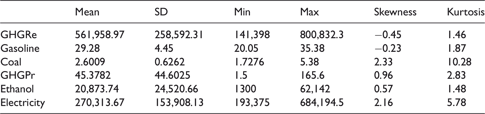
Gasoline: gasoline prices; Coal: coal prices; GHG: greenhouse gas; GHGPr: GHG prices; Ethanol: ethanol production; Electricity: electricity generation; GHGRe: GHG reduction; SD: standard deviation.

Stationary test

As time series data are being used, it is necessary to examine the stationarity properties of the data. In this study, we employ the conventional augmented Dickey–Fuller (ADF) and Phillips–Perron (PP) tests. To remove seasonality and mitigate volatility, we first adjust the seasonality of data and then the logarithm is taken on the season adjusted ones. The results of unit root tests are presented in Table 2. The statistics for both tests confirm that the data’s logarithm is weakly stationary.

Table 2.

Test statistics for stationarity analysis.^a

	Ln(Gasoline)	Ln(Coal)	Ln(GHGPr)	Ln(Ethanol)	Ln(Electricity)	Ln(GHGRe)
ADF	−2.99**	−4.15***	−4.13**	−4.73***	−4.39***	−4.47***
PP	−3.02**	−3.06**	−4.13**	−4.73***	−4.64***	−4.47***

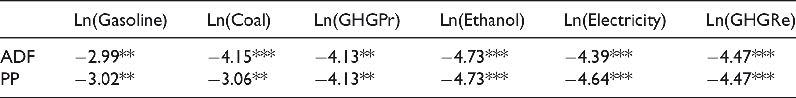
Gasoline: gasoline prices; Coal: coal prices; GHG: greenhouse gas; GHGPr: GHG prices; Ethanol: ethanol production; Electricity: electricity generation; GHGRe: GHG reduction; SD: standard deviation.

^aThe null hypothesis of the tests is that the variable is non-stationary. *** and ** denote significance at 1% and 5% respectively.

Validity analysis of the instrumental variables

To analyze the validity of the instrumental variables, this study makes use of the conventional endogeneity test and the consistent significance test of Racine et al.⁴⁵ and Racine.⁴⁶

First, this study implements the tests proposed by Durbin,⁴⁷ Wu,⁴⁸ and Hausman⁴⁹ to verify the potential endogeneity of ethanol production and electricity generation. In the tests, this study uses the lagged terms of ethanol production and electricity generation as the instrumental variables. The results in Table 3 show that the null hypothesis of exogeneity is rejected in both tests at a 5% significance level. In other words, ethanol production and electricity generation are endogenous.

Table 3.

Endogeneity test.^a

Durbin's chi-squared statistics	Wu–Hausman F statistic
6.43**	3.53**
(0.04)	(0.04)

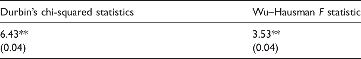
^aThe null hypothesis of the test is that the variable is exogenous. Numbers in parentheses are p values. ** denotes significance at 5%.

Second, this study employs a consistent test of significance of instrumental variables in a first-stage kernel regression to verify whether the instrumental variables are correlated with the endogenous covariates. The test is based on Racine et al.⁴⁵ and Racine⁴⁶.^d The results in Table 4 demonstrate that the lagged ethanol production and the lagged electricity production are significant in the first-stage kernel regressions (i.e. equation (1) and (2), respectively. Therefore, the instrumental variables used are correlated with the endogenous covariates, which implies the validity of the instrumental variables.

Table 4.

Significance test of instrumental variables.^a

Equation of ethanol production	Equation of electricity production
0.05***	0.02**
(0.01)	(0.03)

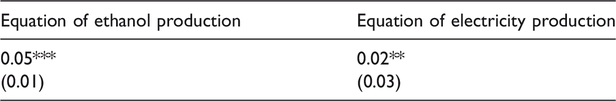
^aThe null hypothesis of the test is that the instrumental variable is not significant. Reported numbers are bandwidths and the associated p values (in parentheses). *** and ** denote significance at 1% and 5% respectively.

Specification error test

In addition to the endogeneity problem, model misspecification could result in a biased estimation. One possible misspecification problem in the linear model comes from the nonlinear combination of exogenous variables. Therefore, this study employs the Ramsey⁵⁰ RESET test to verify the linear specification of the regression model. In the test, the artificial model is given by

Y = X β + \sum_{i = 2}^{p} {\hat{Y}}^{i} γ_{i} + ε

(6)

where $Y$ is the reduction of GHG emissions, and $X$ includes gasoline prices, coal prices, GHG prices, predicted ethanol production, predicted electricity generation, and lagged reduction of GHG emissions. $\hat{Y}$ is the fitted values of $Y$ . This study tests whether $γ_{2} = γ_{3} = γ_{4} = 0$ when $p = 4$ . The F test statistic is 0.68 and the p value is 0.5109.^e Therefore, the linear model in this study is supported.

Test for the significance of dynamics in the second-stage regression

The lagged reduction of GHG emissions is added in the second-stage estimation to mitigate potential serial correlation. This study implements two serial correlation tests, Durbin and Watson⁵¹ and Breusch and Godfrey,⁵² to verify whether the lagged reduction of GHG emissions is useful in the second-stage regression. In Table 5, the results of the Durbin–Watson tests demonstrate that the regression has a positive serial correlation without the lagged reduction of GHG emissions. However, there is no evidence from the Durbin–Watson statistics to show that adding the lagged reduction of GHG emissions can help mitigate serial correlation. On the other hand, the Breusch–Godfrey test shows that the covariate (lagged reduction of GHG emissions) is able to reduce the serial correlation occurring in the second-stage regression. Considering the results of the two tests, this study treats the lagged reduction of GHG emissions as a covariate in the second-stage regression to reduce potential serial correlation.

Table 5.

Test statistics for serial correlation.^a

Without lagged GHG reduction		With lagged GHG reduction
Durbin–Watson	Breusch–Godfrey	Durbin–Watson	Breusch–Godfrey
1.08	9.23***	1.57	1.93
[1.33,1.72]	(0.002)	(1.27,1.78)	(0.16)

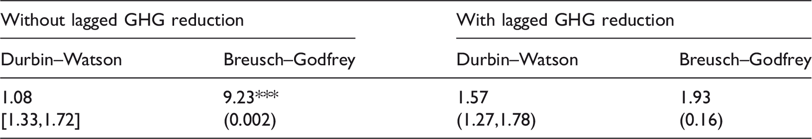
GHG: greenhouse gas.

^aNumbers in brackets are critical values at 5% significance. Numbers in parentheses are p values. *** denotes significance at 1%.

Two-stage semi-parametric dynamic regression analysis

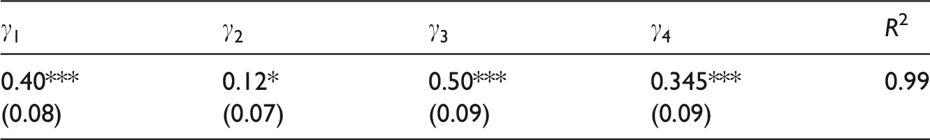
Based on the results of previous statistical tests, this section demonstrates the estimation of the two-stage dynamic semi-parametric model. The robust estimated results for the second-stage dynamic regression (equation (10)) are reported in Table 6.^f The results denote that GHG prices have a significant positive impact on the reduction of GHG emissions at a 1% significance level. This result is not surprising considering that, as the costs of GHG emissions increase with GHG prices, a positive relationship between the reduction of GHG emissions and GHG prices is expected. Moreover, the reduction of GHG emissions increases by 0.41% when GHG prices increase by 1%. On the other hand, the relationships between the reduction of GHG emissions and coal prices and between the reduction of GHG emissions and gasoline prices are found to be insignificant. This may be because coal and gasoline prices do not have a direct impact on the reduction of GHG emissions.^g Meanwhile, electricity generation is found to have a positive impact on the reduction of GHG emissions. As electricity generation increases by 1%, the reduction of GHG emissions increases by approximately 0.48%. At the same time, the relationship between ethanol production and the reduction of GHG emissions is insignificant. These results imply that controlling electricity production, rather than ethanol production, may be a useful method of reducing GHG emissions.

Table 6.

Estimation of second-stage dynamic regression.^a

$β_{1}$	$β_{2}$	$β_{3}$	$β_{4}$	$β_{5}$	$β_{6}$	R ²
0.12	−0.06	0.41***	0.11	0.48***	0.35***	0.99
(0.41)	(0.22)	(0.08)	(0.07)	(0.10)	(0.10)

^aNumbers in parentheses are standard errors. *** denotes significance at 1%.

Based on our estimation results, the transmission mechanism between coal and gasoline prices and the reduction of GHG emissions is described in Figure 1. It can be observed that ethanol and electricity generation have a direct influence on reducing GHG emissions. The mechanism by which the prices of gasoline (coal) influence GHG emissions is through the demand of substitutes such as ethanol (electricity).

Figure 1.

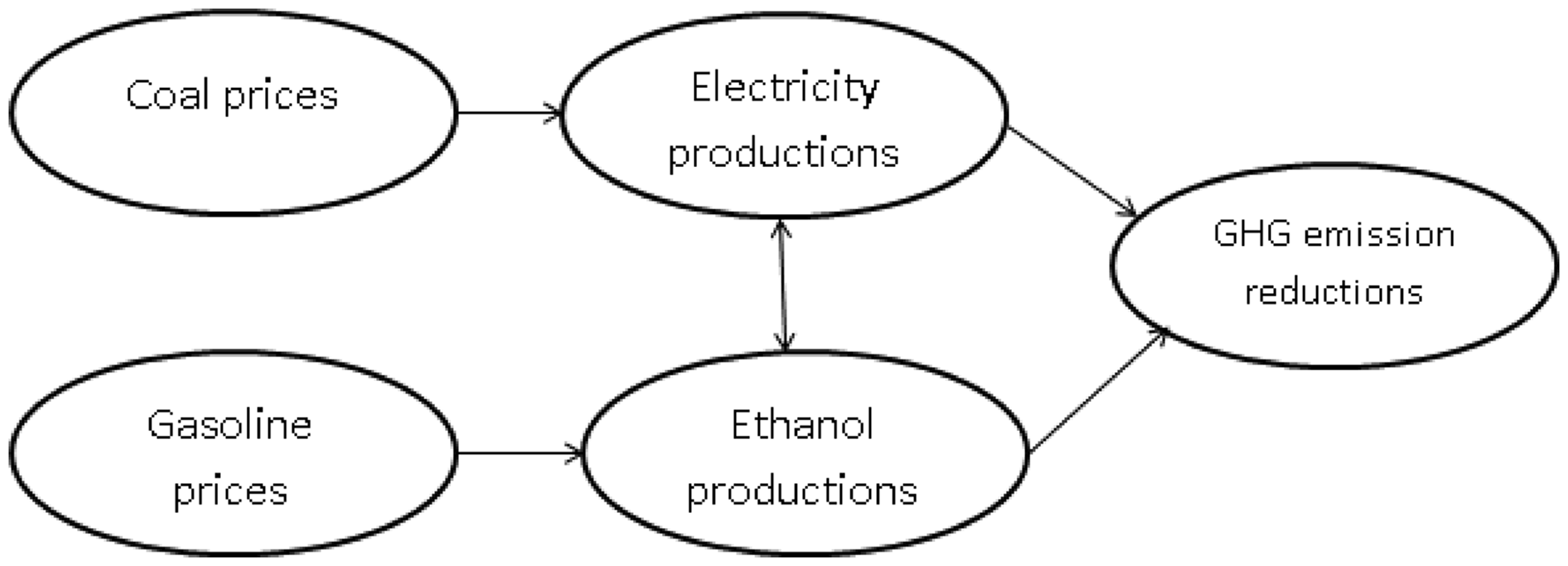
The transmission mechanism of coal and gasoline prices.

Robust analysis of the two-stage dynamic semi-parametric model

In the previous section, it is observed that the effects of coal and gasoline prices on the reduction of GHG emissions are indirect and effected through ethanol and electricity generation. In other words, coal and gasoline prices have no direct impact on the reduction of GHG emissions given a certain level of ethanol production and electricity generation. In this section, we test whether there are significant changes if coal and gasoline prices are treated as the instrumental variables. The first-stage models follow equations (6) and (7), whereas the alternative second-stage regression is given by

{GHGRe}_{t} = γ_{1} {GHGPr}_{t} + γ_{2} {\hat{Ethanol}}_{t} + γ_{3} {\hat{Electricity}}_{t} + γ_{4} {GHGRe}_{t - 1} + ϵ_{t}

(7)

The results, reported in Table 7, demonstrate that the estimated parameters of each covariate are broadly consistent with the results in Table 6, denoting the goodness of fit of the proposed two-stage dynamic semi-parametric model.

Table 7.

Estimation of alternative second-stage dynamic regression.^a

$γ_{1}$	$γ_{2}$	$γ_{3}$	$γ_{4}$	R ²
0.40***	0.12*	0.50***	0.345***	0.99
(0.08)	(0.07)	(0.09)	(0.09)

^aNumbers in parentheses are standard errors. *** and * denote significance at 1% and 10%, respectively.

Discussion

Prior to the Legislation of the Renewable Energy Development Act, which was approved in 2009 and provided a comprehensive regulatory framework for bioenergy, bioenergy production in the forms of electricity generation and liquid fuels had been promoted with the financial support of the Air Pollution Control Fund and the Petroleum Fund.^53,41 In view of this promotion of bioenergy, however, the reduction of GHG emissions for a given level of bioenergy use has declined from 2008 (see Figure 2), indicating that the GHG emissions mitigation capacity of using bioenergy has been reduced. Moreover, bioenergy’s share of total renewable energy approximates only 21.31%. These observations indicate that bioenergy has much room for development in Taiwan. Our simulation results indicate that bioelectricity can generate 2.72 billion kWh annually from utilizing idle land. If bioelectricity is appropriately combined with other renewable technologies, net electricity generation will be much higher, which is beneficial both for the domestic energy supply and for reducing GHG emissions.

Figure 2.

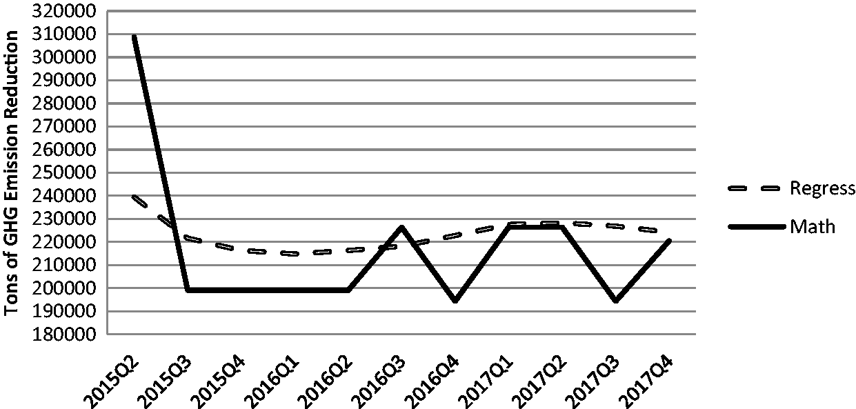
Forecasted GHG reduction based on proposed model (Regress) and mathematical optimization (Math). GHG: greenhouse gas.

The possible reasons that bioelectricity should be incorporated and encouraged are twofold: first, our results show that controlling GHG prices and electricity generation are effective approaches to reducing GHG emissions, implying that the effectiveness of an emissions limits policy is strongly related to the GHG trading market and coal prices; second, with limited land available for energy crop production, ethanol production that fulfills transportation needs will reduce the use of more mitigation effective technology, such as bioelectricity. Therefore, to slow down net GHG emissions, policies should first aim at the production of bioelectricity instead of liquid biofuels such as ethanol or biodiesel.

Potential ways to achieve this goal include but are not limited to:

Incentive to farmers: our study shows that given the current prices of coal, gasoline and GHG emissions, less than half of released land is used to produce energy crops. This may result from the high marginal cost of producing energy crops on less productive land and lack of farmer participation. Therefore, the government may need to determine the appropriate amount of subsidies to farmers such that more land can be engaged in bioenergy production. However, this strategy may be very costly because the subsidy would be paid to all farmers. Farmers who previously participated with lower payments would also enjoy the more generous payments.

Incentive to electricity producers: unlike gasoline, which is supplied by dispersed producers, a large share of electricity is provided by the National Taiwan Power Corporation, which is owned by the Taiwanese government. Executive officers of power plants do not have enough incentive to generate more bioelectricity under current policies. If the government provided certain incentives to existing electricity producers and reduced entry barriers, at high GHG prices more bioelectricity might be produced and more GHG emissions would be sequestered.

Emissions trading system: our results show that bioelectricity is a more effective approach to offsetting GHG emissions than ethanol. However, one of the possible reasons that bioelectricity is not emphasized by the market is that Taiwan does not have an emissions trading system to realize the monetary benefits of the reduction of GHG emissions from bioenergy production. The high emissions offset potential of bioelectricity is neglected due to the lack of an appropriate emissions trading system. Establishing a market for bioenergy producers to realize such gains may encourage the development of bioelectricity.

Forecasting of the reduction of GHG emissions

Because emissions induced climate change has long-term impacts, it is important to know the potential future patterns of GHG emissions that directly influence climate change. Therefore, our study is extended to forecast the reduction of GHG emissions in terms of the proposed model. To verify forecasting accuracy, this study evaluates the out-of-sample performance of the proposed model in terms of the MFE and MAPE. To fulfill the requirements of the forecasting model, this study uses an autoregressive-moving-average model (ARMA) model to forecast the gasoline and coal price series.^h Finally, the reduction of GHG emissions forecasts are reported.

Forecasting accuracy for the reduction of GHG emissions

In “Methodology” section, a two-stage dynamic semi-parametric regression model is shown to be sufficient to estimate the relationship between the reduction of GHG emissions and bioenergy. However, whether this model is able to provide convincing forecasting accuracy is still unknown. This study evaluates the out-of-sample performance of the proposed model. MFE and MAPE are the criteria used to determine forecasting performance. This study divides the whole sample into two subgroups: from fourth quarter 2003 to fourth quarter 2012 (group 1) and from first quarter 2013 to first quarter 2015 (group 2). Group 1 is used for in-sample model estimation, whereas group 2 is used for out-of-sample model validation.

The steps to evaluate the out-of-sample performance of a model are as follows.

Estimate the coefficients associated with the data of group 1 in terms of the proposed model.

Predict the reduction of GHG emissions for the first period of group 2 based on the estimates in (A). Then, compute the forecasting errors (FE) and the absolute percentage errors (APE) between the predicted and actual reduction of GHG emissions for the first period of group 2 by

{FE}_{1} = (Y_{1} - {\hat{Y}}_{1}) and {APE}_{1} = 100 \times \frac{| Y_{1} - {\hat{Y}}_{1} |}{Y_{1}}

(8)

Estimate the coefficients associated with the model by using the data of group 1 and the first period of group 2.

Predict the reduction of GHG emissions for the second period of group 2. Then, compute the FE and APE between the predicted and actual reduction of GHG emissions for the second period of group 2 by

{FE}_{2} = (Y_{2} - {\hat{Y}}_{2}) and {APE}_{2} = 100 \times \frac{| Y_{2} - {\hat{Y}}_{2} |}{Y_{2}}

(9)

Continue (C) and (D) until all forecasting squared errors linked to group 2 are evaluated.

From the results in Table 8, it can be observed that MFE and MAPE are 0.0780 and 0.95%, respectively. The values of MFE imply that the proposed two-stage dynamic semi-parametric model tends to under-forecast the reduction of GHG emissions, which is not a critical problem as under-forecasted reductions of GHG emissions can encourage the government to make more efforts to achieve the intended reduction of GHG emissions target. Meanwhile, the value of MAPE is less than 1%, revealing a convincing forecasting performance of the proposed model.

Table 8.

Evaluation of out-of-sample performance.^a

	2013Q1	2013Q2	2013Q3	2013Q4	2014Q1	2014Q2	2014Q3	2014W4	2015Q1	Average
Y	12.33	12.20	12.33	12.33	12.33	12.33	12.20	12.33	12.69	12.34
${\hat{Y}}_{2 sls}$	12.06	12.28	12.23	12.29	12.29	12.30	12.30	12.25	12.37	12.26
FE	0.27	−0.08	0.09	0.04	0.04	0.03	−0.09	0.0774	0.32	0.08
APE	2.18	0.68	0.81	0.36	0.36	0.20	0.81	0.63	2.56	0.95

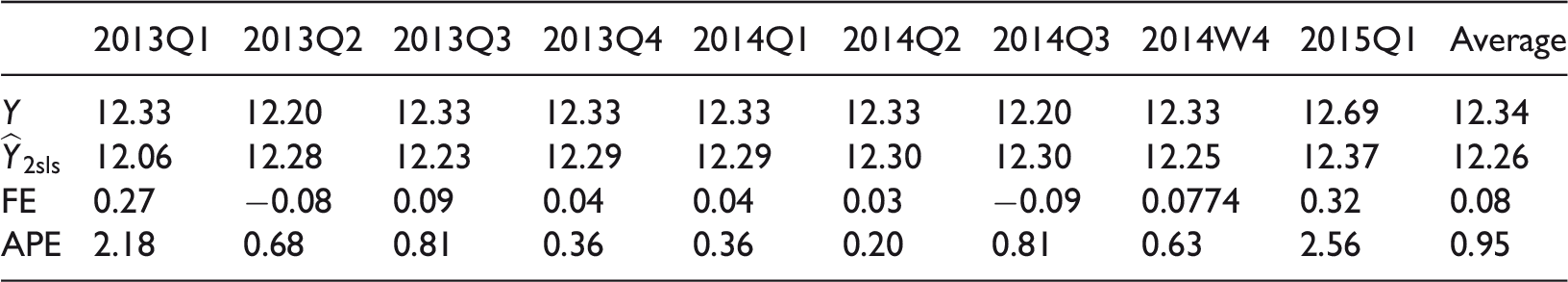
^aThe numbers (taking logarithm) in the first and second denote the actual GHG reduction and predicted GHG reduction by the proposed model, respectively. The last two lines denote the forecasting errors (FE) and absolute percentage errors (APE), respectively.

Prediction of gasoline and coal prices

As gasoline prices, coal prices, GHG prices, ethanol production, electricity generation, and the reduction of GHG emissions after the first quarter of, 2015 are still unknown, we need to predict three prices and evaluate the corresponding level of ethanol production, electricity generation, and the reduction of GHG emissions using optimization models. This study uses an ARMA to predict the gasoline and coal price series with a one-step-ahead approach.

The ARMA model has the structure

Z_{t} + a_{1} Z_{t - 1} + \dots + a_{p} Z_{t - p} = c_{1} e_{t - 1} + \dots + c_{q} e_{t - q} + e_{t}

(10)

where $Z_{t}$ is the output at time t, $e_{t}$ is the white noise disturbance, and p and $q$ stand for the orders of $Z_{t}$ and $e_{t}$ . It can be written as

A (L) Z_{t} = C (L) e_{t}

(11)

where $A (L) = 1 + a_{1} L + \dots + a_{p} L^{p}$ , $C (L) = 1 + c_{1} L + \dots + c_{q} L^{q}$ , and $L$ is the lag operator. In our study, the mean square error is the criterion used to select the optimal number of lags.

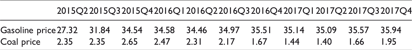
Predicted gasoline and coal prices from the second quarter of 2015 to the fourth quarter of 2017 are listed in Table 9.

Table 9.

Prediction of gasoline and coal prices.

	2015Q2	2015Q3	2015Q4	2016Q1	2016Q2	2016Q3	2016Q4	2017Q1	2017Q2	2017Q3	2017Q4
Gasoline price	27.32	31.84	34.54	34.58	34.46	34.97	35.51	35.14	35.09	35.57	35.94
Coal price	2.35	2.35	2.65	2.47	2.31	2.17	1.67	1.44	1.40	1.66	1.95

GHG prices after the first quarter of 2015 are assumed to be the same as those in the first quarter of 2015 because these prices remain consistent after 2013. We further use mathematical optimization to evaluate corresponding electricity generation and ethanol production.ⁱ

Forecasting of the reduction of GHG emissions

In this section, we forecast the reduction of GHG emissions by means of the proposed model. The forecasting periods cover from the second quarter of 2015 to the fourth quarter of 2017. The N-step-ahead approach is adopted in the study where $N = 1, \dots, 11$ . The logic of N-step-ahead forecasting is that the benefit in terms of regression is similar to that of out-of-sample evaluation. In addition, we use a mathematical programming model to predict the reduction of GHG emissions. The results are reported in Figure 2.

The minimum and maximum forecasted reductions of GHG emissions based on the proposed model are of 214,806 and 239,497 tons, respectively. The reductions of GHG emissions forecasted by the mathematical model vary between 194,359 and 308,766 tons. The average reduction of GHG emissions forecasted by the proposed model is of 223,331 tons, whereas that forecasted by the mathematical model is of 217,580 tons. The volatility of reduction of GHG emissions forecasted by the proposed model is lower than that forecasted by the mathematical optimization model.

In the first quarter of 2015, the reduction of GHG emissions forecasted by the proposed model is much smaller than that evaluated by the mathematical approach. After the second quarter of 2015, the reduction of GHG emissions forecasted by the two methods become closer. The average percentage error^j is 4.21%, implying the proposed model is capable of replacing the mathematical optimization approach in terms of forecasting the reduction of GHG emissions. That is, if data on gasoline prices, coal prices, GHG prices, ethanol production, and electricity generation are available, the two-stage dynamic semi-parametric regression is an appealing model to forecast the reduction of GHG emissions.

Concluding remarks

GHG emissions are a critical source of climate change. Methods such as tax (subsidy) policy and legislation are potential tools for the government to mitigate GHG emissions. Instead of probing the policy effect, this study investigates how the reduction of GHG emissions can be influenced by ethanol production and electricity generation, and by relevant economic factors such as gasoline prices, coal prices, and GHG prices.

Some of our estimation results are consistent with the literature. First, the GHG price has a significant positive impact on reducing GHG emissions, whereas coal and gasoline prices have no such direct impact. Second, the stimulation of ethanol production does not work to reduce GHG emissions. In contrast to findings in Murray et al.,⁷ this study, however, discovers that bioelectricity can provide a significant contribution to reducing GHG emissions. As electricity generation increases by 1%, the reduction of GHG emissions increases by 0.48%. These outcomes suggest that the Taiwanese government could shift policy support from biofuel production to bioelectricity production to reduce GHG emissions.

This study also forecasts the reduction of GHG emissions from the second quarter of 2015 to the fourth quarter of 2017. The reduction of GHG emissions forecasts vary between 214,806 and 239,497 tons, i.e. less than 3% of projected GHG emissions. In contrast to the complex mathematical programming model, our econometric model provides a parsimonious approach with convincing accuracy to forecast the reduction of GHG emissions. In other words, government analysts should be able to use our model to evaluate emissions reductions given a certain level of bioenergy production and market prices.

Even though many studies have examined the relationship between bioenergy and GHG emissions, they neither distinguish between biofuel and bioelectricity, nor do they estimate the marginal effect of biofuel (or bioelectricity) on GHG emissions. Therefore, the application of our model to other countries may be a subject of interest for future study.

Footnotes

Acknowledgement

We thank the assistance of Dr Wei Huang from National University of Singapore.

Declaration of conflicting interests

The author(s) declared no potential conflicts of interest with respect to the research, authorship, and/or publication of this article.

Funding

The author(s) disclosed receipt of the following financial support for the research, authorship, and/or publication of this article: China Postdoctoral Science Foundation (2016M602078), Distinguished Young Scholar of Jiangxi (20171BCB23047), Scientific Project of Jiangxi’s Department of Education (GJJ160437), University Social Science Foundation of Jiangxi (JC17205), and National Natural Science Foundation of China (71663022; 71663024; 71663025; 71673123).

Notes

Meng-Shiuh Chang received his PhD in Texas A&M University in 2011. He was an assistant professor in Southwest University of Finance & Economics during 2011-2015, associate professor of Jiangxi University of Finance and Econimics during 2015-2017, and is currently a professor of School of Economics at Hubei University. His research interests include econometric analysis and data estimation.

Chih-Chun Kung received his PhD in Texas A&M University in 2010 and is currently a professor of Institute of Ecological Economics at Jiangxi University of Finance & Economics. His research interests include climate change, carbon sequestration, and bioenergy development.

References

Schneider

and McCarl

BA.

Economic potential of biomass based fuels for greenhouse gas emission mitigation. Environ Resour Econ 2003; 24: 291–312.

Haberla

Sprinz

Desaubies

et al . Correcting a fundamental error in greenhouse gas accounting related to bioenergy. Energy Policy 2012; 45: 18–23.

Gelfand

Terenzio

Poonam

et al . Carbon Debt of Conservation Reserve Program (CRP) grasslands converted to bioenergy production. Proc Natl Acad Sci 2011; 108: 13864–13869.

Wang

Well-to-wheels energy and greenhouse gas emission results of fuel ethanol. Lemont, IL: Argonne National Laboratory, 2007.

Yacobucci

and Bracmort

Calculation of lifecycle greenhouse gas emissions for the renewable fuel standard (RFS). Washington, DC: Congressional Research Service, 2010.

Murray

Maureen

Francisco

et al . How effective are US renewable energy subsidies in cutting greenhouse gases? Am Econ Rev 2014; 104: 569–574.

Ozturk

Utilizing biofuels for sustainable development in the panel of 17 developed and developing countries. GCB Bioenergy 2016; 4: 826.

Tso

and Su

Domestic bio-ethanol sources productivity and energy and economic indicators research. Taiwan J Agric Econ 2009; 30: 47–64.

Chen

McCarl

Chang

et al . Evaluation the potential economic impacts of Taiwanese biomass energy production. J Biomass Bioenergy 2011; 35: 1693–1701.

10.

Intergovernmental Panel on Climate Change. In: Watson RT, Zinyowera MC and Moss RH (eds) Climate change 1995: impacts, adaptations and mitigation of climate change: scientific-technical analysis. Cambridge: Cambridge University Press, 1995, p.879.

11.

Pastor

and Post

WM.

Response of northern forests to COR₂R-induced climate change. Nature 1988; 334: 55–58.

12.

Rosenzweig

and Parry

ML.

Potential impact of climate change on world food supply. Nature 1994; 367: 133–138.

13.

Fussel

HM.

Adaptation planning for climate change: concepts, assessment approaches, and key lessons. Sustain Sci 2007; 2: 265–275.

14.

Metz

Davidson

Swart

et al . Climate change mitigation. The working group III contribution to the IPCC third assessment report, 2001.

15.

Mendelsohn

and Neumann

JE.

The impact of climate change on the United States economy. Cambridge, UK: Cambridge University Press, 1999, 344 pp.

16.

Reilly

JM.

Agriculture: the potential consequences of climate variability and change for the united states. Cambridge, UK: Cambridge University Press, 2002, 136 pp.

17.

Liu

and Cirillo

A model system to evaluate the impacts of vehicle purchase tax and fuel tax on household greenhouse gas emissions. In: 94th annual meeting of the Transportation Research Board, Washington, DC, 11–15 January 2015.

18.

Paleti

Bhat

Pendyaia

et al . Assessing the impact of transportation policies on fuel consumption and greenhouse gas emissions using a household vehicle fleet simulator. J Transport Res Board 2014; 2: 182–190.

19.

and Lin

Factors affecting carbon dioxide (COR₂R) emissions in China's transport sector: a dynamic nonparametric additive regression model. J Cleaner Prod 2015; 101: 311–322.

20.

Anjum

Burke

Gerlagh

et al . Modeling the emissions-income relationship using long-run growth rates, CCEP. Working Papers #1403, 2014.

21.

Brännlund

Karimu

and Söderholm

Convergence in carbon dioxide emissions and the role of growth and institutions: a parametric and nonparametric analysis. CERE Working Paper, 2014.

22.

Sanchez L and Stern

DI.

Drivers of industrial and non-industrial greenhouse gas emissions. Centre for Climate Economic & Policy. Working paper, 2015.

23.

Chakir

Cara

and Vermont

Price-induced changes in greenhouse gas emissions from agriculture, forestry, and other land use: a spatial panel econometric analysis. EAAE 2014 Congress, Ljubljana, Slovenia, 26–29 August.

24.

De Cara

and Jayet

PA.

Marginal abatement costs of greenhouse gas emissions from European agriculture, cost-effectiveness, and the EU non-ETS burden sharing agreement. Ecol Econ 2011; 70: 1680–1690.

25.

Hoel

and Sletten

TM.

Climate and forests: the tradeoff between forests as a source for producing bioenergy and as a carbon sink. Resour Energy Econ 2016; 43: 112–129.

26.

Molinos-Senante

Hernandez-Sancho

Mocholi-Arce

et al . Economic and environmental performance of wastewater treatment plants: potential reductions in greenhouse gases emissions. Resour Energy Econ 2014; 38: 125–140.

27.

Tsurumi

and Managi

The effect of trade openness on deforestation: empirical analysis for 142 countries. Environ Econ Policy Stud 2014; 16: 305–324.

28.

Arvizu

Biofuels: too soon to give up. Science 2008; 320: 1419–1420.

29.

Fargione

Hill

Tilman

et al . Land clearing and the biofuel carbon debt. Science 2008; 319: 1235–1238.

30.

Lehmann

A handful of carbon. Nature 2007; 447: 143–144.

31.

McCarl

BA.

Food, biofuel, global agriculture, and environment: discussion. Rev Agric Econ 2008; 30: 530–532.

32.

McCarl

Peacocke

Chrisman

et al . Economics of biochar production, utilization, and GHG offsets. In: Lehmann

and Joseph

(eds) Biochar for environmental management: science and technology. London: Earthscan Publisher, 2009, pp.341–357.

33.

Searchinger

Heimlich

Houghton

et al . Use of U.S. croplands for biofuels increases greenhouse gases through emissions from land-use change. Science 2008; 319: 1238–1240.

34.

Petersen

Haigh

and Görgens

JF.

Techno-economics of integrating bioethanol production from spent sulfite liquor for reduction of greenhouse gas emissions from sulfite pulping mills. Biotechnol Biofuels 2014; 7: 169–182.

35.

Campiche

Bryant

and Richardson

JW.

Long-run effects of falling cellulosic ethanol production costs on the US agricultural economy. Environ Res Lett 2010; 5: 14–18.

36.

Kim

Peralta

and McCarl

BA.

Land-based greenhouse gas emission offset and leakage discounting. Ecol Econ 2014; 105: 265–273.

37.

McCarl

and Schneider

UA.

Agriculture’s role in a greenhouse gas emission mitigation world: an economic perspective. Rev Agric Econ 2000; 22: 134–159.

38.

Shie

Tsou

Lin

et al . Bioenergy and products from thermal pyrolysis of rice straw using plasma torch. Bioresour Technol 2010; 101: 761–768.

39.

Tsai

WT.

Potential analysis of common crop residues for bioenergy sources in Taiwan. Energy Sources B Econ PlannPolicy 2014; 9: 32–38.

40.

Tsai

Lin

and Yeh

CW.

An analysis of biodiesel fuel from waste edible oil in Taiwan. Renew Sustain Energy Rev 2007; 11: 838–857.

41.

Chang

CC.

The potential impacts of climate change on Taiwan’s agriculture. Agric Econ 2002; 27: 51–64.

42.

Chen

and Chang

CC.

The impact of weather on crop yield distribution in Taiwan: some new evidence from panel data models and implications for crop insurance.

J Agric Econ 2005; 33: 503–511.

43.

Kung

McCarl

Chen

et al . Environmental impact and bioenergy production from pyrolysis in Taiwan. Energy Environ 2014; 25: 13–39.

44.

and Racine

JS.

Nonparametric econometrics: theory and practice. Princeton: Princeton University Press, 2007.

45.

Racine

Hart

and Li

Testing the significance of categorical predictor variables in nonparametric regression models. Econometr Rev 2006; 25: 523–544.

46.

Racine

JS.

Consistent significance testing for nonparametric regression. J Business Econ Stat 1997; 15: 369–379.

47.

Durbin

(1954) Errors in variables. Rev Int Stat Inst 1954; 22: 2332.

48.

DM.

Alternative tests of independence between stochastic regressors and disturbances. Econometrica 1973; 41: 733–750.

49.

Hausman

JA.

Specification tests in econometrics. Econometrica 1978; 46: 1251–1271.

50.

Ramsey

JB.

Tests for specification errors in classical linear least squares regression analysis. J R Stat Soc B 1969; 31: 350–371.

51.

Durbin

and Watson

GS.

Testing for serial correlation in least squares regression, I. Biometrika 1950; 37: 409–428.

52.

Breusch

and Godfrey . Testing for autocorrelation in dynamic linear models. Aust Econ Papers 1978; 17: 334–355.

53.

Tsai

and Hsien

KJ.

An analysis of cogeneration system utilized as sustainable energy in the industrial sector in Taiwan. Renew Sust Energy Rev 2007; 11: 2104–2120.