
Abstract
The main purpose of this study is to propose a reduction of inventory based on non-industrial sectors reflecting the characteristics of local governments and efficient greenhouse gas reduction activities in Korea. Although national government has implemented various policies and systems to reduce greenhouse gas emissions, it would only remain in industrial and public areas. Thus, in order to reduce national greenhouse gas emissions, local governments should play a major role as a leading management entity and it is necessary to adopt efficient and systematic management of the non-industrial sector, which accounted for a significant portion of the country’s emissions. However, the policy of the local governments to reduce greenhouse gas emissions has not been effective due to lacking in connectivity to the central government’s plan or presenting it in a simple listing format. The characteristics of inventory building such as main purpose, boundary setting, emission source, policy setting, range, organizing body, relevant law of inventory building between national government, and local governments are quite different from the start. In order to reflect the actual greenhouse gas reduction activities of the local governments, this study reconstructs the categories that are considered to have management authority in the local governments such as home, commercial, and road transportation among the scope 1 of the local governments inventory and scope 2 for establishing effective policies to reduce greenhouse gas emissions in local governments. This study also proposes reduced inventory by reorganizing categories that local governments deem to have managerial authority among direct and indirect emission of greenhouse gas inventory.
Keywords
Introduction
With the Paris Agreement, the basis for the post 2020 new climate regime, the response trend to the global climate change has shifted from some developed countries to a universal response system involving all countries. 1 While the existing Kyoto Protocol has only required to reduce greenhouse gas (GHG) emissions in 37 countries, the new climate system gave all parties including 197 countries, a duty to reduce GHG emissions. 2 According to the “Roadmap to Achieve the National Reduction Goals for 2030” in Korea, national government is expected to release about 851 million tons CO2eq. by 2030, of which it plans to reduce GHG by 315 million tons, or about 37%. Korea’s total reduction target is 2.19 million tons, with buildings (35.8%), transportation (25.9%), public equipment (3.6%), waste (3.6%), and agricultural and livestock (1%), accounting for about 32% the total reduction target. 3
In the meantime, national government implemented various policies and systems to reduce GHG emissions, but had limitations that would remain only in industrial and public areas, which has adopted target management system and emission trading system. It is necessary to adopt efficient and systematic management of the non-industrial sector, which accounted for a significant portion of the country’s emissions. Accordingly, in order to achieve the national GHG reduction target, continued support for local governments, which are the de facto subject of reduction, will have to be strengthened considering the importance of non-industrial sector management with high potential and capacity is growing.
The Ministry of Environment and the Korea Environment Corporation have calculated and provided GHG emissions from 243 local governments nationwide since 2015 to support voluntary reduction of GHG by local governments. 4 However, since the implementation of the Green Act in 2010, the policy of the local governments to reduce GHG emissions have not been effective due to lacking in connectivity to the central government’s plan or presenting it in a simple listing format. Although the measures for reducing greenhouse gases are being implemented, a cyclical reduction policy system, which evaluates the performance of the reduction measures, and modifies and reflects the results in the reduction plan, is not working properly. Thus, the purpose of building a greenhouse gas inventory for local governments is to use it as basic data for local governments’ reduction policies, such as selecting effective means of reduction and setting reduction targets through analysis of emission characteristics, as well as identifying emission status by local governments. In this regard, this research focused on the existence of local governments’ control and presented highly useful categories by reorganizing the reduction inventory based on direct and indirect emissions, so that local governments could come up with practical measures and induce voluntary reductions in the establishment and implementation of reduction policies. In order to reduce national GHG emissions, local governments should become the leading management entity, and inventory should be built first, including calculating emissions that can be reduced by local governments in consideration of their emission characteristics and rights. Therefore, this study is intended to present a reduction of inventory based on non-industrial sectors reflecting the characteristics of local governments and efficient GHG reduction activities. In particular, this study tries to present a reduced inventory by reorganizing categories that local governments deem to have managerial authority among direct and indirect emission of GHG inventory, such as home, commercial, and road transport sectors.
Data and methods
GHG inventory of local governments was calculated on the basis of five calculation principles: reasonable, completeness, consistency, transparency, and accuracy, reflecting the concept of local governments and single sources of enterprise emissions in the internationally accepted calculation method. 5 The calculation areas, based on 2006 IPCC (Intergovernmental Panel on Climate Change) G/L, were divided into two areas: direct emission (Scope 1) and indirect emission (Scope 2), and direct emission was reclassified into four areas: energy, industrial process, AFOLU, and waste. Indirect emission refers to GHG emissions generated by consumption of goods produced, such as power and heat use and waste generation, and is calculated only by local governments, not by national inventory. In addition, a separate category was reorganized so that local governments’ efforts to reduce GHG emissions could be practically reflected and a reduction event was presented. GHG under inventory are six substances specified in the Kyoto protocol: CO2, CH4, N2O, PFCs, HFCs, and SF6, and GHG emissions are converted to CO2 in consideration of the global warming potential and are shown as an equivalent value (eq.). The tier of the GHG inventory is generally divided into three, from tier 1 to tier 3, based on accuracy and reliability of the emission data and coefficient, meaning the higher the level, the more accurate and reliable the results. For GHG inventory of local governments, tier 1 or tier 2 calculation levels were applied according to categories. In order to reflect the emission characteristics of local governments’ GHG, it is highly accurate to apply emission coefficients of local governments or facilities.
However, it is currently impossible to apply these emission coefficients to all categories calculated. Thus, emission coefficient at the level of local governments or facilities developed in Korea was applied first, and if not possible, national unique emissions coefficient was used. Therefore, this study applied the emission coefficient at the level of local governments or facilities developed in the country first, and, if not possible, national unique emission coefficient or the 2006 IPCC G/L Default was used. 6 Although the principle was to use statistical data published by the government and local governments, the emission was calculated by considering regional characteristics of the activity data published by local governments.
The IPCC published the international guidelines for 1996 IPCC G/L to assess GHG emissions/absorbance by country, and three additional guidelines were subsequently published. The published guidelines include GPG 2000 (good practice guidelines 2000), which supplemented 96 IPCC G/L, GPG-LULUCF (Good Practice Guideline for land use, land-use change, and forest), which adds a method of assessing emissions/capacity in accordance with the Marrakesh agreement, and 2006 IPCC G/L, which has been restructured and supplemented to the published guidelines. 7 Compared to the national inventory calculation standard by 1996 IPCC G/L, the local inventory calculation standard by 2006 IPCC G/L showed the major differences in methodology, calculation category and emission factor defaults. 8 In the energy sector, unlike the 1996 IPCC G/L, 2006 IPCC G/L changed the number of fuel consumption for raw materials, such as lead generation for raw materials in the petroleum industry, to be excluded from the calculation of the energy sector, and the number of categories increased, with the manufacturing sector being subdivided into 13 industries from six industries. In addition, CO2 transport and storage sectors, fuel burn and de-routine emission sectors were added. In the calculation methodology, 1996 IPCC G/L applies the oxidation rate and carbon immersion by fuel in the calculation of the fuel burn sector, and includes the fuel consumption for raw materials in the energy sector, whereas 2006 IPCC G/L assumes full oxidation, and non-energy-supporting fuels are excluded from the calculation of the energy sector emissions. In the industrial process field, the “industrial process and solvent use” section of the 1996 IPCC G/L was integrated into “industrial process and other products use of 2006 IPCC G/L.” In the case of steel production (electricity) emissions, 1996 IPCC G/L is reported in the energy sector, while 2006 IPCC G/L is reported in the industrial process sector. The 2006 IPCC G/L showed different GHG emission coefficients for some categories of industrial processes due to the revision of emission coefficients and the addition of new emission coefficients. The 1996 IPCC G/L comprises the AFOLU sector exclusively for agriculture, forests, and grasslands, while the 2006 IPCC G/L incorporates agriculture and LULUCF section as AFOLU. In addition, unlike the 1996 IPCC G/L, which was assessing biomass accumulation changes for two identifiers (forests, grasslands), the 2006 IPCC G/L targeted six identifiers (forests, farmland, grasslands, wetlands, residential areas, and other lands). In the 2006 IPCC G/L, emission sources were further disaggregated, and the calculation methodologies, emission coefficients, etc. for detail not covered by the 1996 IPCC G/L were changed and added. In the waste sector, biological treatment and surface burning of solid waste were added to the 2006 IPCC G/L. 8
Results and discussion
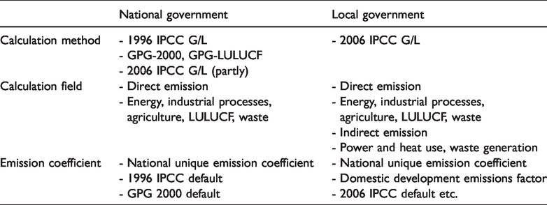
The characteristics of inventory building between national government and local governments are quite different from the start as shown in Table 1.
Comparison of inventory characteristics between national and local government.

The main purpose of the national inventory building is to calculate the total emissions of nation, with most categories being calculated in top-down fashion, but the local government’s inventory building is calculated in bottom-up fashion, reflecting the data, and characteristics of each local government. Local governments have no obligation to report emissions, and they calculate their own emissions to establish policies for coping with climate change. 9 However, national government plans and carries out various reduction policies, including the formal reporting of emissions at home and abroad in accordance with international standards, and the establishment of a basis for its policy on coping with climate change. In addition, local governments are self-calculating emissions within their administrative authority and implementing national government’s reduction policies or conducting activities to reduce GHG emissions of public facilities in local governments. 10 National government only targets direct emission sources due to unnecessary classification of emission boundaries, but local governments distinguish between direct and indirect emission sources because boundary setting is required. National inventory is organized by the GHG General Information Center, and although relevant laws are in place, the inventory construction by local governments is not legally mandatory and is carried out by the government agency.
National inventory was based on the MRV guidelines from the 1996 IPCC G/L, GPG 2000, GPG-LULUCF, and the Kyoto Protocol will apply the 1996 IPCC G/L during the first agreement period (2005–2012) and gradually switch to the 2006 IPCC G/L after 2020. 11 To reflect the latest guidelines, the local governments applied the guidelines developed by agency based on the 2006 IPCC G/L. Different guidelines that are applied to inventory of national and local governments resulted in differences in emission calculation categories and emission coefficients as well as in calculation methodology. The main differences in inventory calculation between the state and local government inventory are as follows in Table 2.
Main differences in inventory calculation between national and local government.
The reason for the different in inventory calculation between national and local governments is that national government calculates emissions for five areas of direct emission, but the local government include four areas of direct emission and indirect emission areas not determined by national government. 12 In calculating methodologies by sector, it was found that in the energy sector, national government includes fuel consumption for raw materials by considering carbon immersion, but local governments include non-energy-supporting fuel in the industrial process area. Further, local governments calculated emissions only by lubricating oil and paraffin wax by using non-energy-assisted fuels in industrial processes, and applied methodologies were different. In the fuel burn sector, local governments calculated their emissions by assuming complete oxidation, but the state applied the oxidation rate by fuel. In AFOLU sector, the national inventory calculation standard consists of “agriculture” of the IPCC G/L and “forestry and grassland only” of the GPG-LULUCF in 1996, but the local government inventory based on the 2006 IPCC G/L has shown that “agriculture” and GPG-LULUCF segments are aggregated into AFOLU.
Because of different calculation criteria applied to inventory of national and local governments, there was a difference between range of categories and default values. For direct emissions, 23 more categories were added to the local government inventory compared to the national inventory, and indirect emissions are calculated only in the local government inventory. The reason why indirect emissions are not considered in the national inventory is that the entire country is considered a single target and production–consumption takes place within one boundary. The number of inventory categories of national and the local government by discipline is shown in Table 3.
Number of inventory categories of national and local government by discipline.

For national government, the system for obtaining activity data is relatively simple, because it is possible to obtain activity data in all areas through affiliated organizations, and it is easy to utilize data such as the GHG target management system statement and only considers import and export statistics. However, local governments use statistical data issued by state agencies, but separately secure data by facility. In some cases, official statistics are used when calculating inventory for countries and local governments, but only national statistics are published. In addition, statistics by local governments are provided, but they do not exist. Therefore, estimates and allocations of activity data are needed to calculate emissions by local governments. The local governments’ inventory uses more detailed activity data than national governments because they utilize not only official statistics but also statistical annals of local governments, various associations and electronic public information systems. In cases where it is difficult to obtain it directly from industrial facilities, the local government applied a method to estimate it by using production capacity and others in Table 4.
Comparison of activity data of national and local government by Sectors.
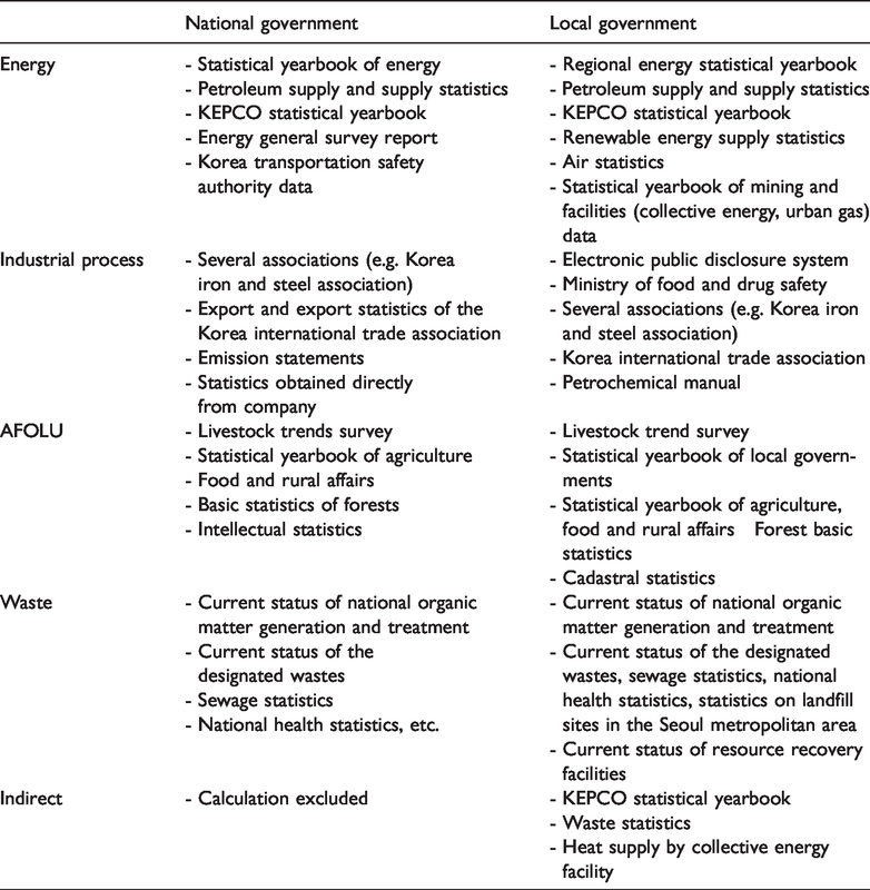
There are some cases where key statistics used by different disciplines are matched, but others are not. In the energy sector, the difference in national emissions occurred because areas where the sea, river, etc. did not exist, even though activity data such as water transport and fishing sectors existed, considering the geographical characteristics of local governments. In the industrial process field, it has been shown that the methodology of the upper tier can be applied since the government can utilize activity data such as the target management system specifications through its affiliated organizations. On the other hand, local governments applied methods to estimated activity data in industrial facilities such as electronic and steel industries. Local governments used official national statistical data such as livestock trends and agriculture statistics yearbook when calculating AFOLU fields, but if there was no national statistics, the statistical yearbooks issued by local governments were used for application of activity data. In the waste sector, the local governments’ inventory was found to be separately collected and used by the facilities, including statistics on landfill sites in the Seoul metropolitan area and the current status of the resource recovery facility operation.
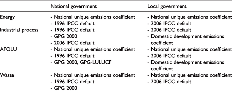
It is difficult to compare and judge the size because the emission coefficient values of national and local governments are different by category and by calculation method. National government applies the new National Oil Emission Coefficient (GIR, 2014) in energy, agriculture (fertile, agricultural soil), LULUCF (forestry), and waste (waste water, incineration) areas, but the local governments apply only the carbon emission coefficient by fuel based on the 2006 heat generation rate among the national high oil emission coefficients. Emission coefficients by sector is shown in Table 5 and the comparison of emission coefficient in energy sector is provided in Table 6 as follows.
Emission coefficients by sector.
Comparison of emission coefficients in energy sector.
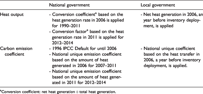
aConversion coefficient: net heat generation ÷ total heat generation.
It was shown that in the energy sector, differences exist in the application of heat generation and carbon emission coefficients of the country’s indigenous oil according to the period of inventory build-up. The purpose of establishing an inventory of local governments’ GHG emissions is not only to identify the current status of each local government’s emissions, but also to use it as a basic data for their reduction policies, such as selecting effective means of reduction and setting targets through analysis of emission characteristics. 13 Local governments are making efforts to establish and implement their own reduction targets, but there are technical limitations in managing the performance of reductions already established and implemented. 14 In addition, due to a lack of budget and expertise, it is difficult to build its own inventory. Therefore, although GHG reduction measures are being implemented, the policy system for cyclical reduction has not been properly implemented, including evaluation of performance of reduction means and revision of plans through reflection of results, due to lack of inventory establishment. 15 Therefore, we present a highly available category by reorganizing the reduction environment based on direct and indirect emission with a focus on the existence of administrative authority of local governments, thereby contributing to voluntary reduction by devising practical measures for the establishment and implementation of reduction policies of local governments. The GHG inventory is used by local governments as basic data for reduction plans, but it is limited to determine the performance of local governments on their reduction activities. Among the GHG emission sources located in local governments, the proportion of GHGs emitted from the industrial facilities and power generation facilities such as steel and electronics industries is quite high, but there is a limit to induce reduction by establishing reduction policies for these categories. In this study, a reduction environment consisting of non-industrial sectors was presented separately, with an emphasis on the presence of local governments’ management authority to reflect their efforts to reduce GHG emissions. The reduced inventory has been reorganized from the overall inventory (direct, indirect discharge) to categories that are considered to have administrative authority, excluding categories not managed by local governments (power plants, airports, industrial facilities, etc.), and mainly non-industrial sectors. Table 7 shows the overall structure of reduced inventory by dividing it into energy and non-energy sectors.
Categories composed of reduced inventory.
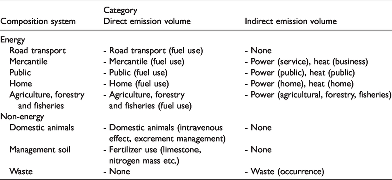
The reduced inventory consisted of categories such as road transport of direct emissions, use of fuel in households, commerce, and the public sector, and power and heat during indirect emissions, and waste generation. The total amount of emissions from 17 local governments nationwide increased steadily since 2005 and then increased and decreased slightly from 2010, and decreased in 2014. The total amount of emissions from the 17 metropolitan areas increased by about 9% during the calculation period from about 255 million tons of CO2eq in 2005 to about 278 million tons of CO2eq in 2014. The reason why emissions from reduced inventory have been on the decline since 2013 is due to the stabilization of carbon point system and green card system, and the expansion of GHG reduction policy activities such as a campaign to reduce GHG emissions by one ton. Table 8 shows reduced inventory by section during the period from 2005 to 2014.
Reduced inventory by section (2005–2014).
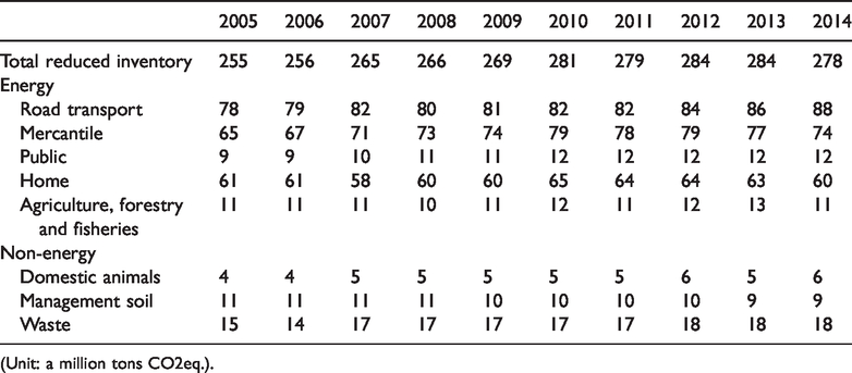
(Unit: a million tons CO2eq.).
The analysis of the emission status of the sector-by-sector reduced inventory showed that the public (31.7%), commercial (13.6%), road transport (13%), and agricultural, forestry, and fisheries (0.4%) increased in 2014 compared to 2005, while the household sector (2.4%) decreased. The proportion of emissions by road transport, commercial and household sectors accounted for about 80% of the total energy sector emissions, of which the road transport sector continued to increase during the calculation period, with the largest proportion of emissions. Emissions from commercial and household sectors have steadily increased during the calculation period and have been declining since 2013. It was found that commercial, public, and household governments had the greatest impact on GHG emissions from power and heat use. Analysis of local governments’ GHG emission trends during the calculation period showed an increase in emissions from power use, but a decrease in GHG emissions from the use of fossil fuels. The share of emissions in the non-energy sector increased from 2005 to 2014 with 33.9% for livestock and 22.7% for waste generation, while 21.4% for the management and soil sectors fell. As of 2014, the road transport sector accounted for the largest share of emissions contribution in the reduction inventory, followed by commerce (26.6%) and households (21.5%). Comparing the proportion of emissions in 2014 by sector compared to 2005, the portion of the road transport, commercial, public, livestock, and waste sectors increased, while that of households, agriculture, fisheries, and management soil decreased. The percentage of emissions by sectors during the calculation period showed an increase in the proportion of emissions by commercial and public sectors, but the proportion of emissions by agriculture, forestry, and fisheries sectors and the management and soil sectors decreased. Over the last 10 years, the proportion of sector emissions has been increasing and decreasing, but in most categories, the emission volume of reduced inventory has shown a tendency to increase.
The total emission and the inventory reduction by local governments were reviewed and the proportion of local governments’ reduced inventory was increased and decreased over the period of calculation, and it was maintained at around 27% during the period from 2011 to 2014. As the proportion of emissions from thermal power plants and industrial facilities (e.g. electronics and steel) that are not managed by local governments in the overall inventory is high, it is believed that the proportion of emissions from reduced inventory is relatively low in Table 9.
Reduced emission inventory for local governments.

(Unit: a million tons CO2eq.).
In order to identify the emission characteristics of local governments’ non-industrial sectors, the trend of changes in unit emission per population was shown in Table 10 as by utilizing reduced inventory emissions from 17 local governments.
Unit cost per capita of reduced inventory.

The reduction of the population and the emission trend of the unit per population showed a 9% increase in 2014 compared to 2005 and a 6.4% increase in the unit per population. The reason for the difference between reduction inventory and unit growth rate per population is that reduction inventory emissions were not only natural increase or decrease based on population but also because of increase in power and heat usage due to external factors such as international oil prices, weather changes in the year and economic conditions.
Conclusion and implication
Our study tried to present a reduced inventory consisting of non-industrial sectors with an emphasis on the existence of administrative authority of local governments to maximize the efficiency of their work when establishing policies to reduce GHG emissions. The combined emissions of the 17 local governments in 2014 were found to reach about 278 million tons of CO2eq, up about 9% from 2005. The role of local governments, which are responsible for actual reduction, is paramount in order to reduce GHG emissions. The purpose of local governments’ greenhouse gas inventory is to support local governments’ greenhouse gas reduction activities, not domestic and foreign reports. In addition, although local governments are making efforts to establish and implement reduction targets on their own, there are technical limitations in managing the performance of reduction plans that are already being established and implemented. Accordingly, it is difficult for local governments to build their own inventory due to a lack of budget and expert personnel.
In order for local governments to establish effective reduction policies, the establishment of inventory, which is a basic data, must precede, and accuracy and reliability must be ensured in calculating emissions. Therefore, it is desirable to use the national and total domestic statistics as well as the local government’s own statistics for calculating emissions by local governments.
Footnotes
Declaration of conflicting interests
The authors declared no potential conflicts of interest with respect to the research, authorship, and/or publication of this article.
Funding
The authors received no financial support for the research, authorship, and/or publication of this article.