Persistence and stationarity of sectoral energy consumption in the US: A confidence interval approach

Abstract

Energy consumption is the primary source of greenhouse gases and carbon emissions, so reduction of energy consumption in any sector of the economy can be used as a tool to fight against global warming. However, to do that satisfactorily, it is necessary to know the degree of persistence of sectoral energy consumption. In fact, the degree of persistence shows how much of impact of shocks carries over to the following periods. Therefore, in this paper, we analyze the persistence and stationarity of sectoral energy consumption in the United States during 1952–2016 using bootstrap and subsampling confidence intervals. These confidence intervals provide more information compared to the unit root tests. Not only they provide evidence about the stationarity or non-stationarity of the variables, but also they show the degree of persistence. In addition, they require fewer assumptions on the nature of data. The findings show that the energy consumption in the residential and commercial sectors appears to be stationary but persistent. On the contrary, the energy consumption in the industrial and transportation sectors is non-stationary. Therefore, the industrial and transportation sectors are the best candidates to implement energy conservation and economic or environmental-oriented policies, because the effect of these policies will be permanent. Similar policies can be applied in the residential and commercial sectors as well; however, the effects of shocks to these sectors will diminish eventually.

Keywords

Energy consumption confidence interval stationary persistence bootstrap subsampling

Introduction

Today, climate change and global warming are among the most important priorities of the international community and actions are needed to be taken to prevent their severe adverse effects. Release of greenhouse gases (GHGs) to the atmosphere is the primary cause of global warming and carbon dioxide is the primary GHG. In 2015, CO₂ resulting from the combustion of fuels for the energy accounted for about 77% of all U.S. GHG emissions from the human activity.¹ Combustion of fossil fuel is the main source of CO₂ emitted through human activity and 93% of CO₂ emissions in the U.S. come from energy use.¹ Consequently, these emissions are considered a consumption/production externality of energy use, which results in a higher than optimal level of energy use.^a Therefore, the reduction of energy use possibly can work as a tool to avoid emissions and fight against climate change or global warming.^b

Governments can intervene in the energy market and motivate energy use reductions in different sectors through demand side management, regulations, energy-performance standards, energy conservation policies, for example. However, these interventions could have potential negative impacts on the economy, especially if the intervention happens frequently. So it is necessary to design these intervention policies in such a way that the benefits of the interferences outweigh the costs and generate the highest possible net effect. To do this satisfactorily, it is crucial to understand the behavior of energy consumption (hereafter EN) in response to these interventions before any attempt, to minimize the costs and maximize the benefits.

One of the main characteristics of EN that needs to be considered is (non)stationarity of EN.^c If EN follows a stationary (mean-reverting) process, then shocks to EN due to, for example governmental interventions or energy shocks, will have transitory effects and the deviations of EN from its mean/trend would be temporary. On the other hand, shocks to EN would cause a permanent change in the EN when EN follows an integrated or non-stationary process. In this case, government intervention to reduce EN would be effective and EN will not revert to its previous mean or trend. In other words, when EN is non-stationary, governmental interventions are capable of achieving the goal of environmental protection with minimum costs. On the opposite case, when EN is stationary, achieving the goal requires frequent interventions that raises the cost of the policy and makes the policy less justified.

Besides stationarity, the degree of persistence^d of EN also provides very important information for policy makers. In fact, it is possible to have a stationary but persistent series. In this case, shocks to the series would create long-lived deviations from the mean/trend of the series; therefore, interventions in this case would be justifiable. Because similar to the non-stationary case, a single intervention would be enough to make the desired changes in the EN.

The stationarity of energy use has been examined in previous studies mostly using unit root tests. The null hypothesis of most unit root tests is that the sum of the coefficients in an AR(p) process is equal to one. Hence, rejecting the null would mean that the process is stationary; however, it will not provide any information about the level of persistence of the energy use.^e In addition, most of the unit root tests suffer from size distortion and often have low power. Moreover, there is a debate among researchers whether to use a unit root or stationarity as the null hypothesis. So, alternative methods are needed to shed more light.

Constructing confidence interval is another concept that can be used to examine the (non)stationarity of data. If the interval contains unity or the lower bound is larger than 1, then the series is non-stationarity. On the other hand, we consider the series to be stationary if the upper bound of this interval is less than 1. The confidence interval not only shows the stationarity or non-stationarity of data but also it shows the degree of persistence of the series. In other words, “ [c]onfidence intervals provide a more useful summary measure of a stochastic variable’s persistence by indicating a range of values that are consistent with the observed data.”(Torous et al.,² p.943). The confidence interval could be constructed through different techniques such as the asymptotic approximation, bootstrapping, and subsampling.

Constructing the subsampling or bootstrap^f confidence interval is proposed as a superior alternative to the asymptotic approximation method. The benefits of using confidence intervals to probe the (non)stationarity or persistence degree of a time series are as follows: (1) confidence intervals provide more information compared to the point estimate unit root tests,^g (2) presence of a root on or near the unit circle can be taken into consideration in constructing the confidence intervals in order to get robust results,^h and (3) the results from confidence intervals are more accurate even in finite samples.

The integration property of EN has been studied for many years and several approaches are used to determine the integration order of EN. However, the results are mixed, depending on the frequency and time period of data and also the type of method used.ⁱ Researchers such as Chen and Lee,³ Narayan and Smyth,^4, ^j Hsu et al.,⁵ Lean and Smyth,⁶ Warr and Ayres,⁷ Apergis and Payne,⁸ Apergis et al.,⁹^,¹⁰ Gil-Alana et al.,¹¹ Fallahi,¹² Narayan and Popp,¹³ Ozturk et al.,¹⁴ Yilanci and Tunali,¹⁵ and He et al.,¹⁶ to name a few, investigated the stationarity of EN in the U.S. and came to different conclusions.

Among the studies that have examined the stationarity property of total EN in the U.S., Hsu et al.⁵ showed that stationarity of EN depends on regional differences and EN in the U.S. is an integrated (non-stationary) process. The same conclusion has been found by Fallahi¹² who used ADF unit root test and examined EN in the U.S. However, researchers such as Hasanov and Telatar¹⁷ and Yilanci and Tunali¹⁵ have shown that EN in the U.S is stationary. Lean and Smyth⁶ and Apergis and Tsoumas¹⁸ studied disaggregated/sectoral EN using different approaches. Apergis and Tsoumas¹⁸ used disaggregated EN data in different sectors during 1989–2009 to examine the long memory properties of the data. They show that the sectoral EN in the U.S. is stationary. However, Lean and Smyth⁶ using the same approach concluded that petroleum consumption during the period 1973:1–2008:7 in the commercial and industrial sectors is fractionally integrated and is non-stationary. Nevertheless, the residential petroleum consumption is stationary. Barros et al.¹⁹ examined the persistence and long memory behavior of disaggregated renewable EN in the US over the period 1994:2 to 2011:10. They used fractional unit root tests and confidence intervals of the fractional order of integration and concluded that majority of ENs are non-stationary but mean reverting. In another study, Lean and Smyth²⁰ using GARCH unit root tests studied the disaggregated sectoral petroleum consumption in the U.S. and concluded that only half of the series have convergent pattern. Fallahi et al.²¹ using interval based approaches investigated the persistence of EN in 107 countries over the period 1971–2011. The results indicated that only one-third of the countries, including the USA, have a stationary EN. Belbute and Pereira²² measured the degree of fractional integration in final energy demand for petroleum, electricity, coal, and natural gas in Portugal. They used fractional ARIMA models and found that all series are stationary but their mean reverting speed is slow. Carmona et al.²³ studied the energy-growth nexus in the U.S. over the period 1973:1 to 2015:2. The findings showed that the EN is non-stationary. Fallahi²⁴ and Fallahi and Voia²⁵ using subsampling and bootstrapping approaches studied the convergence of per capita EN in the world and among the OECD countries, respectively.

Aslan and Kum²⁶ examined the stationarity of Turkish disaggregated EN during 1970–2006 and concluded that residential and industrial energy consumptions are stationary. Ajmi et al.²⁷ studied the EN in the G7 countries and found that the series are non-stationary. Hamdi et al.²⁸ probed the nexus between the electricity consumption and economic growth in Bahrain and showed that the electricity consumption is non-stationary in Bahrain. Farhani et al.²⁹ showed that the energy consumption in Tunisia during the period 13,971–2008 was non-stationary. Shahbaz et al.³⁰ studied stationarity of natural gas consumption in 48 countries and concluded that shocks to natural gas consumption have transitory effects. Pablo-Romero and Sanchez-Braza³¹ to examine the residential energy in 28 EU countries during the period 1990–2013, studied the integration order of the residential EN and found that the residential EN in these countries are non-stationary. Mishra and Smyth³² examined the conditional convergence in Australia’s sectoral EN over the period 1973 to 2014 and found some evidence of convergence.

In this paper, we contribute to the energy and environmental economics literature by employing confidence intervals instead of unit root tests to investigate the persistence degree of sectoral EN. To do so, we use two different approaches to construct the 90% and 95% confidence intervals for the sum of the autoregressive roots.^k These procedures have been proposed by Hansen³³ and Romano and Wolf,³⁴ which have a correct first-order asymptotic coverage in finite samples. We use these approaches to study the stationarity or non-stationarity of EN in the transportation, industrial, commercial, and residential sectors in the U.S. economy. By doing so, we could determine which sector is the best candidate to implement EN reduction policies in order to achieve the environmental goals.

We use sectoral data on energy use in the U.S. during 1952–2016. The findings show that the energy use in the building sector^l appears to be stationary with a root near to unity; however, there is no evidence to support the stationarity of EN in the industrial and transportation sectors. Thus, interventions in the industrial and transportation sectors to control environmental issues are recommended, because higher impacts can be achieved through a single intervention in these sectors. For example, an increase in the price of energy for these two sectors might create incentives to increase the energy efficiency, encourage research and development, and retrofit aged machinery and tools to lower the EN.³⁵

This paper is organized as follows. The next section provides the methodologies of constructing the confidence intervals. Then, we report the data and the empirical results of the paper. Finally, the paper is completed with the conclusions.

Methodology

To identify the stationary series from non-stationary series, two main approaches are available: unit root tests and constructing confidence intervals of the coefficients. Most of the unit root tests provide point estimates of the parameter of interest and do not provide any information regarding the uncertainty associated with the estimate, whereas the confidence interval approach provides interval estimates of the parameter and as Kruschke³⁶(p.661) states “ [a] confidence interval does convey more information than a point estimate…”.

Unit root tests

The most popular unit root test is the augmented Dickey and Fuller statistic, hereafter ADF, which has been proposed by Dickey and Fuller³⁷ and Said and Dickey.³⁸ The test consists of estimating the following regression

Δ {\tilde{y}}_{t} = α {\tilde{y}}_{t - 1} + \sum_{i = 1}^{p} γ_{i} Δ {\tilde{y}}_{t - i} + ϵ_{t}

where

{\tilde{y}}_{t} = y_{t} - \hat{μ}

{\tilde{y}}_{t} = y_{t} - \hat{μ} - \hat{β} t

, and

y_{t}

is the time series being tested; t is the time trend, Δ is the first difference operator, and p is the number of lags. Based on this regression, we test the null hypothesis that

H_{0} : α = 0

against the alternative

H_{1} : α < 0

. Therefore, y_t would be non-stationary if we cannot reject the null hypothesis. It is well known that in the finite samples, as the true value of α increases, the standard asymptotic distribution of least square coefficients and their

t

-ratios become poor approximations of their true values and the power of the ADF tests decreases.³⁹ In addition, the point estimates would be downward-biased and they will have a left-skewed distributions. To overcome these problems, several more powerful unit root tests such as Elliott et al.⁴⁰ point optimal test (ERS), Phillips-Perron,⁴¹ and the Dickey-Fuller Generalized Least Square (DF-GLS-1996), amongst many, have been developed.^m

Constructing confidence interval

As mentioned earlier, the unit root tests are used to detect the presence of a unit root in a time series; however, one can use a confidence interval to study the stationarity of a time series. This interval provides more information about the persistence of the time series compared to the unit root tests. If the confidence interval contains 1 or the lower bound is larger than 1 then the variable is integrated. On the other hand, if the upper bound of the confidence interval is less than one, we may conclude that the variable is stationary, $I (0)$ .ⁿ

In an AR(p) model, the confidence interval can be computed for the largest coefficient $(ρ_{\max})$ or for the sum of the coefficients $(α)$ . However, α can produce more accurate information compared to the $ρ_{\max}$ .⁴²^,⁴³ In addition, α shows how far the process is from being non-stationary because α measures the cumulative impulse response of a shock to the series over all time horizons.

Several methods have been developed to compute a confidence interval. For example, the asymptotic theory states that the $γ %$ confidence interval can be constructed using the $\hat{α}$ plus or minus $t_{(1 - γ) / 2}$ times its standard error, where t is the t-ratio statistics. However, using this method is not appropriate when there is root near the unit circle. Because the $t -$ ratio would follow a non-standard distribution and its distribution will depend on $ϖ$ . Moreover, for a unit root case, the asymptotic theory becomes discontinuous, and this formula cannot be used to calculate the confidence interval.² This is a major concern, as many economic series have a root near or equal to ±1.

To fix these problems, alternative approaches have been introduced. Hansen³³ proposed a grid-bootstrapping method that uses bootstrapping to find the distribution of the OLS estimators and estimate the bias-adjusted coefficients and confidence intervals.

Suppose that a sample Y_n is drowned from a distribution such as $G_{n} (y | α, η) = P (Y_{n} \leq y | α, η)$ , where n denotes the sample size. This distribution depends on two parameters: α which is the parameter of interest and η which shows all the nuisance parameters. Also, $α \in R$ and $η \in Ω$ where Ω denotes the nuisance parameter space. In the following, ADF form representation of an AR(p) model^o is given

y_{t} = μ_{0} + α y_{t - 1} + \sum_{j = 1}^{p} β_{j} △ y_{t - j} + e_{t}

where the parameter of interest is α, and η denotes all other parameters in the model.

We show the estimate of α and its standard error with $\hat{α}$ and $s (\hat{α})$ , respectively. For each α, there is some $\hat{η} (α) \in Ω$ that shows the estimate of the nuisance parameters. Now, consider the case that we want to test the null hypothesis of $α = α_{0}$ using a test statistic such as $S_{n} (α)$ which is a monotonic function of α. Let’s consider t-statistic^q as an example for $S_{n} (α)$ . The sampling distribution of $S_{n} (α)$ possibly would depend on $(α, η)$ which we define as $F_{n} (y | α, η) = P (S_{n} (α) \leq y | α, η)$ .

Assuming that the F_n is continuous in y, we define the inverse of $F_{n}$ by $q_{n} (θ | α, η)$ , such that $F_{n} (q_{n} (θ | α, η) | α, η) = θ$ . In addition, we know that $q_{n} (θ | α, η)$ is the $θ -$ quantile of the distribution of $S_{n} (α),$ so we refer to that as the quantile function of the distribution which for a fixed $(α, η),$ it is real valued and increasing in θ. In order to get the bootstrap quantile function, $q_{n}^{*} (θ | α),$ we use the estimated value of η based on α, that is $\hat{η} (α),$ as following^r

q_{n}^{*} (θ | α) = q_{n}^{*} (θ | α, \hat{η} (α))

The β-level grid bootstrap confidence interval for α is defined as

C_{g} = {α \in R : q_{n}^{*} (θ_{1} | α) \leq S_{n} (α) \leq q_{n}^{*} (θ_{2} | α)}

where

θ_{1} = 1 - (1 - β) / 2

and

θ_{2} = (1 - β) / 2,

which means that

β = θ_{2} - θ_{1}

. This confidence interval consists of the set of parameter values that the

t -

statistic does fall into the

100 β %

likelihood set. The C_g is called the grid-t interval which is equal-tailed, that is, the probability of error is equal in either direction.^s

In practice, the bootstrap quantile functions are needed to calculate the $C_{g},$ but they are unknown. However, for a given $α,$ we can estimate them through simulation. For a given $α,$ we can draw B random samples such as $Y_{n}^{*}$ from $G_{n} (y | α, \hat{η} (α))$ and calculate the test statistic for every single one of them, $S_{n}^{*} (α) .$ Next, we sort the B simulated $S_{n}^{*} (α) .$ The $100 θ %$ order statistic can be used as $q_{n}^{*} (θ | α) .$ The above steps can be repeated for different values of α in a grid range $A_{g} = [α_{1},$ $α_{2,} ….,$ $α_{g}] .$ Hansen has shown that the confidence intervals constructed using the grid bootstrapping provide a correct first-order asymptotic coverage.

Romano and Wolf³⁴ suggested the alternative approaches to compute the confidence intervals. In these methods, the subsamples of observed data are used to obtain the OLS estimators and compute the distribution of the estimators. Then, the distribution of the entire sample is approximated using the distribution of these subsample estimates. Unlike the Hansen’s³³ grid bootstrap procedure, the assumption of $i . i . d$ residuals is not required in these approaches.

The approaches introduced by Romano and Wolf³⁴ provide a correct first-order asymptotic coverage and they can be employed even for non-stationary cases. These approaches take subsamples or blocks without replacement from the observed data and compute the coefficients using the least square method. Then, the t-statistic for α can be calculated using $\sqrt{b} ({\hat{α}}_{b, m} - \hat{α}) / {\hat{σ}}_{b, m}$ . In this formula, b shows the block size and ${\hat{α}}_{b, m}$ shows the OLS estimate of α for the mth block. In addition, ${\hat{σ}}_{b, m} = \sqrt{b} \times s . e ({\hat{α}}_{b, m})$ and we have $T - b + 1$ blocks, i.e., $m = 1, 2, …, T - b + 1$ .^t Then, in order to find the approximate distribution of the subsample t-statistic, we can use the following formula

L_{b} (y) = {(T - b + 1)}^{- 1} \sum_{m = 1}^{T - b + 1} 1 {\sqrt{b} ({\hat{α}}_{b, m} - \hat{α})) \leq y}

(1)

Using this approximation of subsampling distribution, we can compute the $90 %$ two-sided equal-tailed confidence interval for $α,$ as

[\hat{α} - T^{- 0.5} c_{b, 0.950}, \hat{α} + T^{- 0.5} c_{b, 0.050}]

(2)

where

c_{b, 0.950}

and

c_{b, 0.050}

show the 0.95 and 0.05 quantiles of the subsampling distribution.^u

As an alternative to the two-sided equal-tailed confidence interval, Romano and Wolf³⁴ suggested the two-sided symmetrical confidence interval. To get the symmetrical confidence interval, the following equation must be used instead of equation (1)

L_{b, | . |} (y) = {(T - b + 1)}^{- 1} \sum_{m = 1}^{T - b + 1} 1 {\sqrt{b} | {\hat{α}}_{b, m} - \hat{α} |) \leq y}

(3)

Using the quantiles from this distribution, we can construct the so-called symmetric confidence intervals. Romano and Wolf³⁴ and Mikusheva⁴⁴ have shown that the symmetric confidence intervals have a better performance compared with the equal-tailed confidence intervals.

Before attempting to construct any of the subsampled confidence intervals, it is necessary to choose the subsample or block size. To determine that Romano and Wolf³⁴ propose the following algorithm.

First, for each $b \in [b_{s m a l l}$ , $b_{b i g}]$ construct the $θ %$ confidence interval for α and show the endpoints with $I_{b, l o w}$ and $I_{b, u p}$ .^u Next, for each $b$ calculate the standard deviation of the interval endpoints. The value of b with the smallest standard deviation will be considered as the optimum block size, $b^{*}$ . Finally, report $[I_{b^{*}, l o w},$ $I_{b^{*}, u p}]$ as the selected confidence interval for the $α .$ ^v

Data and empirical results

This paper studies the persistence of sectoral energy use (EN) in the U.S. economy; these sectors are the industrial (ENI), residential (ENR), commercial (ENC), and transportation (ENT) sectors. Annual data over the period 1952–2016 are obtained from the U.S Energy Information Administration and per capita ENs are converted into natural logarithms. The sectoral energy uses in the U.S. are shown in Figure 1. The highest and lowest share in total EN over the span of the study belongs to the industrial and commercial sectors, respectively. ENI increased steadily from 1952 until 80s and then started to fall. Over the time periods studied, ENT rose steeply from the start of the sample until mid-70s and continued to rise slowly with ups and downs along the way. It experienced a sharp decline in the late 70s and mid-2000s. One thing that is common among these series is that all of them were increasing significantly until 1973 (start of the energy crisis in the seventies) and then their growth rate declined significantly in the period 1973–2016. Figure 2 shows the share of each sector in total energy consumption and its change over the course of the study. According to this figure, the share of industrial (commercial) energy consumption has declined (risen) over time, whereas the share of the residential and transportation energy consumption remained relatively unchanged around 20% and 25%, respectively.

Figure 1.

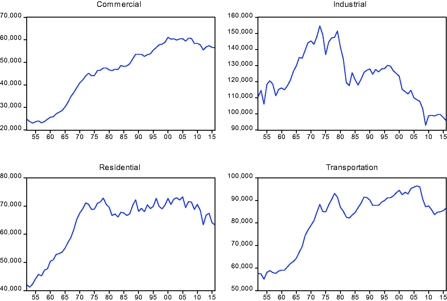
Sectoral energy use in the U.S. during the period 1952–2016.

Figure 2.

The share of each sector in total energy consumption.

The transportation sector makes up approximately 26% of the total U.S. GHG emissions in 2016. At the same time, industrial, residential, and commercial sectors emit about 19%, 14%, and 12% of total GHG in the U.S. The primary reason for the observed differences among the sectors, in terms of their share from the GHG emissions, is the mix of energy sources that each sector relies the most. For example, transportation heavily relies on petroleum, while the commercial and residential sectors mostly use natural gas and electricity. Only a few portion of the energy used in these sectors are from direct consumption of fossil fuels. Therefore, the energy-related emissions from these sectors were low. However, electricity generation itself accounts for 25% of total GHG emission in the U.S. So, emissions from the residential and commercial EN would be much higher when emissions from the electricity generation are included.

We now start the analysis with several widely used unit root tests to examine the presence of a unit root in the data. To that end, we use the ADF,³⁷ DF ^GLS ,⁴⁰ Phillips and Perron,⁴¹ and the ERS³⁹ point optimal unit root tests. To select the lag length, we follow the recursive t-statistic approach of Ng and Perron.⁴⁵ We set $p_{\max} = 8$ , if the last lag is significant at the 10%, we use 8 as the lag length; however, if the last lag is insignificant, we set p = 7 and continue until the last lag becomes significant.^w Ng and Perron⁴⁵ have shown that this approach yields a test statistic that has a better power and size properties compared to the lag lengths determined using Akaike or Schwarz Bayesian information criteria.

The results from the unit root tests without and with a time trend are reported in Table 1. According to the results from the DF ^GLS and ERS tests, all the variables contain a unit root and appear to be non-stationary. The ADF and Phillips–Perron are the only unit root tests that provide some evidence of stationarity; based on the results from these tests, ENR and ENC appear to be stationary at the 5% and 10% significance levels, respectively.^x

Table 1.

Results from the unit root tests.

	With a constant				With a constant and a time trend
	ADF	Phillips–Perron	DF $&^{G L S}$	ERS	ADF	Phillips–Perron	DF $&^{G L S}$	ERS
ENR	−3.12**	−3.29**	−0.58	119.21	−1.10	−1.10	−0.66	78.54
ENC	−2.78*	−1.83	−0.73	133.70	−1.48	−0.32	−1.74	28.49
ENI	−0.70	−0.70	−0.83	11.43	−1.72	−1.65	−1.17	35.83
ENT	−2.05	−1.93	−0.47	58.04	−1.23	−0.82	−1.23	29.18

Note: *and **show rejection of the null of unit root at 5% and 1% level. Lag lengths are selected using t-sig approach.

As an alternative method, we proceed to construct the 90% confidence intervals^y for the sum of the AR(p) coefficients, $α,$ in the usual ADF form. The OLS point estimates of $α$ are reported in column 3 of Table 2. The reported αs ranges from 0.932 to 0.973; however, it is well-known that the OLS point estimates are biased downward and these αs must be used cautiously. In addition, it is well-known that most unit root tests suffer from size distortion and low power when there is a root local-to-unity, as we found in the series.^z To provide more information about the persistence degree of EN, we construct the 90% confidence intervals using the grid-bootstrap approach of Hansen³³ and the equal-tailed and symmetric subsampling approaches of Romano and Wolf.^34, ^aa

Table 2.

The confidences intervals constructed using different approaches.

	Lags	${\hat{α}}_{o l s}$	Grid-bootstrap	Subsampling equal‑tailed	Subsampling symmetric
The 90% confidence intervals
ENR	1	0.932	[0.904, 0.992]	[0.894, 1.005]	[0.864, 0.9996]
ENC	4	0.973	[0.962, 1.002]	[0.967, 1.002]	[0.949, 0.997]
ENI	1	0.971	[0.952, 1.073]	[0.938, 1.018]	[0.876, 1.066]
ENT	2	0.966	[0.947, 1.016]	[0.949, 1.021]	[0.918, 1.014]
The 95% confidence intervals
ENR	1	0.932	[0.896, 1.004]	[0.961, 1.004]	[0.946, 1.0003]
ENC	4	0.973	[0.958, 1.006]	[0.928, 1.110]	[0.837, 1.104]
ENI	1	0.971	[0.929, 1.084]	[0.875, 1.015]	[0.861, 1.003]
ENT	2	0.966	[0.942, 1.020]	[0.943, 1.021]	[0.914, 1.018]

Note: Stationary cases are shown in bold.

Table 3.

Descriptive statistics of the residuals of the models with the selected lags.

	Residential	Commercial	Industrial	Transportation
Mean	0.007	0.002	0.001	0.004
Median	0.011	0.004	0.002	0.007
Maximum	0.057	0.041	0.106	0.068
Minimum	−0.075	−0.049	−0.109	−0.053
Std. Dev.	0.03	0.022	0.041	0.022
Skewness	−0.541	−0.111	−0.436	−0.274
Kurtosis	2.627	2.342	3.62	3.739
Lags	1	4	1	2
Jarque-Bera	3.543	1.305	3.101	2.292
Probability	0.17	0.521	0.212	0.318

The 90% confidence interval for α based on the Hansen’s³³ grid-bootstrap approach using 1999 replications, and a grid with 200 gridpoints^bb are shown in the column 4 in Table 2. The results, which are bias-adjusted, show that the upper bound of the 90% confidence interval is larger than 1 for all series, except for ENR. Therefore, ENC, ENI, and ENT are non-stationary, while ENR appear to be stationary. The lower bound of the calculated confidence intervals range from 0.904 to 0.962, which shows that all the series are highly persistent. So even if we accept that ENR is stationary, it would be highly persistent and shocks would last for a very long period.

The results from the Romano and Wolf’s³⁴ equal-tailed and symmetric subsampling confidence intervals are reported in the columns 5 and 6 in Table 2, respectively. The subsample size or block size was selected based on the algorithm proposed by Romano and Wolf³⁴ with k = 2, b_small = 6, and $b_{b i g} = 19.$ ^cc Based on the equal-tailed subsampling approach, the upper bounds of the confidence intervals of all series are larger than 1; therefore, these time-series have a unit root and are non-stationary. In addition, the lower bounds of the estimated confidence intervals of the sectoral ENs are greater than 0.894, which indicates a very high persistency.

Column 6 in Table 2 shows the estimated confidence interval for the sum of the AR(p) coefficients using the symmetric subsampling approach of Romano and Wolf.³⁴ The results for ENI and ENT are the same as the ones from the equal-tailed subsampling approach; however, for ENR and ENC, the results are different. Based on the symmetric subsampling results, EN in the residential and commercial sectors is stationary because the confidence interval does not contain 1. Nevertheless, it is worth noting that the upper bound for these two series is very close to unity and their lower bounds are also higher than 0.8, which is a sign of high persistency.^dd

To sum up the results, we will use the results from the subsampling symmetric approach of Romano and Wolf³⁴ to determine the persistence degree of the variables. Because, as it mentioned before, the subsampling symmetric approach of Romano and Wolf³⁴ requires fewer assumptions about the nature of e_t, compared with the grid-bootstrapping approach of Hansen.³³ In addition, symmetric confidence intervals have improved coverage accuracies³⁴^,⁴⁶^,⁴⁷ and they are narrower than equal-tailed ones.⁴⁷ Also, they can cope better with some mild misspecifications in residual autocorrelation and have a better performance compared with the subsampling equal-tailed procedure of Romano and Wolf.^34, ^ee Thus, according to the results from the symmetric confidence intervals the EN in the residential and commercial sectors, i.e. ENR and ENC are stationary with a root near to unity. Even though these two variables are stationary, however, their degrees of persistence are different; ENR exhibits the lowest degree of persistence. On the other hand, the estimated confidence intervals show that the ENI and ENT are non-stationary.^ff

The stationarity property of energy use in the building sector (commercial and residential sectors) shows that the energy conservation^gg or demand-management policies in these two sectors would have a transitory effect. But, these policies would be useful to change the EN pattern in the industrial and transportation sectors permanently. Moreover, as the lower bound of the constructed confidence interval in the residential and commercial sectors is very high, so any intervention in the EN in these sectors also would be justified because the effect of the intervention will last for a very long time.

In order to assess the robustness of the results, we also consider the 95% confidence intervals for the sum of the AR(p) coefficients. The results from the 95% confidence intervals are reported in the bottom portion of the Table 2. According to these results, all confidence intervals include 1; therefore, all of the sectoral ENs are non-stationary at the 95% level.^hh

Conclusion

This paper differs from the most of the previous studies at least in two ways. Not only we use different unit root tests to probe the persistence of the energy consumption, but also we construct the 90% confidence intervals for the sum of autoregressive roots in the AR(p) models to examine the stationarity and degree of persistence of energy use in the U.S. during 1952–2016. In addition, instead of studying the aggregate energy use, we examine the energy consumption in the commercial (ENC), residential (ENR), industrial (ENI), and transportation (ENT) sectors in the U.S.

The results from the unit root tests provide some evidence of stationarity for ENR and ENC only. The energy consumptions in the other sectors appear to be non-stationary. On the other hand, constructing the 90% subsampling confidence interval for the sum of an AR(p) coefficients shows that the upper bounds of the confidence intervals for the ENR and ENC are less than $1$ ; therefore, the energy use in these two sectors is stationary but highly persistent.

To sum up the results, we use the results from the 90% symmetric subsampling confidence intervals, because they have a better performance compared to the other methods used in this study. While the ENR and ENC appear to be stationary, the results are in favor of non-stationarity of ENI and ENT. In other words, shocks to the use of energy in the industrial and transportation sectors will have permanent effects and will not decay over time. Since the commercial (industrial) sector is the smallest (largest) consumer of energy in the U.S, so this finding is consistent with the conception that the energy use in small (large) sectors is more likely to be stationary (non-stationary).

The policy implications of these findings are as follows. The industrial and transportation sectors are the best candidates to implement policies such as improved energy efficiency standards, energy conservation, carbon-taxes, investment in renewable technologies, and demand-side management to control GHG emissions through reduction of energy consumption. In other words, the U.S. government can control GHG emissions through creating incentives that can promote the industrial and transportation sectors to diversify the energy mix and also create cleaner technologies.ⁱⁱ Similar policies can be applicable in the residential and commercial sectors (building sector) as well, because even though the effects of shocks will not last forever but as energy consumption in these sectors are very persistent, the effects of these shocks will last for a long period of time. So, policies such as adopting and mandating improved building energy codes, house insulations, programmable thermostats, using advanced cooling and heating systems, efficient appliances, and water heaters are among the incentive-based policies that can be used to affect the energy use in the building sector. Raising social awareness also can be beneficial in this regard. The second implication is that the patterns of energy use in different sectors are heterogeneous, so sector-specific measures and strategies must be adopted. Another implication of the findings is that the past values of the sectoral energy use cannot be used to forecast the energy consumption in the future, as we have found that the series are non-stationary or very persistent.

Different factors might affect the persistence of energy use. Existence of environmental policies, the size of the sector, mix of energy sources, and energy intensity are among the factors that might affect the degree of persistence in the energy consumption. Availability of the technologies and financial costs (including the investments) associated with these technologies are also could be considered as important factors that influence the persistence degree of energy consumption.⁴⁸

A possible extension of this study would be to study the factors that affect the integration property of energy use in different countries or sectors. Moreover, the alternative approaches can be used to examine the degree of persistence of the sectoral energy consumption in the US and compare the results with the findings of this paper to shed more light on the sectoral EN. Energy consumptions at the industry level also can be studied to show the intra-sectoral differences in the energy consumptions.

Footnotes

Declaration of conflicting interests

The authors declared no potential conflicts of interest with respect to the research, authorship, and/or publication of this article.

Funding

The authors received no financial support for the research, authorship, and/or publication of this article.

Notes

Firouz Fallahi is an associate professor in economics at the University of Tabriz, Iran. He holds a PhD in Economics from the University of Ottawa, Canada. He is specialized in Economics of the Environment and Industrial Organization.

References

Environmental Protection Agency. Inventory of U.S. greenhouse gas emissions and sinks: 1990-2015. US: Author, 2017.

Torous

Valkanov

Yan

On predicting stock returns with nearly integrated explanatory variables. J Bus 2004; 44: 937–966.

Chen

Lee

CC.

Is energy consumption per capita broken stationary? New evidence from regional-based panels. Energy Policy 2007; 35: 3526–3540.

Narayan

Smyth

Are shocks to energy consumption permanent or transitory? Evidence from 182 countries. Energy Policy 2007; 35: 333–341.

Hsu

Lee

CC.

Revisited: are shocks to energy consumption permanent or temporary? New evidence from a panel SURADF approach. Energy Econ 2008; 30: 2314–2330.

Lean

Smyth

Long memory in US disaggregated petroleum consumption: evidence from univariate and multivariate LM tests for fractional integration. Energy Policy 2009; 37: 3205–3211.

Warr

Ayres

RU.

Evidence of causality between the quantity and quality of energy consumption and economic growth. Energy 2010; 35: 1688–1693.

Apergis

Payne

JE.

Structural breaks and petroleum consumption in US states: are shocks transitory or permanent?

Energy Policy 2010; 38: 6375–6378.

Apergis

Loomis

Payne

JE.

Are fluctuations in coal consumption transitory or permanent? Evidence from a panel of US states. Appl Energy 2010; 87: 2424–2426.

10.

Apergis

Loomis

Payne

JE.

Are shocks to natural gas consumption temporary or permanent? Evidence from a panel of US states. Energy Policy 2010; 38: 4734–4736.

11.

Gil-Alana

Loomis

Payne

JE.

Does energy consumption by the US electric power sector exhibit long memory behavior?

Energy Policy 2010; 38: 7512–7518.

12.

Fallahi

Causal relationship between energy consumption (EC) and GDP: a Markov-switching (MS) causality. Energy 2011; 36: 4165–4170.

13.

Narayan

Popp

Energy consumption-real GDP nexus revisited: empirical evidence from 93 countries, Econ

Modell 2012; 29: 303–308.

14.

Ozturk

Kaplan

Kalyoncu

The casual relationship between energy consumption nd GDP in Turkey. Energy Environ 2013; 24: 727–734.

15.

Yilanci

Tunali

CB.

Are fluctuations in energy consumption transitory or permanent? Evidence from a Fourier LM unit root test. Renew Sust Energy Rev 2014; 36: 20–25.

16.

Zhuang

Xie

Energy consumption, economic development and environmental improvement in China. Energy Environ 2014; 25: 1345–1357.

17.

Hasanov

Telatar

A re-examination of stationarity of energy consumption: evidence from new unit root tests. Energy Policy 2011; 39: 7726–7738.

18.

Apergis

Tsoumas

Long memory and disaggregated energy consumption: evidence from fossils, coal and electricity retail in the U.S. Energy Econ 2012; 34: 1082–1087.

19.

Barros CP, Gil-Alana LA and Payne JE. U.S. Disaggregated renewable energy consumption: Persistence and long memory behavior. Energy Econ 2013; 40: 425-432.

20.

Lean

Smyth

Conditional convergence in US disaggregated petroleum consumption at the sector level, Discussion paper, Monash University, 2015.

21.

Fallahi

Karimi

Voia

MC.

Persistence in world energy consumption: evidence from subsampling confidence intervals. Energy Econ 2016; 57: 175–183.

22.

Belbute

Pereira

AM.

Does final energy demand in Portugal exhibit long memory? A fractional integration analysis. Port Econ J 2016; 15: 59–77.

23.

Carmona

Congregado

Feria

et al . The energy-growth nexus reconsidered: persistence and causality. Renew Sustain Energy Rev 2017; 71: 342–347.

24.

Fallahi

Stochastic convergence in per capita energy use in world. Energy Econ 2017; 65: 228–239.

25.

Fallahi

Voia

MC.

Convergence and persistence in per capita energy use among OECD countries: revisited using confidence intervals. Energy Econ 2015; 52: 246–253.

26.

Aslan

Kum

The stationary of energy consumption for Turkish disaggregate data by employing linear and nonlinear unit root tests. Energy 2011; 36: 4256–4258.

27.

Ajmi

El Montasser

Nguyen

DK.

Testing the relationships between energy consumption and income in G7 countries with nonlinear causality tests. Econ Modell 2013; 35: 126–133.

28.

Hamdi

Sbia

Shahbaz

The nexus between electricity consumption and economic growth in Bahrain. Econ Modell 2014; 38: 227–237.

29.

Farhani

Chaibi

Rault

CO2 emissions, output, energy consumption, and trade in Tunisia. Econ Modell 2014; 38: 426–434.

30.

Shahbaz

Khraief

Mahalik

et al . Are fluctuations in natural gas consumption per capita transitory? Evidence from time series and panel unit root tests. Energy 2014; 78: 183–195.

31.

Pablo-Romero

Sancez-Braza

Residential energy environmental Kuznets curve in the EU-28. Energy 2017; 125: 44–54.

32.

Mishra

Smyth

Conditional convergence in Australia’s energy consumption at the sector level. Energy Econ 2017; 62: 396–403.

33.

Hansen

BE.

The grid bootstrap and the autoregressive model. Rev Econ Stat 1999; 81: 594–607.

34.

Romano

Wolf

Subsampling intervals in autoregressive models with linear time trend. Econometrica 2001; 69: 1283–1341.

35.

Zhang

Target versus price: improving energy efficiency of industrial enterprises in China. Master’s Thesis, Penn State University, USA.

36.

Kruschke

JK.

Bayesian data analysis. Wiley Interdiscip Rev Cogn Sci 2010; 1: 685–676.

37.

Dickey

Fuller

Distribution of the estimators for autoregressive time series with a unit root. J Am Stat Assoc 1979; 74: 427–431.

38.

Said

Dickey

DA.

Testing for unit roots in autoregressive-moving average models of unknown order. Biometrika 1984; 71: 599–607.

39.

O’Reilly

Whelan

DK.

Has Euro-area inflation persistence changed over time?

Rev Econ Stat 2005; 87: 709–720.

40.

Elliot

Rothenberg

Stock

JH.

Efficient tests for an autoregressive unit root. Econometrica 1996; 64: 813–839.

41.

Phillips

PCB

Perron

Testing for a unit root in time series regression. Biometrika 1988; 75: 335–346.

42.

Andrews

Chen

WK.

Approximately median-unbiased estimation of autoregressive models. J Business Econ Stat 1994; 12: 187–204.

43.

Rapach

Wohar

ME.

The persistence in international real interest rates. Int J Fin Econ 2004; 9: 339–346.

44.

Mikusheva

Uniform inference in autoregressive models. Econometrica 2007; 75: 1411–1452.

45.

Perron

Lag length selection and the construction of unit root tests with good size and power. Econometrica 2001; 69: 1519–1554.

46.

Beran

Prepivoting to reduce level error of confidence sets. Biometrika 1987; 74: 457–468.

47.

Hall

On symmetric bootstrap confidence intervals. J R Stat Soc B 1988; 50: 35–45.

48.

Worrell

Ramesohl

Boyd

Advances in energy forecasting models based on engineering economics. Ann Rev Environ Res 2004; 29: 345–381.

49.

Efron

Tibshirani

RJ.

An introduction to the bootstrap. Monographs on statistics and applied probability. New York: Chapman and Hall, 1993.

50.

Maddala

Kim

I-M.

Unit roots, cointegration, and structural change. Cambridge: Cambridge University Press, 1998.

51.

Smyth

Are fluctuations in energy variables permanent or transitory? A survey of the literature on the integration properties of energy consumption and production. Appl Energy 2013; 104: 371–378.

52.

Mishkin

FS.

In‡ation dynamics. Int Finance 2007; 10: 317–333.

53.

Chinn

Wei

SJ.

A faith-based initiative meets the evidence: does a flexible exchange rate regime really facilitate current account adjustment.

Rev Econ Stat 2013; 95: 168–184.

54.

Beck

Hubrich

Marcellino

On the importance of sectoral and regional shocks for price-setting. J Appl Economet 2016; 31: 1243–1253.

55.

Greene

WH.

Econometric analysis. 8th ed. New York: Pearson, 2018.