



Abstract
This article proposes a hybrid technique for a grid-connected solar–wind hybrid system with electric vehicles. The Mexican Axolotl Optimization and wild horse optimizer are the proposed optimization techniques. The wild horse optimizer improves the axolotl's life behavior. As a result, the proposed scheme is conducted while reducing the annualized cost of the system and utilizing the proposed method. Using modern optimization approaches, the component is sized to achieve the lowest levelized cost of electricity by decreasing the loss of power supply probability. Lastly, the sensitivity analysis is performed to analyze the influence of maximum grid sales and buy capabilities on levelized cost of electricity. The proposed technique's performance is then executed in MATLAB environment and compared to several current methodologies. As a result of the simulation outcomes, the efficiency and performance of the current method are compared to other techniques. According to simulation outcomes, the energy management system (EMS) may lower general expenses by more than 55% and 29% in summer and winter, respectively, while ensuring the satisfaction rate of demand for electric vehicle-charging without knowing the departure times of electric vehicles.
Keywords
Introduction
In current years, electricity scarcity and environmental stress are getting more and more severe, and conventional gasoline motors are inflicting increasing problems because of their excess electricity intake and carbon emissions.1–3 An electric vehicle (EV) is a powerful manner to lessen China's dependence on oil assets and enhance environmental pollution. 4 As a result, the variety of EVs is anticipated to develop exponentially over a couple of years. 5 At present, EV enterprise remains on the level of improvement and one of the vital elements proscribing its improvement is the shortage of charging infrastructure. 6 By November 2019, China has constructed 496,000 public charging piles and 678,000 non-public charging piles, a long way under expectations.7,8 In order to sell the improvement of EV enterprise, the development of speedy EV charging stations (CSs) is essential. 9
Compared with gradual charging, speedy charging has the drawback of big electricity call for and fantastic effect on the country-wide electricity grid 10–15. In order to resolve this problem, wind electricity, photovoltaic (PV) electricity technology, and energy storage structures are carried out in speedy CSs and secure charging providers for EVs.16,17 The utility of wind, PV electricity technology, and energy storage systems (ESS) to speedy EV CSs cannot most effectively lessen fees and environmental pollution, but lessen the result on the software grid and acquire stability of electricity delivery.18,19
It is dangerous for the growth of fast EV CSs with wind, PV electricity, and ESS to anticipate EV weight demand and determine the capability configuration of device components.20–22. A great deal of capabilities will increase the waste of fees and resources. While low capability cannot satisfy the weight need, a large quantity of strength is required from the national energy grid, which can irritate the effect on the software grid. 23 At present, many students have performed research on capability configuration of EV CSs.24–26 According to the present research, the principle elements affecting capability configuration are the weight of the device, the optimization goal, and the optimization method. 27 A hybrid technique for grid-connected solar–wind hybrid system with EVs is proposed in this article. The proposed optimization system is Mexican Axolotl Optimization (MAO) and wild horse optimizer (WHO). The axolotl's life behavior is enhanced by WHO. The rest of the manuscript is organized as below. The sections ‘Introduction’ and ‘Recent research works’ depict the introduction and literature survey, the section ‘Mathematical modeling of electric vehicle CS’ depicts system modeling, and the section ‘Operational strategy and objective function’ depicts reliability process. The section ‘Proposed methodology of electric vehicle CS’ depicts the proposed system. The section ‘Result and discussion’ depicts the simulation result and discussion and lastly, the section ‘Conclusion’ completes the manuscript.
Objectives and contribution
A hybrid technique for the grid-connected solar–wind hybrid system with EVs is presented. The proposed optimization technique is a combination of MAO and WHO. The axolotl's life behavior is enhanced by the WHO. In the MATLAB/Simulink working platform, the performance of the proposed method is evaluated from the existing systems.
The main novelty of the proposed work is to get the overall optimal solution collected from the search space of these operators.
The sizing of the component is executed to get a levelized cost of electricity (LCOE) while reducing the loss of power supply probability (LPSP) with current optimization systems.
The performance of the proposed system is performed at the matrix laboratory/Simulink working platform and the performance is evaluated with existing systems such as artificial bee colony (ABC) and particle swarm optimization (PSO). The energy consumption of the proposed system achieves 720.34 KJ.
Recent research works
Several research works were earlier presented in the literature that depends on EV fast CSs using renewable energy sources with dissimilar systems and features. Here, a part of them is revised.
Li et al. 28 have completed micro-grid energy distribution composed together with wind energy and PV, EVCSs, and ESS. They also considered the uncertainty of EVs’ charging call and dispensed renewable power output. A sturdy optimizing version proposed the region of CSs with dispensed power and primarily based totally on the combined street community and grid. The kernel density estimation approach was utilized to enhance the over-conservatism problem of the study optimization. Lei and Mohammadi 29 have defined a secured power control structure for every islanded along grid-linked operation modes of renewable hybrid AC–DC microgrids thinking about diverse renewable power sources. In the study, the whale optimization algorithm was developed at a finite operational cost of the grid that primarily depends on sequential hypothesis testing technique to determine the identity-primarily based totally cyber-attacks on wireless-primarily based totally advanced measurements infrastructures. Ekren et al.30 have supplied a wind sun hybrid power CS that was designed and optimized via HOMER software. The method of sizing became appropriate everywhere across the world. Deshmukh and Pearce 31 have defined the power-associated factors of growing EV CSs powered with sun PV canopies constructed in the parking infrastructure of large-scale retailers. The car parking zone regions are positioned in the maximum EV marketplace and the technical evaluation was completed with price station prices and capacity of the pinnacle 10 EV.
Guo et al. 32 have elucidated at the top of the line danger evaluation of microgrid integrated using an electric-powered automobile parking lot, call for a reaction program (as rising bendy resources), and unnecessary penetration of renewable strength (wind and sun energies) to beautify the economic as well as environmental goals. To suggest the models using the device operator for every day scheduling with PV along wind energy variation, real-time energy market, load variation, and electrical automobile drivers conduct, conditional value-at-danger for the danger degree criterion became exploited. Emrani-Rahaghi and Hashemi-Dezaki 33 have supplied to fill the sort of studies hole using introducing the probabilistic scenario-primarily based on renewable strength sources’ and strength price's uncertainty. The scenario-primarily based totally version for optimizing REH operation value became tested using the contrast of take a look at effects and Monte Carlo simulation (MCS)-primarily based totally ones.
Ahrabiet al. 34 have executed a hybrid information gap decision theory (IGDT)-stochastic approach to clear up a transmission-restricted AC unit dedication version included using electric powered automobile (EV), incentive-primarily based totally demand response program (DRP), as well as wind strength. The uncertainty behavioral associated with EV proprietors became modeled by the use of a scenario-primarily based totally approach. Additionally, an IGDT approach became implemented to control wind strength uncertainty beneath the degree optimization version.
Shakti Singh et al. 35 have performed grid-connected solar–wind hybrid system to supply electric load request of less shopping complex positioned at the university campus in India. Ephraim Agyekum et al. 36 have illustrated hybrid power plant potential in northern Ghana for the generation of electricity, environmental impact, farmland irrigation, and employment potential. Ampah et al. 37 have used Ghana as a case study to explain six distinct 100% HRES depends on power plants of solar, wind, and biomass for covering the energy requirements of 70 and 30 battery EVs, correspondingly. Praveenkumar et al. 38 have elucidated techno-economics and environmental impact of solar PV (SPV) power plant for electricity and hydrogen production at five dissimilar positions in India (i.e., Chennai, Indore, Kolkata, Ludhiana, and Mumbai). He and Fathabadi 39 have provided a novel standalone CS fed by solar energy and supporting fuel cell stack has been constructed to charge EVs. Bilal et al. 40 have illustrated several hybrid energy system configurations to see the power requirements of EVCS located at the northwest area of Delhi, India.
Background for the research work
The research works suggest that EV speedy CSs with renewable electricity reasserts were the maximum hard task. Moreover, the uncertainty of electricity hubs has attained a super attention deal. Residential electricity hubs were adversely impacted due to device uncertainty including uncertain output strength of renewable distributing units and stochastic behaviors of electrical automobiles owners. The output strength of renewable-primarily fed totally dispensed generations (DGs) and strength price lists in the operation of residential electricity hubs. However, the MCS-primarily based totally fashions were thoroughly unique for assessing the operation price of residential electricity hubs thinking in terms of device uncertainty and possibly time-consuming. Other reviewed studies works have taken into consideration the uncertainties of renewable-primarily based totally DGs and strength marketplace rate in most excellent electricity hubs operation concurrently. Also, the present works on the subject of residential electricity hubs making plans did now no longer concurrently remember uncertainties of renewable-primarily based totally DGs and strength price lists. Hence, a most excellent answer is needed to remedy an issue. These drawbacks are stimulated to do that studies work.
Mathematical modeling of EV CS
Figure 1 illustrated the schematic diagram of proposed grid-related sun wind hybrid machine, which is a hybrid AC/DC machine. In Figure 1, PCC stands for the point of common coupling. The DC bus is connected to wind turbines (WTs), SPV panels, and a CS, while the electric load is connected up to AC bus. The electricity control is greater important on hybrid AC/DC machine in comparison to a single AC or DC machine. Therefore, a microgrid controller is also proposed to reveal a clean electricity waft among numerous additives of the machine. The certain mathematical fashions of every aspect in the machine are mentioned subsequently.

Overview of electric vehicle charging station.
Wind turbine
The power produced by WT is based on the area through which wind passes and the velocity of wind. The power obtained as WT is calculated as below:

Wind speed at different hours of the year is represented in the form of a curve called probability density function (PDF). If a curve is plotted by considering the variable wind speeds, the area under the curve amid any two wind speeds is equivalent to the probability of the wind amid two speeds. It can be expressed as:




The total power generated PWT (t) from WT is calculated as:

SPV panel
An SPV panel is utilized to harness solar energy and create power. The SPV panels are converted into electricity, while the rest is transformed into heat. Therefore, the solar radiation effect along with temperature on output power is considered. The output of an individual SPV panel is given as:

The cell temperature and variation of power with respect to the changes in temperature are given by:


Electric vehicle charging station
The CS comprised a double converter, charging bays, and EVs. EVs can be charged according to their state of charge (SOC) when a battery is completely charged; it is defined as the available capacity ratio to its maximal capacity. Thus, it defines the remaining charge percentage of the battery.
Mathematically, the practical constraints imposed on the charging of EVs are described as:



Power converter
PV panels and WTs feed DC power to EVs at the CS. However, converters are required to satisfy load demand or supply power to the grid or vice versa. According to the maximum grid sales


Operational strategy and objective function
Figure 1 displays to ensure that the solar–wind hybrid system satisfies the load power demand, where NPV and NWT must be determined. The objective function is created by seeing the reliability and LCOE.
Reliability
A system is considered reliable if it has the adequate power to satisfy the load demand, which depends on LPSP. Two types of load demands are required to be satisfied: the first is the load demand of EVs Pdev (T) and the second is the AC load demand Pac (T). Pdev (T) at T time interval is calculated as: (1) If (2) If (3) If (4) If





When


LPSP can be continued within the exact tolerance band for solving optimal sizing issue. In this study, it is considered that the maximal limit of LPSP is 1%.
Levelized cost of electricity
The main objective of this study is to achieve power exchange between various components of the system and minimize LCOE of the overall proposed system. NPV and NWT required maintaining minimum LPSP and annualized cost of system (ACS). The ACS includes the costs of installing SPV panels and a WT, energy costs purchased and shifted back with grid, and the converter costs.



Annual capital cost
This includes the installation and purchase costs of the components. The capital recovery factor (CRF), annual capital cost of SPV panels, and WTs are calculated as:



Annual replacement cost
The total annual cost of replacing SPV panels and WT is calculated as:


Maintenance cost
It establishes labor, cleaning, and repairing cost in case of temporary damage. The maintenance costs of SPV panels and WTs are calculated as:


Salvage value
The salvage value of a WT and SPV panel is estimated as follows:


Cost of exchanging power
The total quantity of electricity purchased by




Moreover, the cost potency of a system can be determined by the objective function LCOE that is the average COE obtained from the system.





Proposed methodology of EVCS
A hybrid technique for a grid-connected solar–wind hybrid system with EVs is described. The proposed optimization system is a combination of MAO and WHO. MAO algorithm is stimulated by the axolotl's birth, breeding, and restoration of tissues, as they live in an aquatic environment. 41 WHO is stimulated by the environmental behavior of wild horses, exhibiting several behaviors, like grazing, chasing, dominating, leading, and mating. 42 The axolotl's life behavior will be enhanced by the WHO.
Step 1: Initialization and random generation. The initial population of axolotls is generated at random. Then, because axolotls develop differently depending on their sex, every individual is allocated as male or female, yielding two subpopulations.
Step 2: Fitness function. The main objective is minimizing ACS. The component sizing will be done for attaining LCOE when minimizing LPSP

Step 4: Injury and restoration. Axolotls can become injured when traveling across the water. This procedure is taken into account during the injury and restoration phase. If a probability of damage (dp) is met for every axolotl Si on population (male or female), the axolotls will lose a certain part of their body. It loses the jth body part (bit) and interchanges with pji0 mini + (maxi − mini) *ri,. Figure 2 depicts the creation of horse groups based on original population.

Formation of horse groups adapted with initial population.
Step 5: Reproduction and assortment. The male deposits spermatophores, which collect with the female's cloaca and deposit in her sperm. Eggs are formed by the continuous combining of genetic information from both parents (Figure 4). Let us consider that every male and female axolotl takes two eggs. The assortment process begins as the eggs hatch. The freshly formed individuals (larval state) will compete for survival through their parents. If the young outperform them in terms of the objective function, the young will take their place.

Availability of solar photovoltaic (PV) irradiance.
Updation
Updating the male and female population and number of evaluation using WHO.
Step 6:Grazing behavior. In the earlier segment, foals spent the majority of their time grazing everywhere in the institution. To recall, the stallion is the grazing area center, and the institution individuals are looking for the center (graze) for the place to effect grazing behavior.
Step 7:Horse mating behavior. The precise behavior of horses in comparison to other animals and isolating the foals from the institution and mating them. Before reaching adolescence, male foals combine institution of unmarried horses and female foals combine certain own circle of relatives institution.
Step 8:Group leadership. Its leader should guide the institution to a suitable location. We recall the water hole as a suitable location. The institution should be directed toward this water hole. Other enterprises circulate on same direction as this water hole. Leaders compete the water hollow for dominating institution to use this water hollow, until the dominating institution. Figure 3 depicts the Wild Horse Optimization flowchart.

Flowchart of wild horse optimization.
Step 9: Interchange and selection of leaders. First, they chose the leaders at random while keeping the algorithm's nature in mind. In final stages of the algorithm, executives are assured that the primary focus is entirely on health. If the institution participants are in better health than the other, the associated member will shift the site.
Result and discussion
This study proposes a hybrid technique for a grid-connected solar–wind hybrid system with EVs. The proposed optimization system is a combination of MAO and WHO. The axolotl's life behavior will be enhanced by WHO. Therefore, it is the proposed system while minimizing ACS is performed using the proposed algorithms. While minimizing LPSP, component sizing is performed using recent optimization techniques to obtain LCOE. Figure 4 depicts the availability of solar PV irradiance. Here, the irradiance of PV flows 0–0.8 W/m2 at 0 h and 2000 h of time duration the irradiance of PV increased till 1 W/m2. Figure 5 depicts the availability of wind speed. Here, the wind speed flows as of 1–6 m/s at 0 h of time period and it maximized till 20 m/s at 8000 h of time period. Figure 6 depicts the availability of wind speed frequency. Here, the availability of wind speed frequency flows from 0% to 1% at the speed of 1m/s and then at the speed of 5 m/s the wind frequency increased up to 14%. Figure 7 depicts the load demand profile of winter weekday, winter weekend, and summer weekday. Subplot (a) presents the load demand profile of winter weekday. It flows as of 3–5.5 kW at 20 h of time duration and then it reduced till 3 kW at 24 h of time duration. Subplot (b) presents the load demand for winter weekend. It flows 2.5 at 1 h of time period and it remains constant up to 6 h and then it increased from 3.5 to 6.5 kW at 20 h of time duration. Subplot (c) presents the load demand profile of summer weekday. It flows 4 to 3 kW at 2 h of time duration and then it rise still 8.5 kW at 19 h and it declines till 5 kW. Figure 8 depicts the variation in electrical load demand. Here, the electrical load demand flows as of 2–6 kW at 0 h of time period. Figure 9 depicts ASC comparison of MAOWHO and existing system. The MAOWHO and existing PSO and ABC methods are presented. Figure 10 depicts the availability of ACS per year. Here the availability of ASC flows from 2 to 11 at the iteration of 10–100. Figure 11 depicts the monthly power generation and consumption for AC load. Here, the power flows as of 0 to −2.5 MW. Figure 12 depicts the monthly power generation and consumption for EV demand. Here the power flows from 0 to −1.5 MW. Figure 13 depicts the monthly power generation and consumption for grid purchase. Here, the power flows from 0 to 3MW at 1 month and it highly increased as of 0–6.5 at the month of 4. Figure 14 depicts the monthly power generation and consumption for PV power. Here, the power flows from 0 to 3 MV at 1 month and it highly increased up to 10 MV in the month of 9. Figure 15 depicts the monthly power generation and consumption for wind power. Here, the power flows from 0 to 1.5 MV at 1 month and it highly increased up to 5 MV at the month of 9. Figure 16 depicts the monthly power generation and consumption for grid sale. Here, the power flows from 0 to 0.5 MV at 1 month and it highly increased up to 5 MV at the month of 4. Figure 17 depicts the monthly power generation and consumption for excess power. Here, the power flows from 0 to 0.2 MV at 1 month and it highly increased up to 0.23 MV at the month of 6.
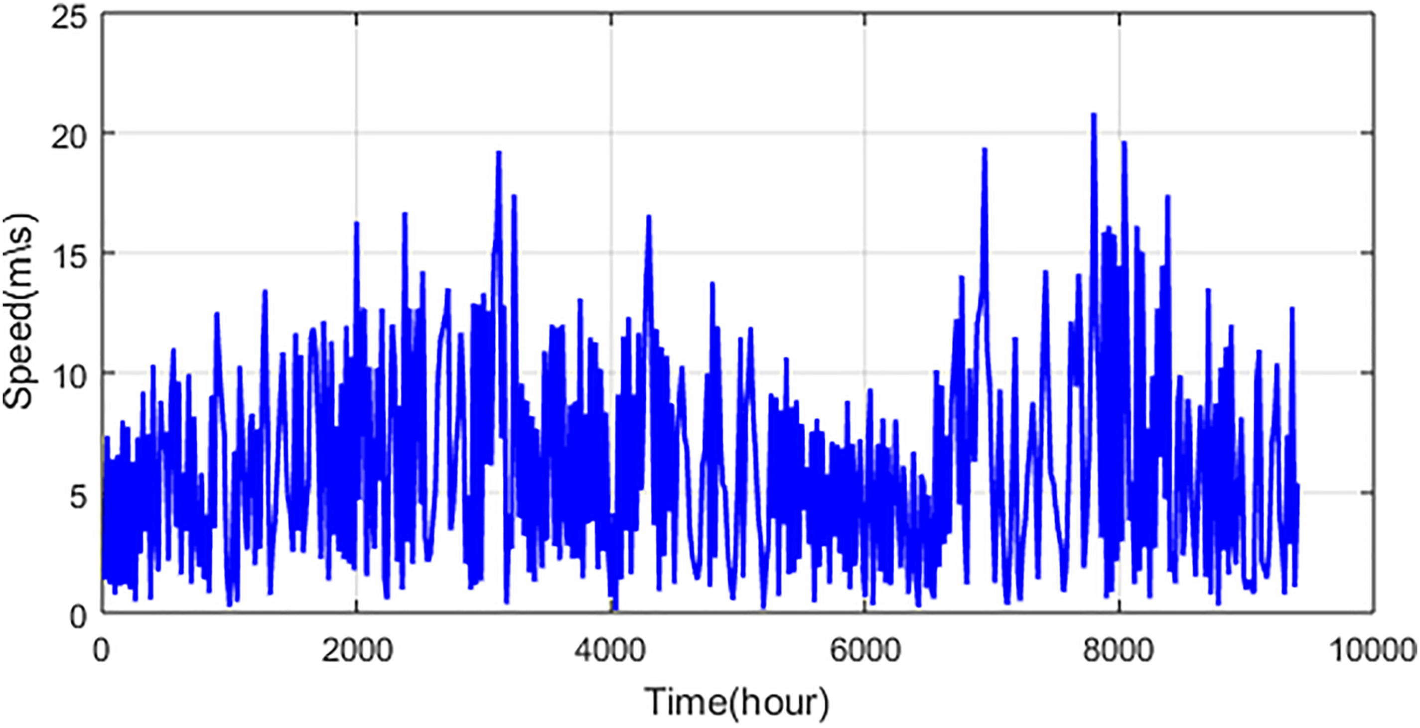
Availability of wind speed.

Availability of wind speed frequency.
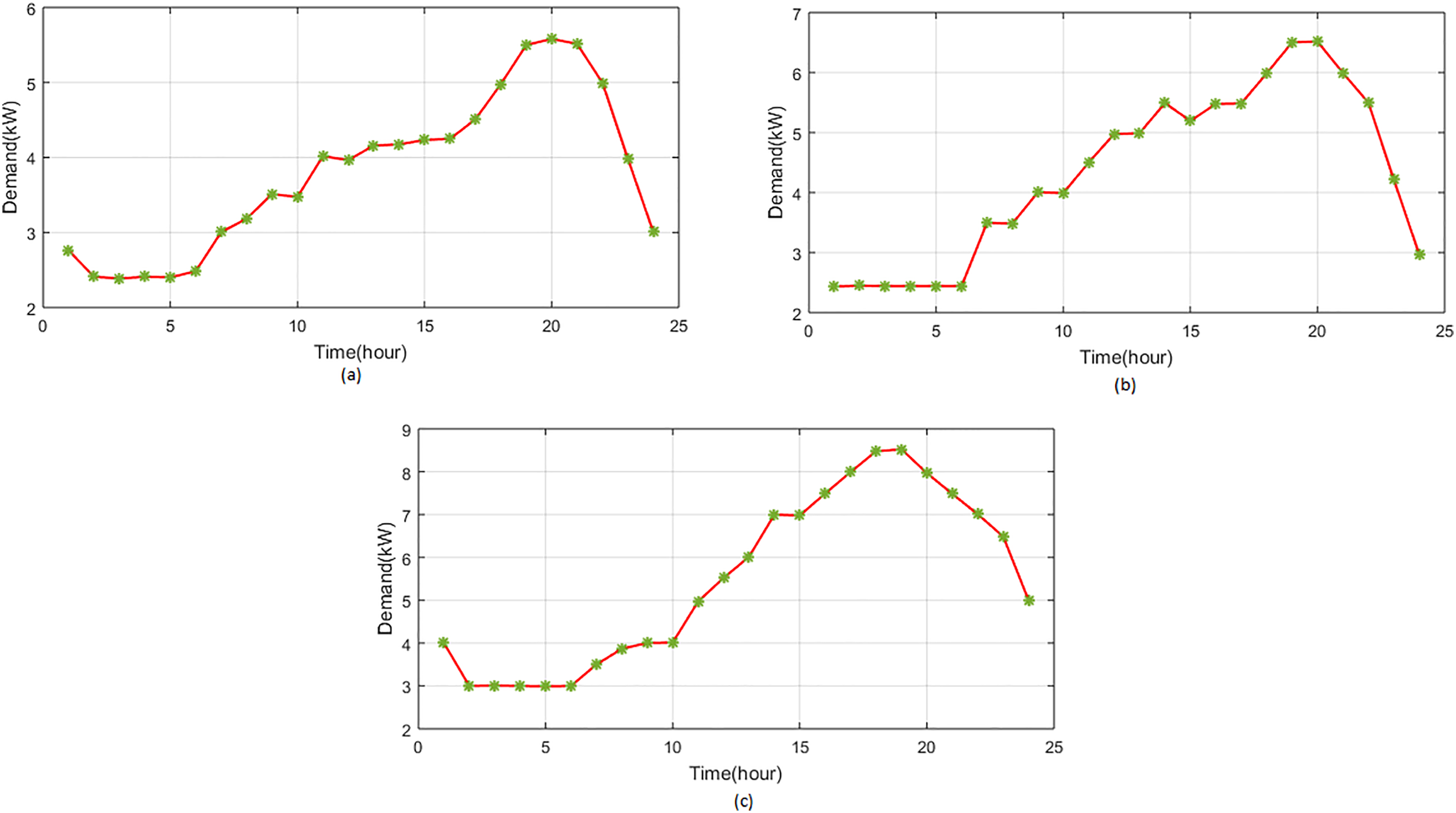
Load demand profile of (a) winter weekday, (b) winter weekend, and (c) summer weekday.

Variation of electrical load demand.

ASC comparison of Mexican Axolotl Optimization and wild horse optimizer (MAOWHO) and existing method.

Availability of ASC per year.
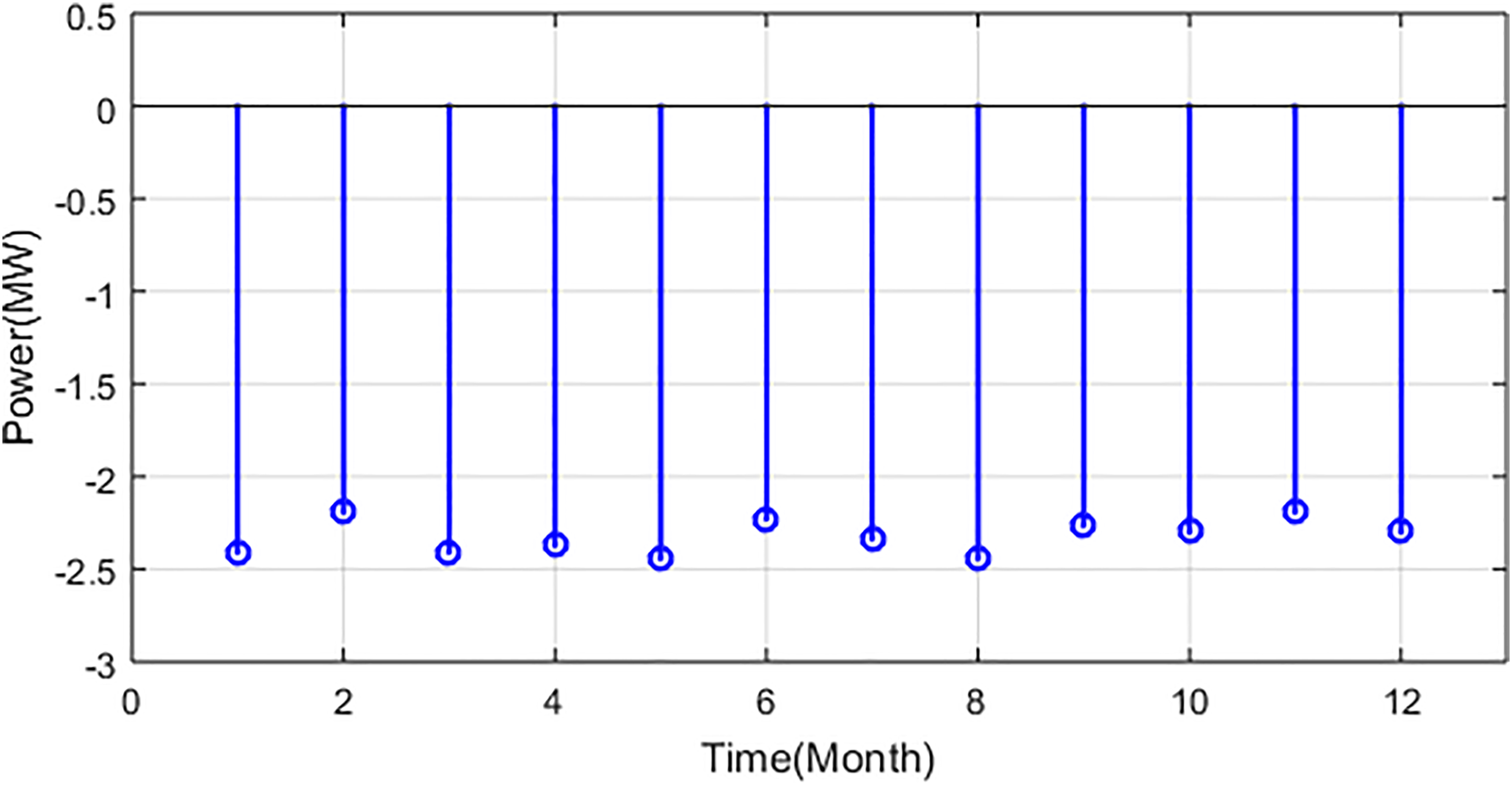
Monthly power generation and consumption for AC load.
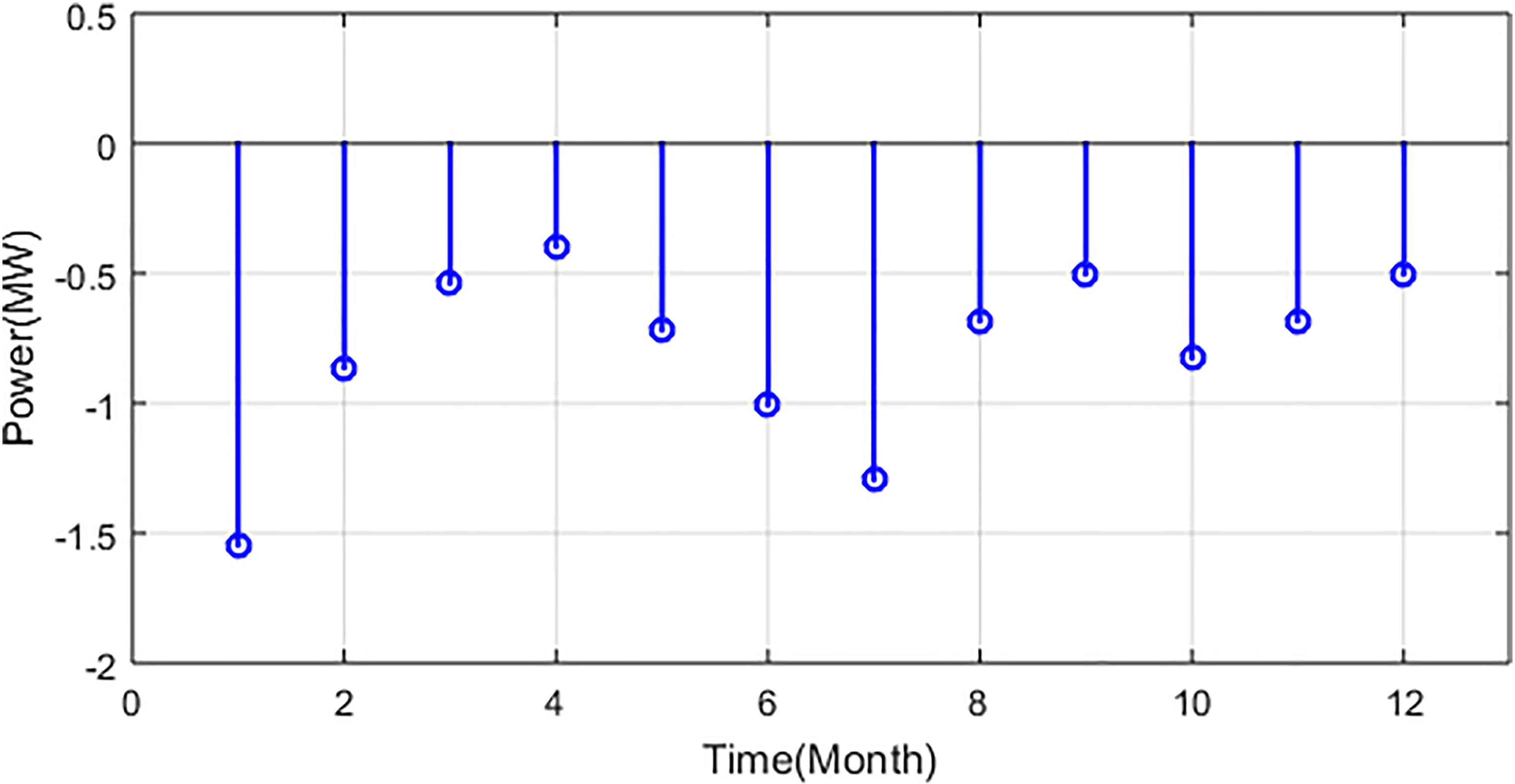
Monthly power generation and consumption for electric vehicle (EV) demand.
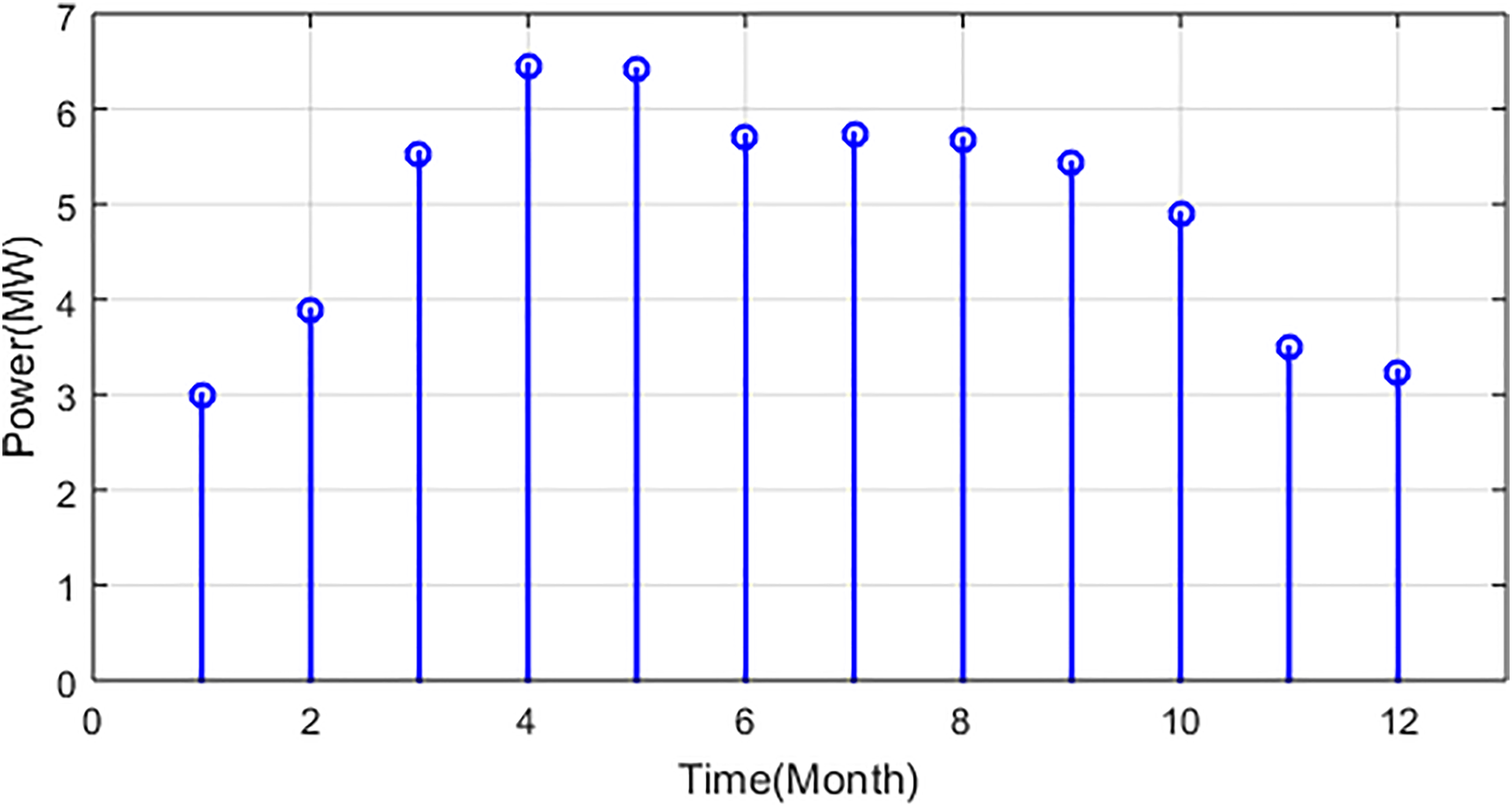
Monthly power generation and consumption for Grid purchase.

Monthly power generation and consumption for photovoltaic (PV) power.
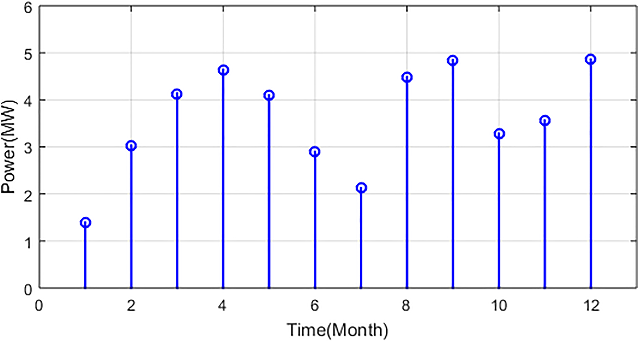
Monthly power generation and consumption for wind power.

Monthly power generation and consumption for grid sale.
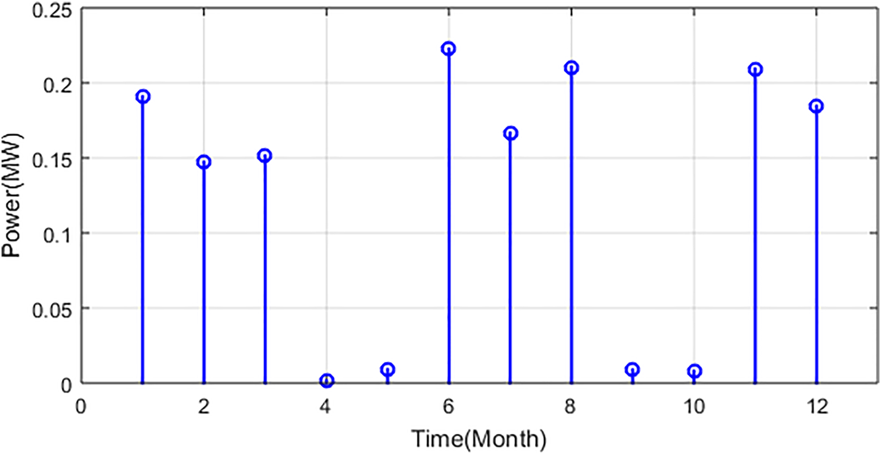
Monthly power generation and consumption for excess power.
Figure 18 depicts the monthly power generation and consumption for unmet load. Here, the power flows from 0 to −3 MV at 1 month and it highly decreased up to −4 MV at the month of 6. Figure 19 depicts the one-day power balance of winter for AC load. Here, the power flows from 0 to −3 MV at 1 h and highly decreased up to −5 MV at 19 h. Figure 20 depicts the one-day power balance of winter for EV demand. Here, the power flows 0 to −9 MV at 9 h and it highly decreased till −20 MV at 12 h. Figure 21 depicts the one-day power balance of winter for grid purchase. Here, the power flows from 0 to −3 MV at 1 h and it highly decreased up to −9 MV at 11 h. Figure 22 depicts the one-day power balance of winter for PV power. It flows from 0 to 6 MV at 10 h and it highly increases up to 29 MV at 14 h. Figure 23 depicts the one-day power balance of winter for wind power. It flows 0 to 3 MV at 9 h and it highly increases up to 13 MV at 15 h. Figure 24 depicts the one-day power balance of winter for grid sale. It flows from 0 to 3 MV at 9 h and it highly increases up to 13 MV at 15 h. Figure 25 depicts the one-day power balance of winter for excess power. It flows from 0 to 3 MV at 9 h and it highly increases up to 13 MV at 15 h. Figure 26 depicts the one-day power balance of winter for unmet load. Here, the power remains constant at 0 till the end. Figure 27 depicts the one-day power balance of summer for AC load. Here, the power flows as of −5 MV and it decreased down to −3 MV. Figure 28 depicts the one-day power balance of summer for EV demand. Figure 29 depicts the one-day power balance of summer for grid purchase. Here, the power flows as of 0–27 MV. Figure 30 depicts the one-day power balance of summer for PV power. Figure 31 depicts the one-day power balance of summer for wind power. Figure 32 depicts the one-day power balance of summer for grid sale. Figure 33 depicts the one-day power balance of summer for excess power. Figure 34 depicts the variation of levelized cost of energy with maximum grid sales and purchase capacities are presented. Figure 35 depicts the one-day power balance of winter for AC load. It flows from 0 to −5 MV at 1 h of time duration. Figure 36 depicts the one-day power balance of winter for EV demand. It flows from 0 to −1 MV at 1 h of time duration. Figure 37 depicts the one-day power balance of winter for grid purchase. It flows from 0 to −5 MV at 1 h of time duration. Figure 38 depicts the one-day power balance of winter for PV power. Figure 39 depicts the one-day power balance of winter for wind power. Figure 40 depicts the one-day power balance of winter for grid sale. Figure 41 depicts the one-day power balance of winter for excess power. Figure 42 depicts the one-day power balance of winter for unmet load. Figure 43 depicts the one-day power balance of summer for grid purchase. Figure 44 depicts the one-day power balance of summer for PV power. Figure 45 depicts the one-day power balance of summer for wind power. Figure 46 depicts the one-day power balance of summer for grid sale. Figure 47 depicts the one-day power balance of summer for excess power. Figure 48 depicts the one-day power balance of summer for unmet load.
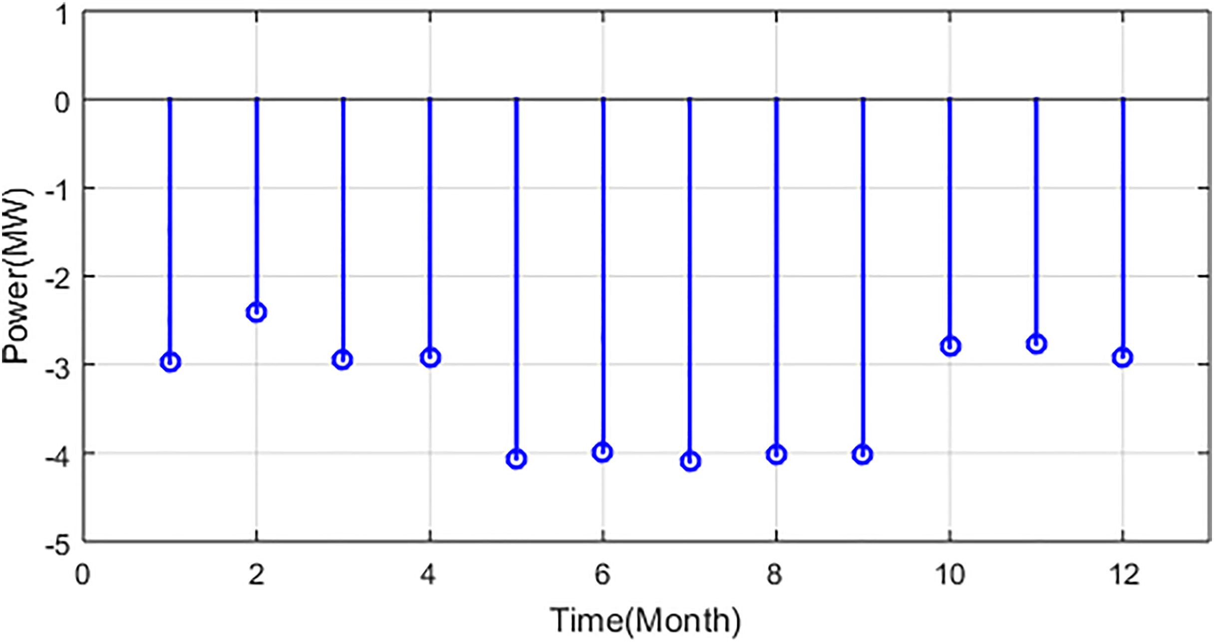
Monthly power generation and consumption for unmet load.
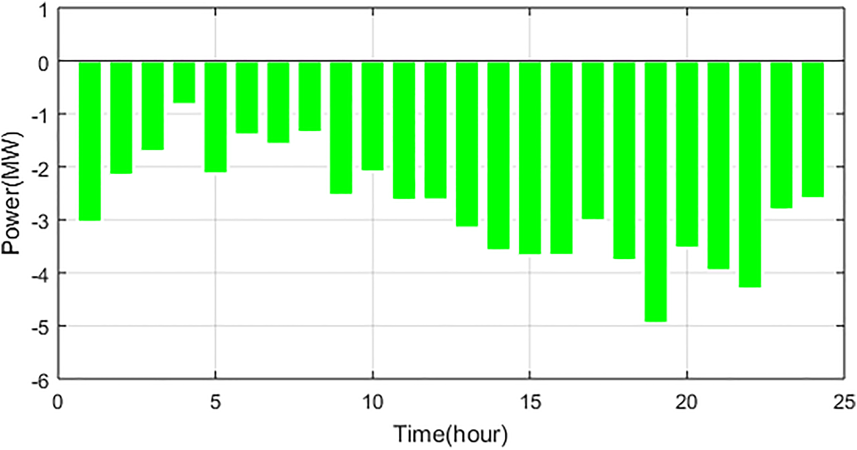
One day power balance of winter for AC load.
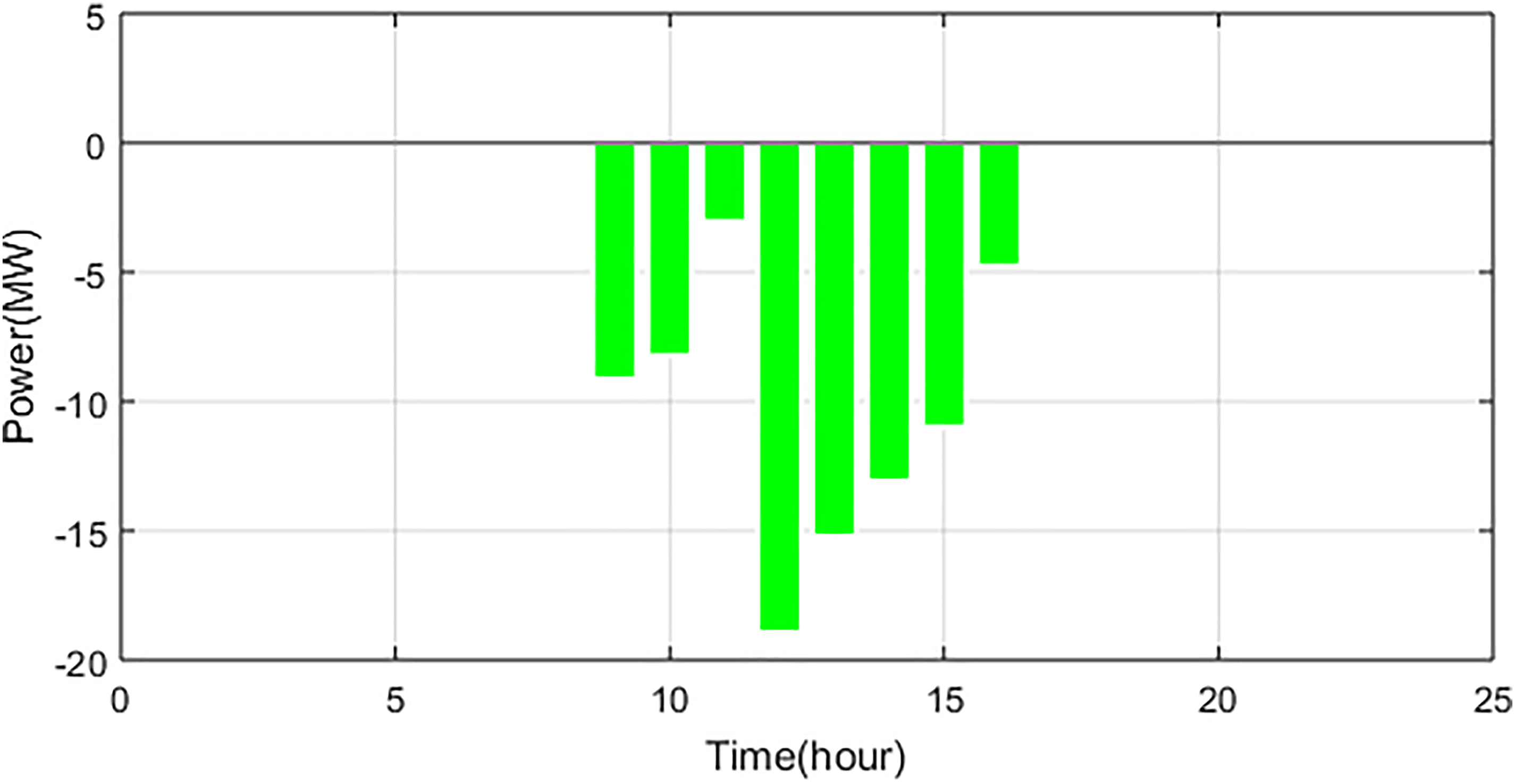
One day power balance of winter for electric vehicle (EV) demand.
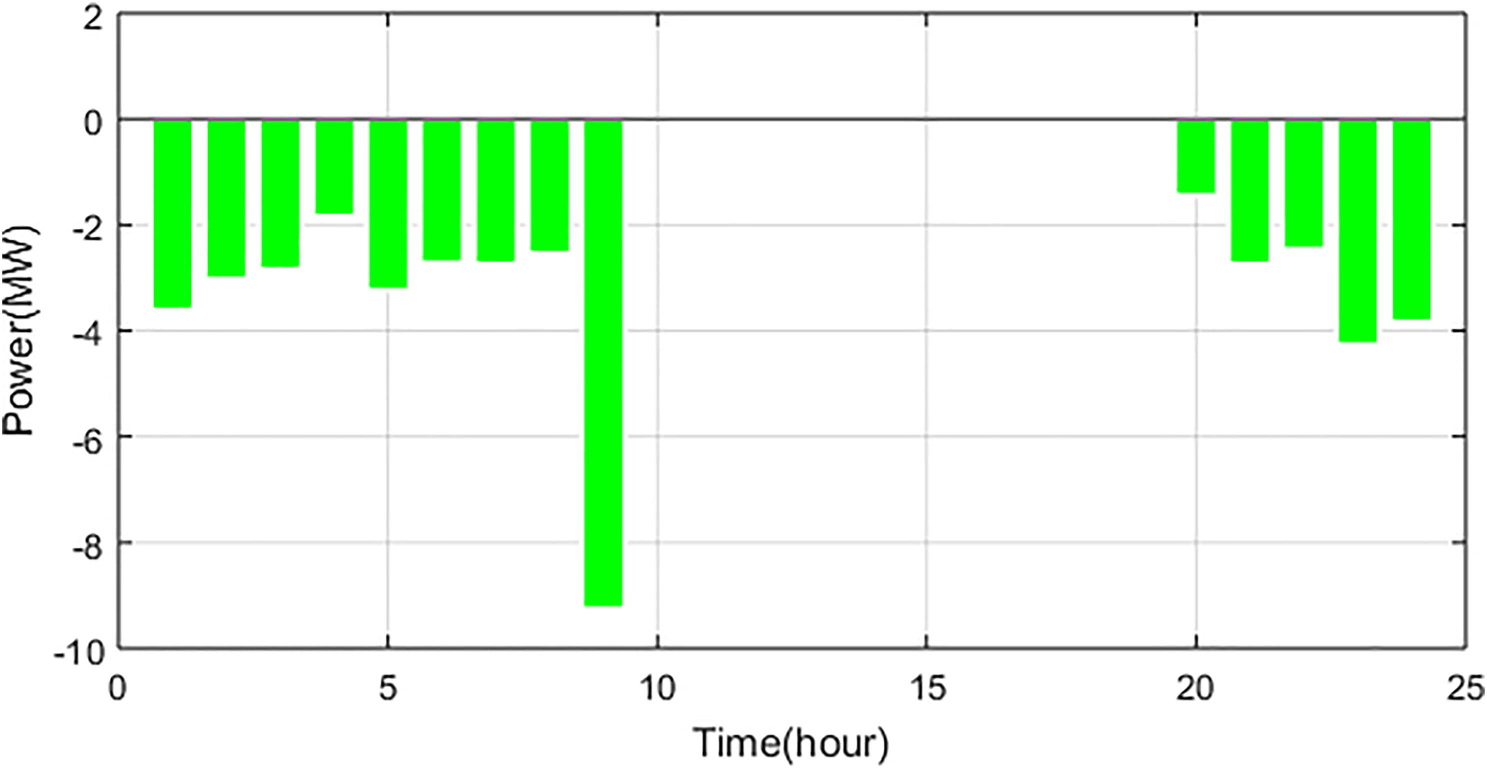
One day power balance of winter for Grid purchase.
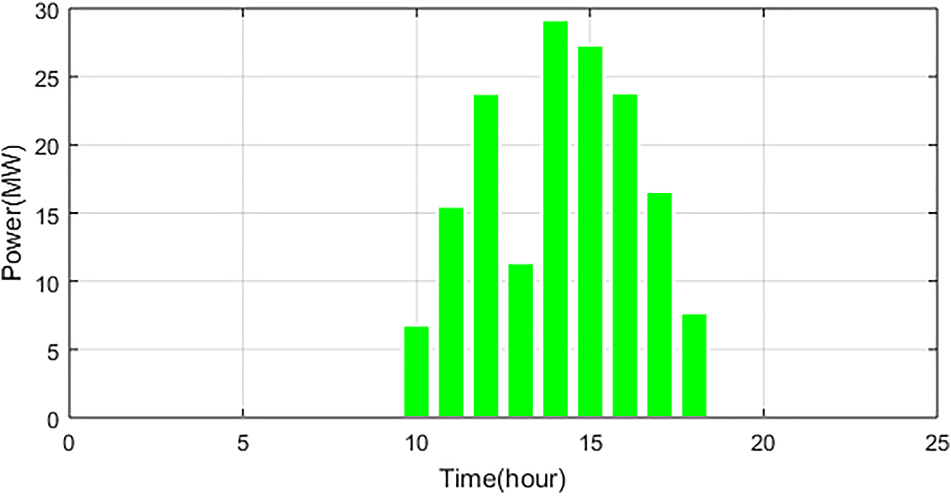
One day power balance of winter for photovoltaic (PV) power.

One day power balance of winter for wind power.
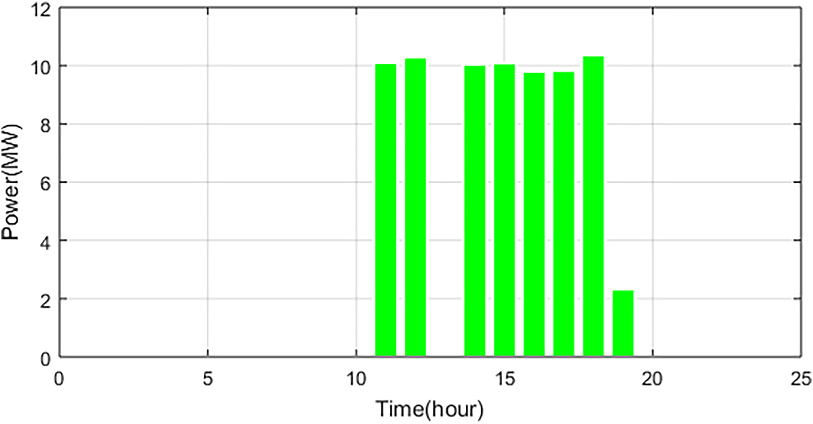
One day power balance of winter for grid sale.

One day power balance of winter for excess power.

One day power balance of winter for unmet load.
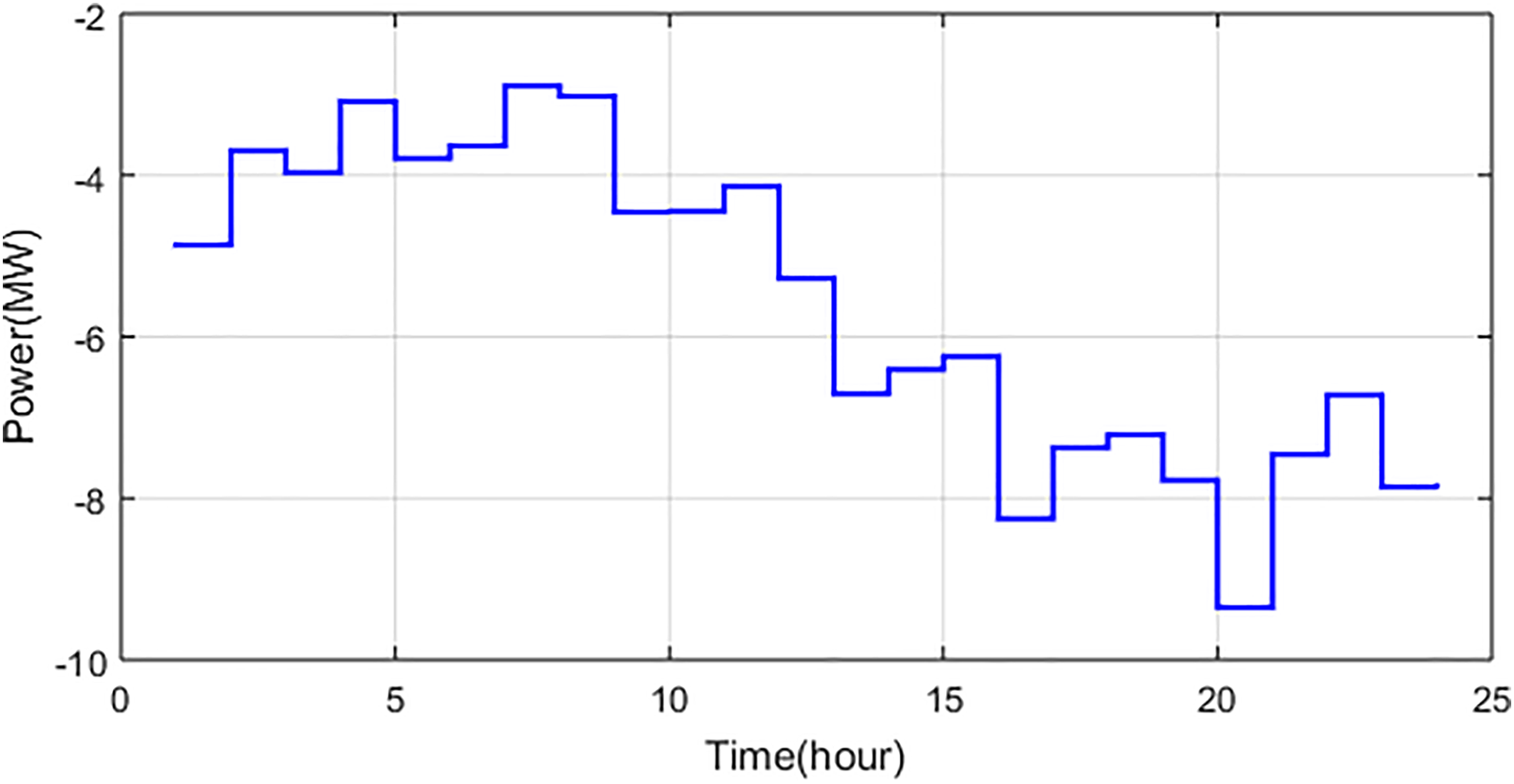
One-day power balance of summer for AC load.
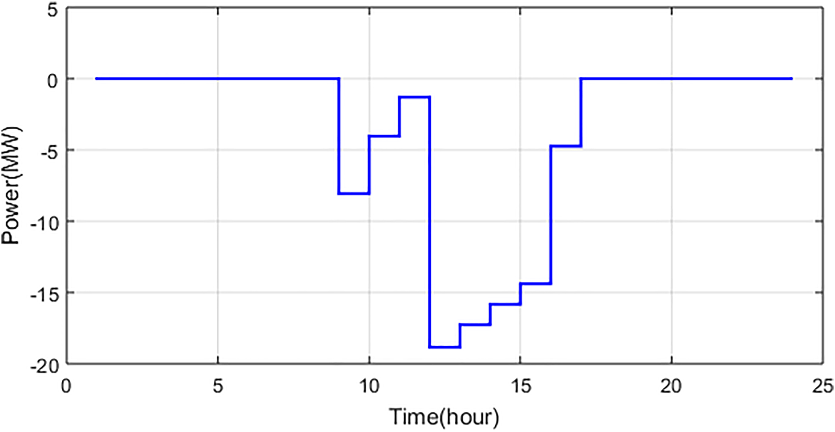
One-day power balance of summer for electric vehicle (EV) demand.

One-day power balance of summer for grid purchase.

One-day power balance of summer for photovoltaic (PV) power.

One-day power balance of summer for wind power.
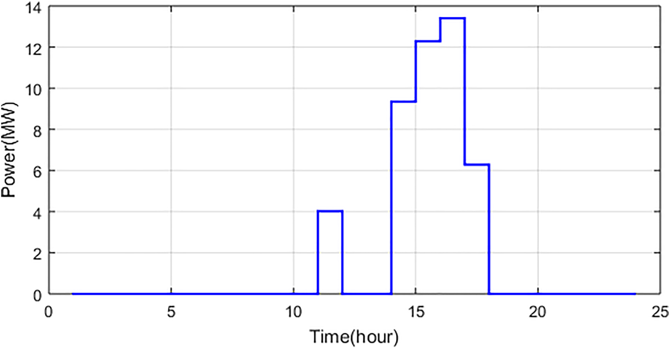
One-day power balance of summer for grid sale.

One-day power balance of summer for excess power.

Variation of levelized cost of energy with maximum grid sales and purchase capacities.
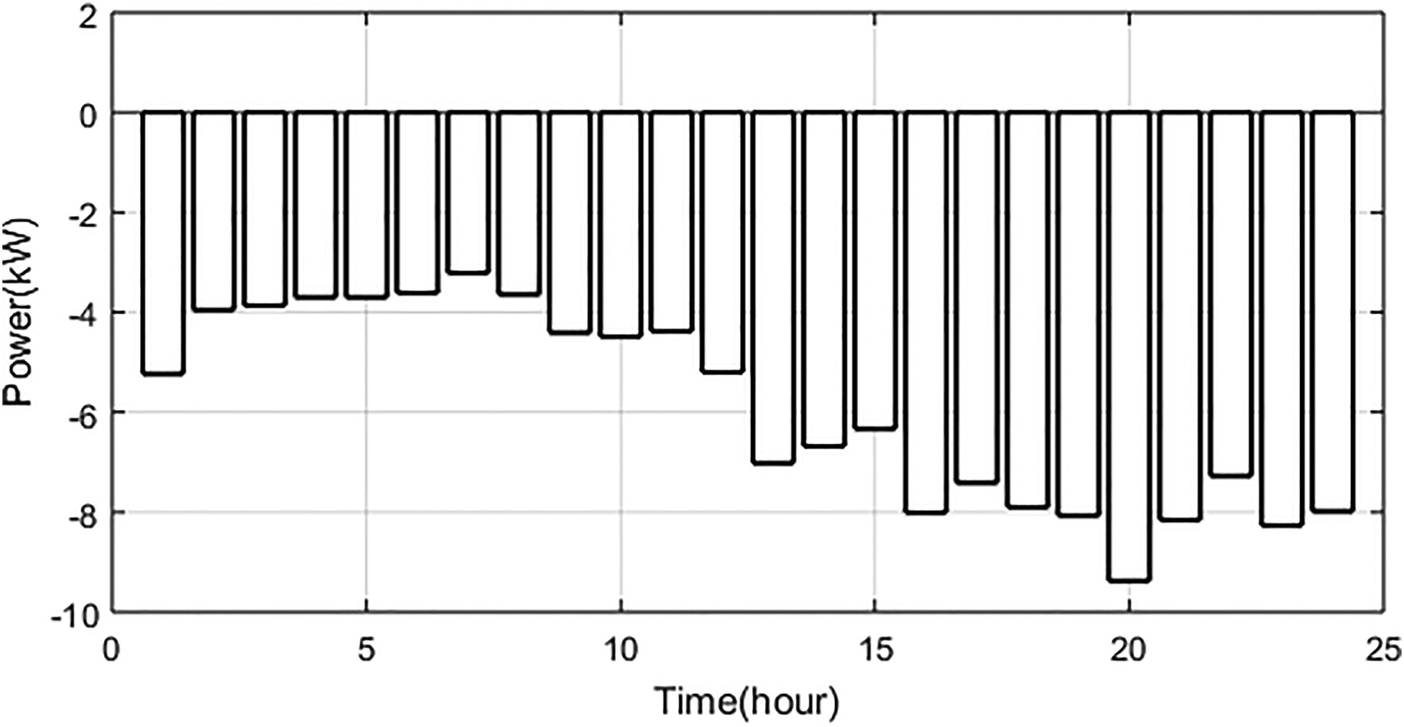
One-day power balance of winter for AC load.
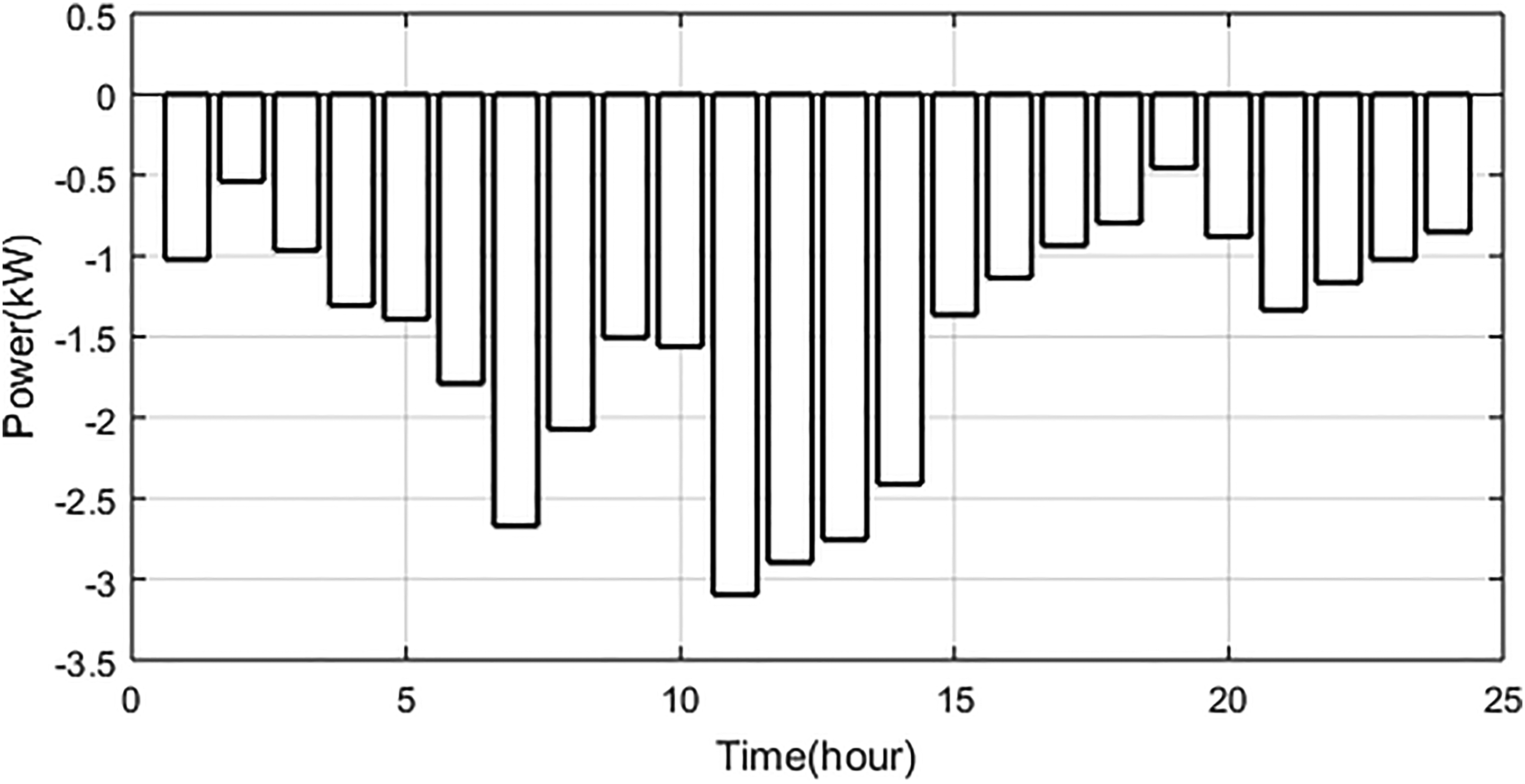
One-day power balance of winter for electric vehicle (EV) demand.

One-day power balance of winter for grid purchase.

One-day power balance of winter for photovoltaic (PV) power.
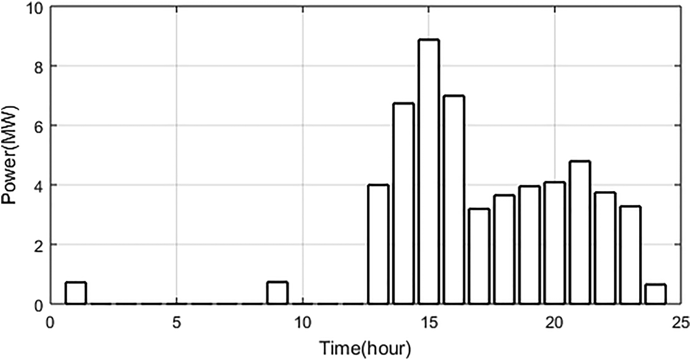
One-day power balance of winter for wind power.
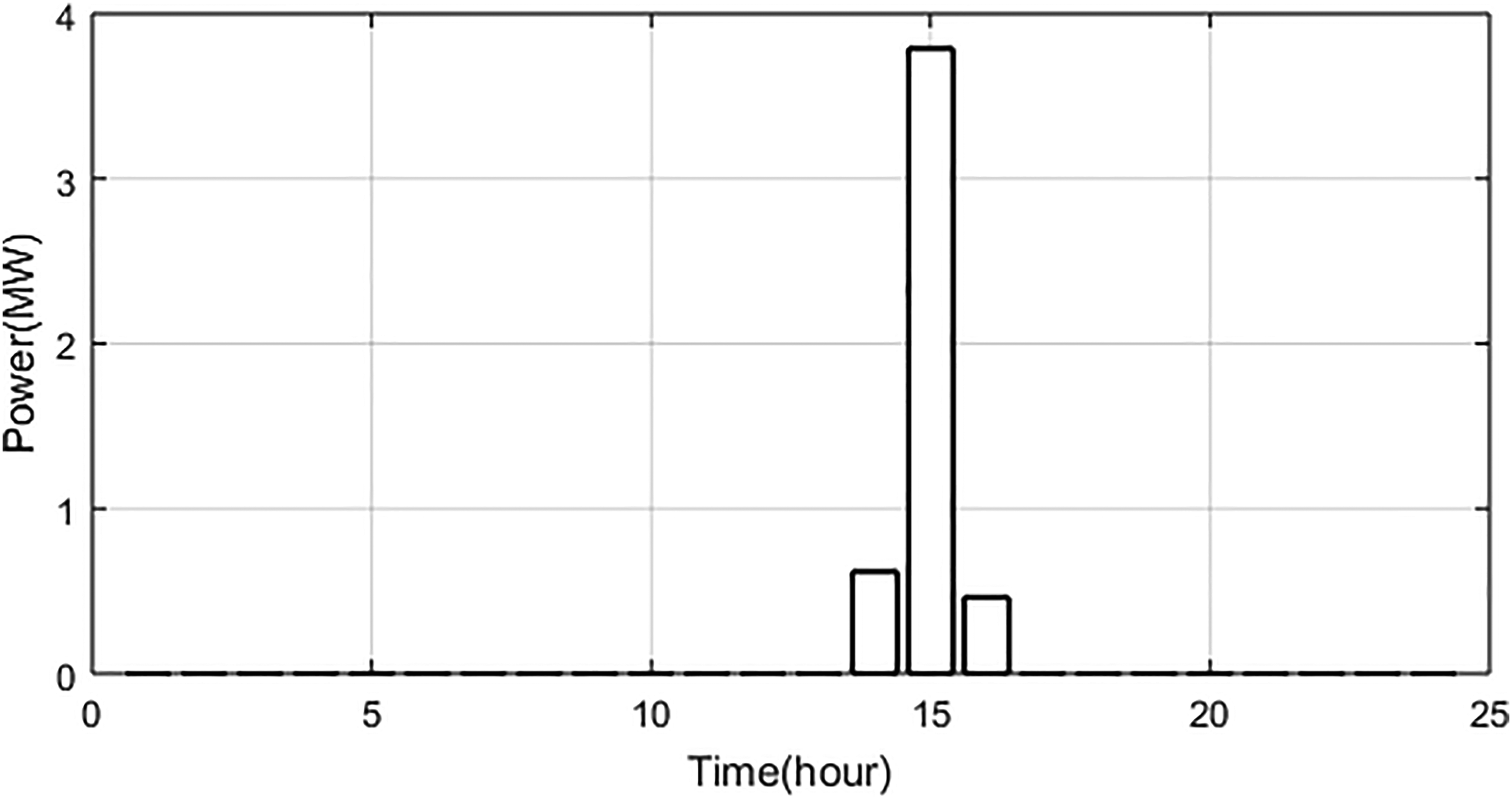
One-day power balance of winter for grid sale.

One-day power balance of winter for excess power.
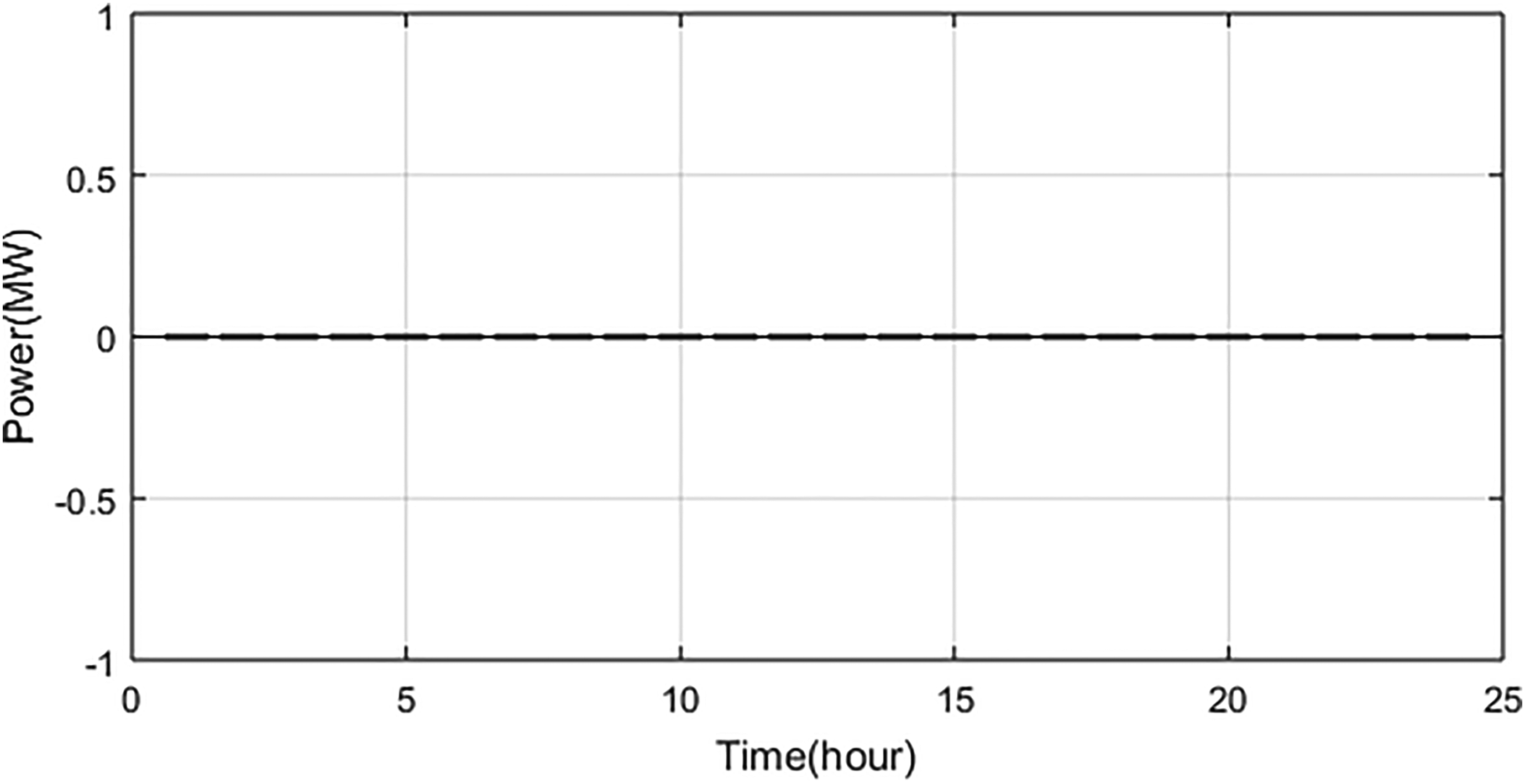
One-day power balance of winter for unmet load.
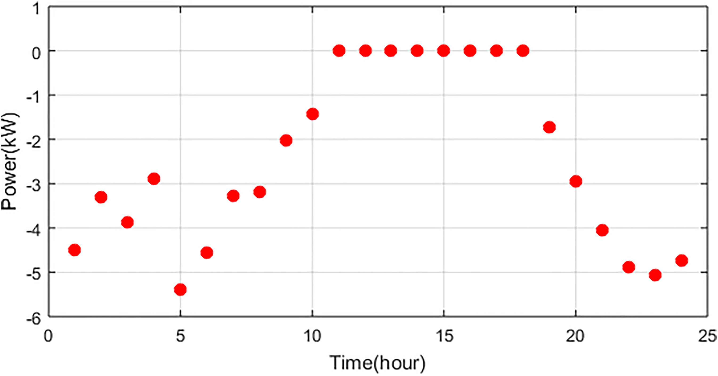
One-day power balance of summer for grid purchase.

One-day power balance of summer for photovoltaic (PV) power.

One-day power balance of summer for wind power.

One-day power balance of summer for grid sale.
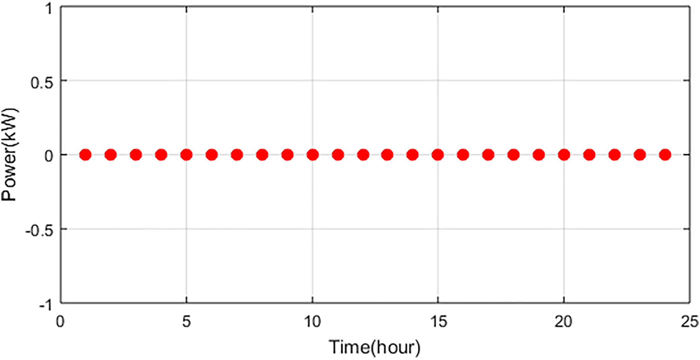
One-day power balance of summer for excess power.
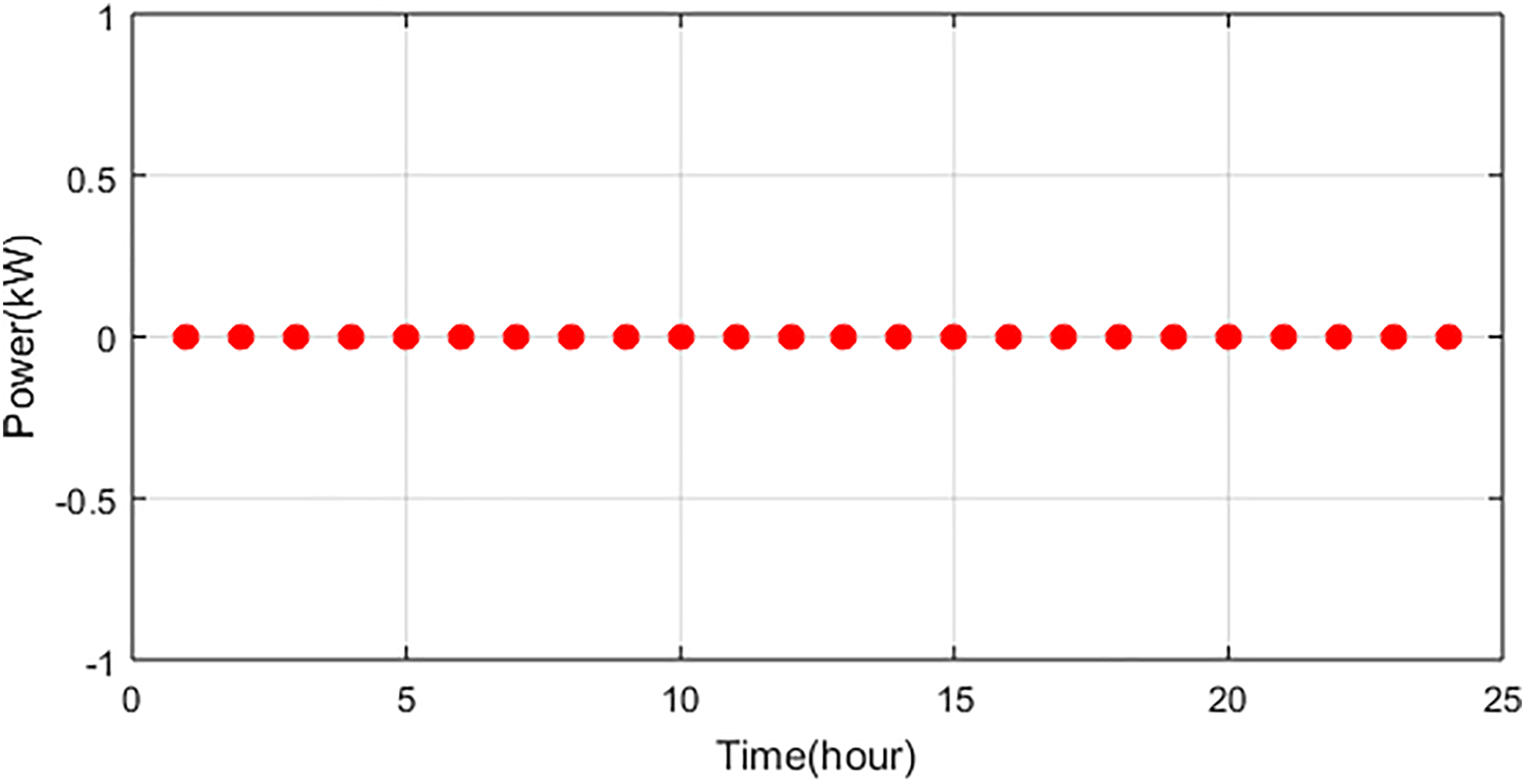
One-day power balance of summer for unmet load.
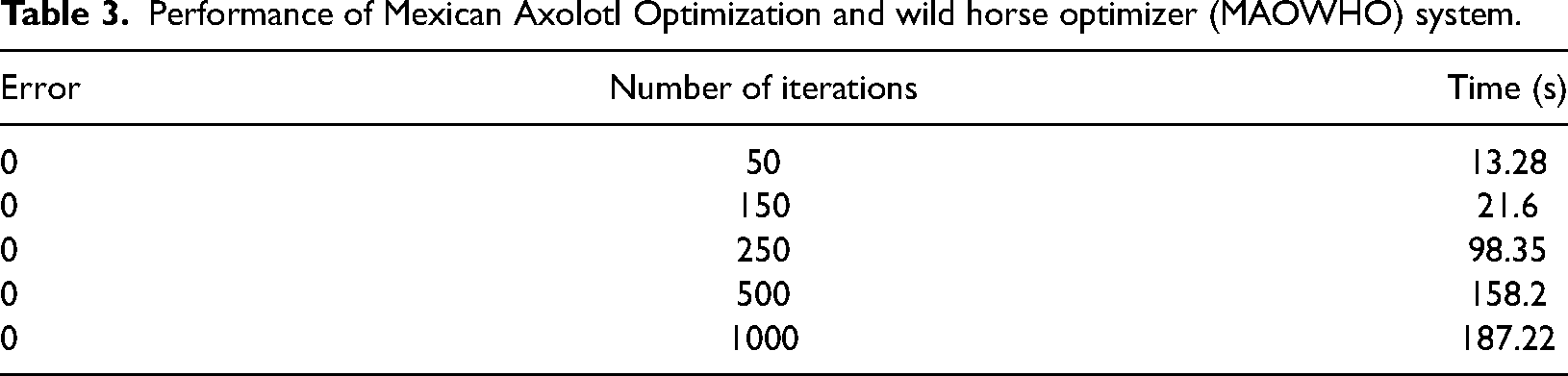
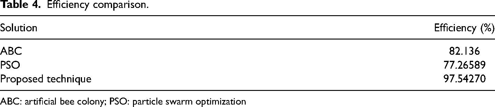
Table 1 depicts the convergence count of iterations and simulation time. Table 2 depicts the comparison of power consumption and system cost. Furthermore, Table 3 explained the performance of the proposed system. Table 4 depicts the efficiency comparison of solution techniques.
Convergence of count of iterations and simulation time.

Comparison of energy consumption and cost.

MAOWHO: Mexican Axolotl Optimization and wild horse optimizer; ABC: artificial bee colony; PSO: particle swarm optimization.
Performance of Mexican Axolotl Optimization and wild horse optimizer (MAOWHO) system.
Efficiency comparison.
ABC: artificial bee colony; PSO: particle swarm optimization
Conclusion
This paper proposes a hybrid method for grid-connected solar–wind hybrid system with EVs. Furthermore, the complexity is minimized by the proposed control scheme. The proposed control system is implemented on MATLAB/Simulink platform and its performance is evaluated. The results are compared to existing methodologies. The simulation outcomes demonstrate that EMS can lower total expenses in summer and winter related to conventional charging policy though ensuring the fulfillment rate of EV-charging demand in the absence of deliberate departure times of EVs. Finally, the sensitivity analysis impact of maximum grid sales and buy capabilities on LCOE is calculated. Finally, lower switching losses improve the efficiency of the proposed converter. Researchers should endeavor to improve available infrastructure device mechanisms in order to simplify future EV dispersion on roads and highways. More vehicles must be examined for intelligent power allocation strategies in the future, as well as various single and hybrid ways to assure higher fitness value and reduced computational time. The proposed method can be used to optimize CSs for EVs in remote regions, and it would make an interesting topic for further research.
Footnotes
Data availability statement
Data sharing does not relate to this article as no novel data has been formed or examined in this study.
Declaration of conflicting interests
The authors declared no potential conflicts of interest with respect to the research, authorship, and/or publication of this article.
Funding
The authors received no financial support for the research, authorship, and/or publication of this article.
