Impacts of climate and vegetation change on carbon accumulation in a south-central Alaskan peatland assessed with novel organic geochemical techniques

Abstract

To constrain the effect of climate and peatland type on carbon accumulation, we reconstructed these parameters from a Holocene-length core of a Sphagnum-dominated peatland near Cordova, AK, USA. We determined peat type using a combination of peat texture and density, macrofossils, distributions of leaf-wax biomarkers, and soil pH reconstructions based on distributions of branched glycerol dialkyl glycerol tetraether lipids (brGDGTs). We produced an independent record of hydroclimate and temperature change using hydrogen isotope ratios of leaf-wax biomarkers and distributions of brGDGTs. Carbon accumulation rates were constrained with 14 AMS ¹⁴C dates from identified macrofossils and ash-free bulk density. In the early Holocene, the site was a shallow pond with evidence for emergent macrophytes, Sphagnum, and algae growing in a warm, moist climate. At 9.2 kyr (1 kyr = 1000 cal. yr BP), the site became a Sphagnum-dominated bog. Under mid-Holocene warm, evaporative climate conditions, the site became sedge-dominated. As climate cooled and effective precipitation increased, Sphagnum was able to gain dominance abruptly at ~3.5 kyr. Large changes in the vegetation assemblage and hydrology and climate are contemporaneous with significant changes in the rate of carbon accumulation. Carbon accumulated most rapidly when Sphagnum dominated and effective moisture was high and most slowly when sedges were dominant and conditions were warmer and drier. Estimates of future climate change indicate warmer, more evaporative conditions that, in the past, favored a sedge-dominated environment, suggesting that this peatland and those similar can contribute to a positive feedback to warming by transitioning to less efficient carbon sinks.

Keywords

carbon cycle organic geochemistry paleoclimate paleoecology peatlands stable isotopes

Introduction

Northern peatlands are an important component of the global carbon cycle. While covering only 3% of Earth’s surface, peatlands can account for up to 30% of the carbon stored in terrestrial soils – a 550 Gt reservoir (Gorham, 1991; Roulet et al., 2007; Yu et al., 2010). Peatlands have been a major sink of atmospheric carbon throughout the Holocene, as the vast majority of the 550 Gt of carbon has accumulated since the end of the Pleistocene (Gorham et al., 2003). While these important ecosystems have been removing carbon from the atmosphere for millennia, their role in the carbon cycle may drastically change because of recent and future warming. Anthropogenic warming is expected to result in higher temperatures, longer growing seasons, increased precipitation, increased evaporation, and more episodic precipitation in the Arctic (Christensen et al., 2007). A detailed understanding of the response of peatlands to specific changes in climate is necessary to assess the impact that warming will have on peatlands and their role in the global carbon cycle (Beilman et al., 2009). However, we hypothesize that more episodic precipitation may result in a vegetation shift from a vegetation type that is more efficient at carbon sequestration (dominated by Sphagnum) to one that is less efficient, like sedges (Kuiper et al., 2014). Because Sphagnum photosynthetic rate is extremely sensitive to drying, if precipitation were to become more episodic, even if the total amount of precipitation were unchanged, Sphagnum would be at a disadvantage because of the periods of dryness in between episodes of precipitation (Williams and Flanagan, 1996). To assess the relative influence of these different factors – climate and vegetation type – on carbon accumulation, we reconstruct these parameters in the same samples from a Holocene-length core from a southern Alaskan peatland.

Typically, climate is reconstructed from peatlands using paleoecological techniques. However, if we are to disentangle the effects of vegetation and climate changes, we need to reconstruct climate independent of vegetation. We have chosen biomarker and compound-specific stable isotope methods to avoid this circularity. We used the hydrogen isotope ratios of leaf-wax biomarkers to assess changes in hydroclimate and temperature. Such measurements have come into common use recently, but their interpretation is complicated and depends on many site-specific parameters (Hou et al., 2008; Kahmen et al., 2013a, 2013b; Sachse et al., 2006; Smith and Freeman, 2006; Xie et al., 2000, 2004). To understand changes in temperature and peatland pH, we measured the distributions of branched glycerol dialkyl glycerol tetraether lipids (brGDGTs; Peterse et al., 2012; Weijers et al., 2007). By using these biomarker proxies, one is able to reconstruct climate and hydrological change independent of vegetation change.

Corser Bog, located at 60.5296364°N latitude and 145.453858°W longitude, is a Sphagnum peatland along the south-central Alaskan coast (Figure 1). The peatland can currently be classified as ombrotrophic (rain-fed) and Sphagnum-dominated, but because it is a local topographical high and surface flow directions are away from the peatland, even if the peatland itself was not always strictly ombrotrophic by chemical or vegetational definition, the topography of the site is such that the primary hydrologic input to the peatland is precipitation.

Figure 1.

Map of Corser Bog and its environs. An outline of the peatland (determined by walking the perimeter with a GPS device) is overlain on an orthophoto raster image. Inset shows the location of study site along the southern coast of Alaska. Two core locations are labeled in this figure. Core B was used for this investigation. Core A, which exhibits the same lithological units as Core B, is archived in the Lamont-Doherty Earth Observatory Core Repository. Inset: Summary of monthly climate and δD of precipitation at Cordova, AK. Dashed line indicates temperature; solid line indicates δD of precipitation calculated using the Online Isotopes in Precipitation Calculator (Bowen and Revenaugh, 2003; Bowen and Wilkinson, 2002; Bowen et al., 2005). Bars indicate precipitation amount in millimeters.

Average annual rainfall and temperature measured at the nearby Cordova airport, 15 km to the south, are 3 m and 4°C, respectively. Overall, the climatology of south-central Alaska, the region in which Corser Bog is found, is sensitive to the dynamics of the North Pacific Ocean. Precipitation is abundant throughout the year, but generally higher during August, September, and October. This early autumn peak in precipitation is because of increased cyclogenesis during this time of year driven by the Aleutian Low pressure system (Pickart et al., 2009). The temperature, precipitation, and cloudiness in south-central Alaska in general are highly sensitive to changes in sea surface temperatures in the North Pacific like the Pacific Decadal Oscillation (PDO; Hartmann and Wendler, 2005; Mantua et al., 1997).

Methods

Core collection and chronology

The 372 cm core was extracted from Corser Peatland with a 10-cm-diameter, tripod-mounted, modified Livingstone piston corer in five successive drives. The core was split in the Lamont-Doherty Earth Observatory Core Repository and imaged with a Geotek linescan camera. Core stratigraphy was determined by visual inspection of the core, magnified images, measurements of ash-free bulk density (AFBD), and the radiocarbon chronology.

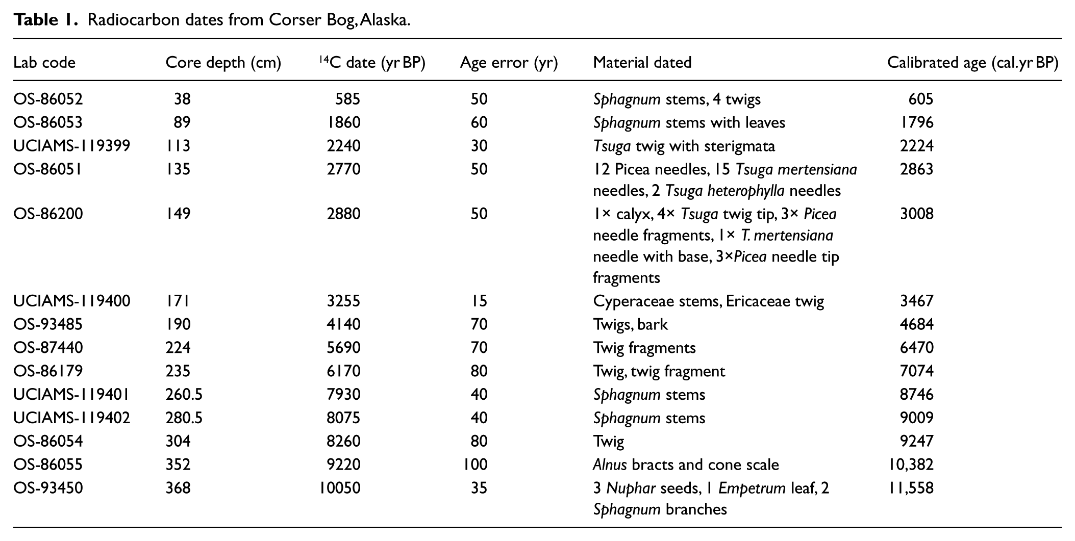
The age of the core is determined by 14 AMS radiocarbon dates on identified terrestrial macrofossils (Table 1). Dated material was separated from the peat by wet-sieving with a 500-µm screen and then pretreated with an acid–alkali–acid chemical digestion prior to combustion, graphitization, and measurement by AMS at the National Ocean Science Accelerator Mass Spectrometry Facility (Woods Hole, MA) or the W. M. Keck Carbon Cycle Accelerator Mass Spectrometry Laboratory (University of California, Irvine, CA).

Table 1.

Radiocarbon dates from Corser Bog, Alaska.

Lab code	Core depth (cm)	¹⁴C date (yr BP)	Age error (yr)	Material dated	Calibrated age (cal. yr BP)
OS-86052	38	585	50	Sphagnum stems, 4 twigs	605
OS-86053	89	1860	60	Sphagnum stems with leaves	1796
UCIAMS-119399	113	2240	30	Tsuga twig with sterigmata	2224
OS-86051	135	2770	50	12 Picea needles, 15 Tsuga mertensiana needles, 2 Tsuga heterophylla needles	2863
OS-86200	149	2880	50	1× calyx, 4× Tsuga twig tip, 3× Picea needle fragments, 1× T. mertensiana needle with base, 3×Picea needle tip fragments	3008
UCIAMS-119400	171	3255	15	Cyperaceae stems, Ericaceae twig	3467
OS-93485	190	4140	70	Twigs, bark	4684
OS-87440	224	5690	70	Twig fragments	6470
OS-86179	235	6170	80	Twig, twig fragment	7074
UCIAMS-119401	260.5	7930	40	Sphagnum stems	8746
UCIAMS-119402	280.5	8075	40	Sphagnum stems	9009
OS-86054	304	8260	80	Twig	9247
OS-86055	352	9220	100	Alnus bracts and cone scale	10,382
OS-93450	368	10050	35	3 Nuphar seeds, 1 Empetrum leaf, 2 Sphagnum branches	11,558

Carbon content

Carbon content in the core was determined using the AFBD of the peat measured by the loss-on-ignition (LOI) method. Volumetric samples (~2 cm³) of peat were dried at 100°C overnight to determine water content, and then burned in a muffle furnace at 550°C for 2 h to determine AFBD. AFBD is converted to carbon content by multiplying by 0.423 in Sphagnum peat and 0.514 in sedge peat (Loisel et al., 2014).

Organic and stable isotope geochemistry

Organic molecules were extracted from 36 freeze-dried peat samples by ultrasonic agitation in hexane. Each sample was approximately 0.5 g dry weight. Organic compounds were extracted by ultrasonic agitation. Samples were sonicated for 30 min in 20 mL of hexane three times. After each round of sonication, the extract was decanted from the beaker and replaced with another 20 mL of hexane. The products of each of these three successive rinses were combined for the total lipid extract (TLE). The TLE was separated into three fractions on a silica gel flash column. The flash column was prepared in a Pasteur pipette with a dimethylchlorosilane-treated glass wool plug and 5 cm of silica gel (60 Å pore size, 70–230 mesh). TLEs were loaded onto the column using 0.5 mL or less of hexane. Hydrocarbons were eluted from the column with 4 mL of hexane; ketone, ester, and aromatic compounds were eluted with 4 mL of dichloromethane; and polar compounds (including brGDGTs) were eluted with 4 mL of methanol.

n-Alkanes were analyzed in the Lamont-Doherty Earth Observatory Organic Geochemistry Laboratory. Relative abundances of n-alkanes (plant leaf waxes) were measured on a Thermo TraceGC with flame ionization detector. A pulsed temperature vaporization (PTV) injector, and a 30 m, HP-5 column were used. The oven temperature holds at 60°C for the first minute then ramps at 22°C/min to 200°C, and then ramps at 7.5°C/min to 320°C and holds for 10 min. Hydrogen isotope ratios of individual n-alkanes were determined by continuous flow isotope ratio mass spectrometry (Thermo TraceGC, GC-Isolink, ConFlo IV, Delta V IRMS). The GC injector, column, and temperature program are the same as for GC-FID described above. Eluent from the gas chromatograph is pyrolyzed to hydrogen gas in a high temperature furnace at 1430°C, which flows through the ConFlo IV continuous flow device to the IRMS. The median standard deviation for sample replicates is <1‰. Long-term standard deviation of repeated measurements of laboratory standards (mixture of fatty acid methyl esters) is ~2.5‰.

brGDGTs were analyzed in the Biogeochemistry Laboratory at the University of Massachusetts, Amherst. The methanol fractions from the above-described analyses were filtered through 0.45 µm PTFE syringe filters in 99:1 hexane:propanol (vol/vol) and analyzed on an Agilent 1260 HPLC coupled to an Agilent 6120 MSD (Hopmans et al., 2000; Schouten et al., 2007). A Prevail Cyano column (150 mm × 2.1 mm in surface area, and 3 µm of opening) was used with 99:1 hexane:propanol (vol/vol) as an eluent. After the first 7 min, the eluent increased by a linear gradient to 1.8% isopropanol (vol) over the next 45 min at a flow rate of 0.2 mL/min. Scanning was performed in selected ion monitoring (SIM) mode.

Results and discussion

Radiocarbon ages

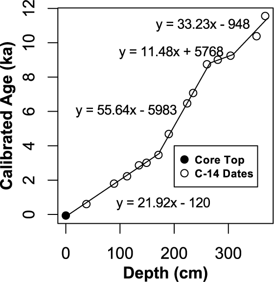
In all, 14 AMS radiocarbon measurements made on identified macrofossils constrain the chronology of the 372-cm-long core (Table 1). Dates were calibrated using the IntCal09 calibration dataset with the program Calib 6.1.0, and were reported as calibrated years before ad 1950. The top of the core is assigned an age of −60, corresponding to the date it was taken, July 2010. The age–depth model we have assigned consists of four linear sections (Figure 2). The mathematical intersections of adjacent age/depth functions coincide with changes in peat texture and AFBD described in the following sections.

Figure 2.

Radiocarbon age model from Corser Bog. Four linear regressions through the median calibrated ages calculated from Calib 6.1.0 and IntCal09 were used to distribute age throughout the core. Changes or breaks in slope of the age–depth model coincide with observed changes in peat type and density.

Core stratigraphy

Visual inspection of peat texture, LOI, AFBD, measurements, and the age–depth model (Figure 2) reveals five distinct periods of sediment accumulation over the 372 cm of the core (Figure 3). From the bottom of the core to 345 cm depth, LOI values are ~50%. Above 345 cm, the LOI sharply increases to between 80% and 90%. Radiocarbon sampling density is not sufficient to reveal strong evidence for a change in accumulation rate with this change in LOI (Figure 2), and we treat this section (372–302 cm) as one unit, Unit I. This unit is characterized by dark brown, faintly laminated, light-brown gyttja, interrupted by Alnus stems and roots and was deposited between 11.5 and 9.2 kyr.

Figure 3.

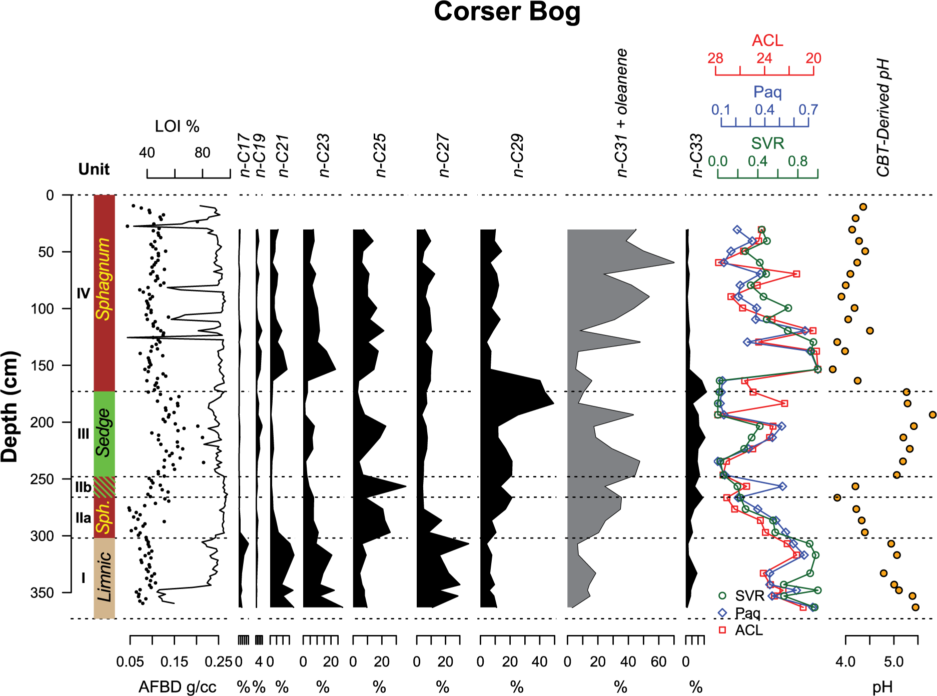
Downcore results from Corser Bog. From left to right: Unit designations used throughout the text, core lithology, percent LOI, fractional abundances of n-alkanes, n-alkane indices, and CBT-reconstructed pH. C₃₁ n-alkane coelutes with oleanene, an angiosperm triterpenoid, so a combined value is reported. Indices include the average chain length (ACL), P-aqueous ratio (P_aq), and the Sphagnum/Vascular Ratio (SVR).

Unit II, from 302 to 248 cm, is bounded at the bottom by a sharp contact between light-brown gyttja and fibrous Sphagnum peat and at the top by a drop in the LOI from values above 95% to as low as 80% (Figure 2). This unit contains two subunits, IIa and IIb. The contact between IIa and IIb is drawn at the change in AFBD at 266 cm (Figure 3), which coincides with a change in sedimentation rate (Figure 2). All of Unit II is characterized by LOI values consistently >95% in spite of the noticeable change in density at the IIa/IIb contact and was deposited between 9.2 and 7.8 kyr. However, the smoother texture and higher density of Unit IIb suggests it is more strongly decomposed than IIa, because sedges in the overlying unit, which are arenchymous, may have oxygenated this layer after it was deposited.

Unit III, from 248 to 173 cm, is bounded at the top and bottom by large changes in sedimentation rate (Figure 2), AFBD, and LOI (Figure 3) and is characterized by sedge-dominated peat with low accumulation rate, high AFBD, and LOI values between 80% and 95%. Unit III was deposited between 7.8 and 3.6 kyr. Unit IV, the top 173 cm of the core, consists of fibrous Sphagnum peat with LOI that is more consistently above 90%. In the upper 150 cm of the core, several sharp decreases in LOI are apparent with no visible change in the peat stratigraphy or density. These layers may be tephra or atmospherically derived dust.

Carbon accumulation

Carbon accumulation rates (CARs) are shown in Figure 4. In Unit I, in the gyttja, the median measured CAR is 14 g/m²/yr. Carbon accumulates fastest in the Sphagnum-dominated Unit IIa, where the median CAR is 27 g/m²/yr The lowest CAR values are found in the decomposed Unit IIb and the sedge-dominated Unit III, with median CARs 7.5 and 13 g/m²/yr, respectively. The rates calculated in these two units show the strong impact of the transition to sedge peat on the carbon storage. Not only does sedge peat accumulate less carbon over time but also promotes carbon loss in the peat directly below. Finally, the site transitions to Sphagnum-dominated peat in Unit IV, with median CAR of 20 g/m²/yr. We find that the CAR during the Sphagnum-dominated Units is about 60% higher (median = 21 g/m²/yr) than in the sedge-dominated Units (median = 13 g/m²/yr). The fact that the sedge-dominated environment is less efficient at sequestering carbon is consistent with plot-scale peatland manipulation experiments, for example (Kuiper et al., 2014).

Figure 4.

(a) Carbon density of peat samples (g/cm³); (b) Carbon accumulation rate (CAR; g/m²/yr); (c) Sphagnum/Vascular ratio (SVR) where values near 1 indicate abundant Sphagnum-derived n-alkanes and values near 0 indicate abundant vascular plant-derived n-alkanes; (d) MBT-/CBT-derived temperature estimates from Corser Bog using two different soils calibrations. Black bars above temperature data indicate approximate times of glacier advances for which evidence is apparent in south-central Alaska. (e) δD of C23 n-alkane (‰ VSMOW), (f) δD of C29 n-alkane, (g) Black diamonds indicate the most probable value for the δD of peatland water. The heights of the blue bars indicate the interquartile range of possible values, and the widths indicate the relative probability. Horizontal lines indicate the modern amount-weighted average values of δD of precipitation for June, July, August, and annually. The right-hand y-axis is a temperature axis scaled using the linear relationship between the monthly δD of precipitation and monthly temperature in Cordova. Black bars indicate glacier advances as in D. (h) Black diamonds indicate the most probable value for the evaporation index, ƒ. The heights of the red bars indicate the interquartile range of possible values, and the widths indicate the relative probability.

n-Alkane distributions

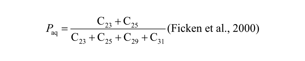
Distributions of n-alkane homologues in epicuticular waxes from plant leaves are an increasingly common data type used for paleoecological reconstruction. The relative abundances of the major constituents of the hydrocarbon fraction of the extracts from Corser Bog sediment samples are displayed in Figure 3. We also report several n-alkane indices: the average chain length (ACL), P-aqueous ratio (P_aq), and the Sphagnum/Vascular Ratio (SVR), all of which seek to reduce the many measurements of compound abundances in each sample to a single representative value. The ACL is equal to the sum of fractional abundance of each alkane multiplied by its carbon number. The P_aq ratio is equal to the fractional abundance of 23 and 25 carbon alkanes relative to 29 and 31 carbon alkanes. The SVR is a rescaling of the ratio of C₂₃ to C₂₉ n-alkane and represents the ratio of Sphagnum-derived alkanes relative to vascular plant-derived alkanes. The equations for each of the three indices are shown below:

A C L = \sum_{n = 17}^{33} n \times \frac{[C_{n} H_{n + 2}]}{[a l k a n e s]}

P_{a q} = \frac{C_{23} + C_{25}}{C_{23} + C_{25} + C_{29} + C_{31}} (Ficken et al ., 2000)

\begin{array}{l} S V R = - 0.0151 \times {(\frac{C_{23}}{C_{29}})}^{4} + 0.1144 \times {(\frac{C_{23}}{C_{29}})}^{3} - \\ 0.3916 \times {(\frac{C_{23}}{C_{29}})}^{2} + 0.8996 \times (\frac{C_{23}}{C_{29}}) - 0.0455 \\ (Nichols et al ., 2006) \end{array}

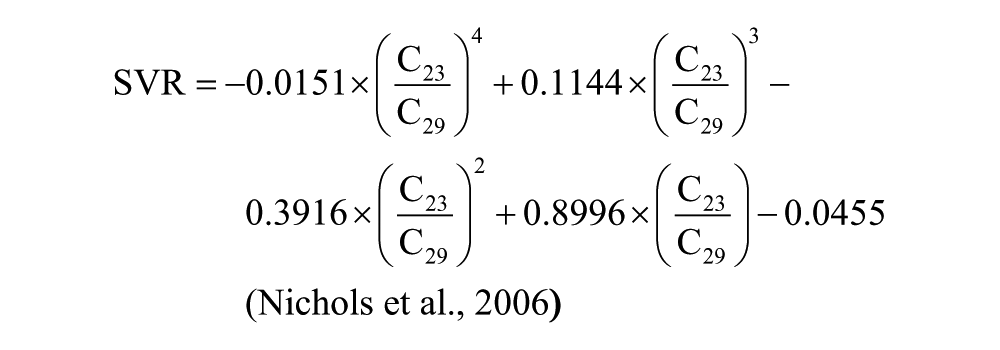
All three indices are highly correlated (Figure 3). We choose to use the SVR for our interpretation. It does not include C₃₁ n-alkane, which, in our samples, coelutes with olean-12-ene, a degradation product of olean-12-ene-3β-ol, a compound derived from angiosperms (Otto et al., 2005), and is therefore difficult to quantify. The SVR is based on the relative abundance of C₂₃ and C₂₉ n-alkane (Sphagnum and vascular plant biomarkers, respectively) and has been used to quantify the fraction of total alkanes contributed by Sphagnum relative to vascular plants (Nichols et al., 2006). Changes in SVR reflect the changes in the relative contribution of n-alkanes by Sphagnum and vascular plants, but this index underestimates the biomass input of Sphagnum to the sediment because total production of n-alkanes by Sphagnum is generally lower than that of vascular plants (Pancost et al., 2002). Consequently, even when SVR values are very low, such as in Unit III, Sphagnum can still be present and contribute to peat carbon. In Unit I, the SVR is above 0.4, indicating significant input from Sphagnum (Figure 3). The percent contribution of C₁₇ to total n-alkanes is also at its highest during this period. C₁₇ is typically a product of aquatic algae (Sachse et al., 2012). The coexistence of Sphagnum and aquatic algae supports the interpretation that this unit was deposited in a shallow pond environment. The Nuphar seed identified at 368 cm (Table 1) further supports this interpretation. Sphagnum remains an important part of the system through Unit II, as indicated by SVR values near 0.4. In Unit III, however, Sphagnum’s contribution to the peat is greatly reduced. The largest change in the record occurs at about 3.5 kyr, when the contribution of Sphagnum to the leaf-wax n-alkane pool changes from nearly 0 to nearly 1. This large change in SVR is concurrent with the transition from the sedge peat of Unit III to the Sphagnum peat of Unit IV. From its high at 3.0 kyr, the SVR declines through the remainder of the Holocene, but Sphagnum remains an important contributor to peat n-alkanes.

We find that CAR is higher when Sphagnum contributes a higher proportion of n-alkanes (Figure 4), but we do not see a direct correlation between SVR and CAR. Rather, when SVR indicates that the peatland is Sphagnum-dominated, CAR is higher than when SVR indicates that the peatland is not Sphagnum-dominated. For example, while SVR declines throughout the late Holocene, ~3.5–0 kyr, CAR remains relatively constant but higher than in the mid-Holocene, ~8–3.5 kyr, when SVR is very low and sedges dominate.

Hydrogen isotope ratios of n-alkanes

By measuring the hydrogen isotopes of individual leaf waxes, we assess both the deuterium isotopic composition (δD) of peatland water and the amount of evaporation occurring from Sphagnum during the growing season. We have used the δD of vascular plant biomarkers in peatland sediments to reconstruct the δD of peatland water as has been done previously (Nichols et al., 2009, 2010). δD of n-alkanes, however, is difficult to interpret. Here, we will discuss our approach to converting the δD of sedimentary alkanes into a climate signal. At high latitudes, temperature is the dominant control on the δD of precipitation, and Corser Bog is no exception (Figure 1). However, the range of values for the δD of C₂₉ n-alkane is 35‰. If we were to directly interpret δD of C₂₉ as temperature using the relationship between monthly δD of precipitation and monthly temperature, it would result in estimates of Holocene temperature change of about 10°C, which does not agree with the 3°C range in Holocene July temperatures estimated using pollen transfer functions in sediments from nearby peatlands (Heusser et al., 1985). To what, then, do we attribute the 35‰ range in δD of C₂₉? Hydrogen isotope ratios of C₂₉ n-alkane are determined not only by the δD of source water but also by the apparent fractionation factor between water and lipid (ϵ_w−l). It is the δD of source water that can potentially be influenced by temperature or other climatic or hydrologic factors. Thus, before interpreting these measurements, we must convert δD of alkanes using appropriate values of ϵ_w−l.

Variability of the apparent fractionation between water and lipid (ϵ_w−l) exerts a strong influence on the δD of sedimentary alkanes. For vascular vegetation, the factors determining ϵ_w−l are leaf water evaporation (Kahmen et al., 2013a, 2013b) and the plant type, which influences the biological fractionation (Sachse et al., 2012). While leaf water evaporation is a less important influence on ϵ_w−l in humid regions (Hou et al., 2008; Kahmen et al., 2013b), the difference in apparent fractionation between monocots, which dominate sedge peat, and dicots, which dominate the vascular vegetation in Sphagnum peat, is large – up to 40‰ (Sachse et al., 2012). The 35‰ range in δD of C₂₉ at Corser Bog could potentially be entirely because of changing vegetation type.

To better understand the variability in source water δD, that is, variability in climate and hydrology, we have translated the δD of C₂₉ into peatland water δD using apparent fractionation factors from a recent compilation (Sachse et al., 2012). In Sphagnum peat, we use ϵ_w−l values for dicots sampled from locations north of 45°N, and for samples in sedge peat, we use ϵ_w−l values for monocots found north of 45°N. Rather than simply using a mean value for ϵ_w−l, we account for the uncertainty in this parameter using the following method. For each lipid sample, we calculate the δD of water 10⁴ times, each time randomly choosing a value for ϵ_w−l from a probability distribution generated from the Sachse et al. (2012) compilation (Figure 5). The lithology of the core determines the distribution from which random ϵ_w−l are chosen – the monocot distribution is used for samples from sedge peat, and the dicot distribution is used for samples from Sphagnum peat and gyttja. The marked values for peatland water δD in Figure 4(g) represent the most probable δD value of peatland water.

Figure 5.

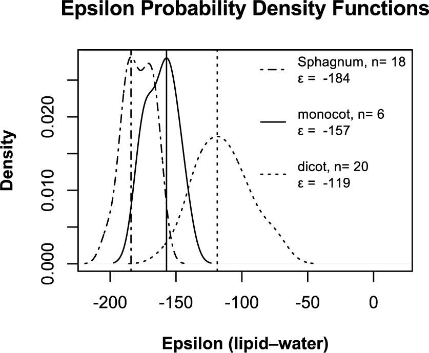
Probability density functions of ϵ_w−l for C₂₉ in dicotyledonous and monocotyledonous plants sampled from locations north of 45°N latitude (Sachse et al., 2012), and C₂₃ in Sphagnum sampled from various locations around the Laurentian Great Lakes (Nichols et al., 2010). Vertical lines indicate the most probable ϵ_w−l.

Particularly striking is the stark difference between the pattern of variability in the δD of C₂₉ record and the δD of water record. While δD of C₂₉ in Unit III is depleted relative to the other units, the most probable δD of water in this Unit is enriched relative to the other units. Comparing these two records illustrates the strong influence of vegetation type on δD of alkanes and the importance of independent reconstructions of vegetation to accompany measurements of alkane δD. Only after translating alkane δD values into source water δD values can we interpret changes in the record as having to do with changes in climate, hydrology, or other allogenic parameter.

A plant’s source water δD is determined by the δD of precipitation, precipitation seasonality, and soil water evaporation. With a topographically isolated watershed of <0.3 km², source water for plants living in this peatland, or ‘peatland water’, is dominated by precipitation. Corser Bog is topographically higher than the surrounding lakes, and thus is a source of water to the lakes. Because the seasonal range of δD of precipitation is so large, 65‰ (Figure 1), precipitation seasonality can have a strong influence on δD of peatland water (Nichols et al., 2009; Steig et al., 1994). Although the modern average monthly precipitation is relatively constant throughout the year, with a small peak in precipitation amount in autumn (Figure 1), this may not have always been the case. Depending on the residence time of peatland water, the source water for peatland vascular plants may have been dominated by spring melt, or by warm season precipitation. This variation would result in a source water δD value that could vary up to the seasonal range of 65‰. We find that during the late Holocene, ~3.5–0 kyr, the δD of peatland water is about equivalent to the modern average for δD of summer (JJA) precipitation, based on estimates from the Online Isotopes in Precipitation Calculator (OIPC; Bowen and Revenaugh, 2003; Bowen and Wilkinson, 2002; Bowen et al., 2005). This result is to be expected – the vascular plants in the peatland use water that fell as precipitation during the growing season. In the early Holocene, from about 11–9 kyr, peatland water transitioned from a value closer to modern average annual precipitation δD to a value closer to the summer precipitation value. During this time, the site was transitioning from a shallow pond environment into a Sphagnum peatland. As a pond with a potentially longer residence time, it is more likely that the water used by vascular plants was representative of the full year’s precipitation. As the site transitioned from a shallow lake to a peatland, the volume of water available to vascular plants decreased, thus shortening the residence time of that water. As a result, the δD of the peatland water as recorded by the vascular plants became more representative of the growing season average, rather than annual.

The δD of peatland water during the middle Holocene, however, cannot be explained by changing the seasonality of precipitation or hydrology of the site because the water values from 8 to 3.5 kyr are more enriched in deuterium than the current warm season precipitation. If we translate the enrichment in δD of peatland water into temperature using a linear relationship between monthly δD of precipitation and monthly temperature (Figure 1), we end up with a mid-Holocene that is ~4.5°C warmer than the late Holocene (Figure 4). This is a larger temperature change than was estimated using pollen transfer functions from nearby peatlands (Heusser et al., 1985). Heusser et al. (1985) estimated that July temperatures were about 3°C warmer than the late Holocene. This 1.5°C difference in temperature estimates of temperature change translates to 6‰ of δD change, which is within the uncertainty of our estimate of ϵ_w−l.

To estimate the amount of evaporation occurring at the peatland surface, we use a combination of the δD of Sphagnum and vascular plant biomarkers (C₂₃ and C₂₉ n-alkane respectively). Sphagnum, which has no vascular system, uses water found either in its hyaline cells or trapped between its leaves (referred to as ‘Sphagnum water’), that is strongly affected by evaporation at the surface of the peatland, while vascular plants use water from below the surface (referred to as ‘acrotelm water’) that is protected from evaporation (Kim and Verma, 1996; Nichols et al., 2010). The contrast in the δD of the biomarkers from these two groups can be used to estimate the amount of evaporation at the surface of the peatland (Nichols et al., 2010). Similar techniques, comparing the δD of terrestrial and algal n-alkanes, have been used in lake sediments (Mügler et al., 2008). We estimate the evaporation occurring at the surface of Corser Bog using the δD of C₂₃ and C₂₉ n-alkane according to the following method adapted from Nichols et al. (2010). We convert C₂₃ and C₂₉ n-alkane δD values into Sphagnum water and acrotelm water δD values using the above-described method of repeatedly choosing random ϵ_w−l value from probability distributions of ϵ_w−l (Figure 5). We then use the two most probable water δD values and a Rayleigh evaporation model to estimate the fraction of water remaining after evaporation (ƒ). Values of ƒ closer to 1 indicate more effective moisture, and values close to 0 indicate that Sphagnum is experiencing highly evaporative conditions. The equation for ƒ follows (Nichols et al., 2010) in the form of

f = e^{\frac{δ D a - δ D s}{ε_{k} + ε *}}

where δDa is the isotope ratio of peatland acrotelm water, δDs is the isotope ratio of Sphagnum water, ϵ_k is the kinetic enrichment factor at 0.75 relative humidity (3.125‰), and ϵ* is the equilibrium enrichment factor at 288 K (86.731‰).

A script defining functions to calculate ƒ from the δD of n-alkanes written in the open-source statistical programming language, R, is provided as Appendix 2, available online.

Using the n-alkane-derived values of ƒ, we find that the most evaporative part of the record occurs during the transition from Sphagnum peat to sedge peat just before ~8 kyr. Evaporative conditions, as indicated here by low values for ƒ, favor the growth of vascular plants as they can draw water from below, and need not rely on a constant supply of precipitation. Furthermore, groundwater can infiltrate the peatland against the gravitational hydrologic flow via transpiration by sedges, bringing nutrients that will support a change in vegetation from oligotrophic Sphagnum to mesotrophic sedges (Glaser et al., 1997), thus increased evaporation not only lowers water tables, allowing peat to oxidize, but also can facilitate vegetation change to species that are less efficient at storing carbon. The least evaporative part of the record, ~3 kyr, corresponds with coolest part of the Holocene, as well as the major transition from a sedge peatland to a Sphagnum peatland. As the evaporative stress is reduced and vapor pressure deficit decreases, vascular transpiration also reduces, halting the reverse flow of nutrient-rich groundwater, allowing Sphagnum to flourish, and restoring the peatland’s high capacity to store carbon.

Reconstructed pH and temperature

The methylation of branched tetraethers (MBT) and cyclization of branched tetraethers (CBT) are two relatively new proxies based on brGDGTs, lipids that are widespread in soils and peats (Weijers et al., 2007). brGDGTs are different in both the number of methyl branches (MBT) and the degree of cyclization (CBT). CBT varies as a function of soil pH while MBT varies as a function of mean annual temperature and to a lesser extent, soil pH. The use of these two proxies in combination, the MBT/CBT Index, allows for the influence of pH to be removed and for mean annual soil temperature to be reconstructed (Weijers et al., 2007). To date, the MBT/CBT proxy has mainly been applied to soils and lacustrine sediments (e.g. Fawcett et al., 2011; Tierney et al., 2012), while only a handful of studies have examined brGDGTs in peatlands (e.g. Ballantyne et al., 2010; Huguet et al., 2010; Weijers et al., 2011). A study of an ombrotrophic peat bog in Switzerland showed that brGDGTs in a peat core were mainly fossil lipids rather than derived from extant biomass (Weijers et al., 2011). Furthermore, the study of the Swiss peatland revealed a significant shift in CBT-reconstructed pH, coinciding with a stratigraphic change in peat composition from Carex-dominated, which formed in a fen system, to a Sphagnum-dominated peat. The Carex peat yielded CBT-reconstructed pH values of ~8, whereas the Sphagnum-dominated peat yielded lower values of ~4–5, as expected (Weijers et al., 2011). MBT/CBT temperatures based on the same samples yielded mean annual temperature (MAT) estimates within the standard error of the calibration (5°C) but possibly with a warm bias (Weijers et al., 2011). A warm bias has been noted at a few peat bogs and is often observed in soils, which may result from a combination of the insulating effect of vegetation and the heat capacity of (soil) water (Weijers et al., 2011). The combined effect is likely to be pronounced in peat bogs. Although the use of brGDGTs to reconstruct environmental conditions in peat bogs is fraught with potential complications related to the unknown origin of these compounds, which are thought to be produced by anaerobic soil bacteria (e.g. Sinninghe Damsté et al., 2011; Weijers et al., 2006), our results from Corser Bog lend support to the use of the MBT and CBT proxies for reconstructing past environmental conditions from peat bogs.

In Corser Bog, we find that the CBT-reconstructed pH of the peat is consistent with expected pH values in each peat type. CBT-reconstructed pH values in Unit I range from about pH 5.0–5.5 (Figure 3) – near the pH of rainwater, which would be expected in a rain-fed, non-carbonate pond. Units II and IV, the Sphagnum peat units, have CBT-derived pH values between 4.0 and 4.5 (Figure 3), consistent with Sphagnum-dominated bogs (Vitt, 1990). In Unit III, pH values are between 5.2 and 5.8 (Figure 3), more typical of sedge-dominated systems (Vitt, 1990).

MBT/CBT estimates of mean annual air temperature (MAT) were examined at Corser Bog using two available soil calibrations (Peterse et al., 2012; Weijers et al., 2007). While neither of these calibrations seems to reconstruct reasonable range of temperatures for the Holocene – both calibrations reconstruct a range of temperatures for the Holocene that exceeds 6°C – the shifts in temperature we reconstruct are broadly consistent with changes in glacial ice extent documented throughout south-central Alaska (Figure 6). This consistency suggests that the MBT/CBT temperature estimates, although incorrect in overall magnitude, may change in a manner consistent with Holocene temperature change. The warming start of the Holocene (Levy et al., 2004) is represented by the increase in temperature from ~11 to 9 kyr. The start of the Neoglacial is starkly apparent in the MBT-derived temperature record. At Corser Bog, the switch to cold temperatures occurs between 3.8 and 3.3 kyr. This is consistent with glacier advances dated to 3.7 (Calkin et al., 2001), 3.2 (Levy et al., 2004), and 3.6 kyr (Wiles and Calkin, 1994). We also record a rise in temperature at 2 kyr and a dip in temperature centered on 1.3 kyr that are concurrent with glacier retreats and advances, respectively, in the Prince William Sound region (Calkin et al., 2001).

Although there are clearly uncertainties associated with calibrating GDGT indices with temperature and perhaps also with pH, the general correspondence between changes in the MBT-/CBT-derived temperature estimates and the advance/retreat activity of glaciers in the region is an encouraging indication that the brGDGTs can be a valid tool for paleoclimate reconstruction in peatlands. As has been noted previously, further research will be required to determine whether the soil calibration is suitable for peat or whether a peat-specific calibration is required (Weijers et al., 2011). Well-constrained calibrations are especially necessary in sedimentary records with large changes in depositional environment, such as from lake to peatland, as at Corser. In any case, the consistency with which the GDGT-reconstructed pH corresponds with inferred pH based on peat type is an exciting indication that this proxy is useful in reconstructing the pH of peatland environments even while further work is needed to properly calibrate MBT/CBT.

Controls on carbon accumulation and abrupt ecological change

The early Holocene at Corser Bog was characterized by moist climate with lower rates of evaporation, evidenced by the growth of Sphagnum, and the maintenance of a shallow pond environment. The middle Holocene is warmer and drier than the early Holocene. Rates of evaporation are high, fostering the growth of a sedge dominance, which is less efficient for a carbon sink, compared with Sphagnum (Murray et al., 1989). The middle Holocene climate interpretation is consistent with the absence of glacial advances in south-central Alaska during the middle Holocene. Cooler, moister climate with lower evaporation rates prevails in the late Holocene, fostering Sphagnum growth and the transition from a sedge fen to a bog. This bog environment accumulates carbon 60% as rapidly as the sedge-dominated environment that preceded it.

Why should the transition from the sedge-dominated middle Holocene to the Sphagnum-dominated late Holocene be so abrupt, as our proxy evidence suggests? If climate is forcing vegetation change and responding to a slow insolation forcing, change should be gradual, but the transition from the middle to late Holocene is at the decadal scale. This could be because of the fact that sedge-dominated systems are self-supporting; sedges grow in tussocks with dense rhizomes that could crowd out Sphagnum, but provide substrate for other vascular species (Koyama and Tsuyuzaki, 2012); they also transpire more quickly than other types of vascular vegetation such as ericaceous shrubs, lowering the water table in the peatland and favoring species with deep root systems, that is, not Sphagnum (Murray et al., 1989). High rates of transpiration by sedges could also reverse the direction of hydrological flow, and potentially draw groundwater from the surrounding watershed into the peatland, providing nutrients that would otherwise not be available in a rain-fed system – higher nutrient availability also favors sedges over Sphagnum (Siegel and Glaser, 1987). If the growing season precipitation increases enough to ensure that the dominant flow in the peatland is out rather than in, the sedges would be cut off from their nutrient supply and Sphagnum, which thrives in low nutrients and high water tables will take over the peatland, producing the system we see today, significantly increasing the capacity of the peatland to accumulate carbon.

Conclusion

It is well known that the cool, moist Arctic and Sub-Arctic wetlands favor peat growth and carbon accumulation. Here, evidence from Corser Bog, Alaska, USA, elucidates some of the mechanisms by which climate and the hydrological cycle influence carbon accumulation. The direct influence of climate on carbon storage is moderated by climate’s influence on vegetation type. We found that carbon accumulates fastest when the site was a Sphagnum-dominated environment, and most slowly when it was a sedge-dominated environment. Units characterized by increased abundance of Sphagnum and low pH corresponded with times of cooler temperatures and reduced evaporation during the growing season. These moist, cool, ombrotrophic conditions encourage the growth of Sphagnum – an efficient peat former. Sedge-dominated units, with less acidic pH, corresponded with increased evaporative water loss and possible contribution of nutrient-rich groundwater during the growing season, fostering the growth of vascular species, particularly sedges – poorer peat formers. These results from Corser Bog also provide insight on the potential influence of recent and future climate change on carbon accumulation in this and similar systems. Because recent and future warming can result in climate conditions favorable to the sedge-dominated environment, Corser Bog and sites like it in boreal Alaska may act as a positive feedback for anthropogenic warming by transitioning to a type of environment that is less efficient at sequestering atmospheric carbon.

Footnotes

Acknowledgements

The authors would like to thank Philip Meyers and an anonymous reviewer for their helpful comments on the manuscript. The Prince William Sound Science Center in Cordova, Alaska, provided critical logistical support while collecting the Corser Bog core as well as area orthophotos and other geographical data.

Funding

This work is supported by the US National Science Foundation ARC-1022979 and by the Climate Center of the Lamont-Doherty Earth Observatory. JEN and CMM also gratefully acknowledge support from the NASA Postdoctoral Program and the US Geological Survey Mendenhall Postdoctoral Fellowship, respectively.

References

Ballantyne

Greenwood

Sinninghe Damsté

. (2010) Significantly warmer Arctic surface temperatures during the Pliocene indicated by multiple independent proxies. Geology 38: 603–606.

Beilman

MacDonald

Smith

. (2009) Carbon accumulation in peatlands of West Siberia over the last 2000 years. Global Biogeochemical Cycles 23(1): GB1012.

Bowen

Revenaugh

(2003) Interpolating the isotopic composition of modern meteoric precipitation. Water Resources Research 39(10). DOI: 10.1029/2003WR002086.

Bowen

Wilkinson

(2002) Spatial distribution of δ18O in meteoric precipitation. Geology 30(4): 315–318.

Bowen

Wassenaar

Hobson

(2005) Global application of stable hydrogen and oxygen isotopes to wildlife forensics. Oecologia 143(3): 337–348.

Calkin

Wiles

Barclay

(2001) Holocene coastal glaciation of Alaska. Quaternary Science Reviews 20: 449–461.

Christensen

Hewitson

Busuioc

. (2007) Regional climate projections. In: Solomon

Qin

Manning

. (eds) Climate Change, 2007: The Physical Science Basis. Contribution of Working Group I to the Fourth Assessment Report of the Intergovernmental Panel on Climate Change. Cambridge: Cambridge University Press, pp. 847–940.

Fawcett

Werne

Anderson

. (2011) Extended megadroughts in the southwestern United States during Pleistocene interglacials. Nature 470(7335): 518–521.

Ficken

Swain

. (2000) An n-alkane proxy for the sedimentary input of submerged/floating freshwater aquatic macrophytes. Organic Geochemistry 31: 745–749.

10.

Glaser

Siegel

Romanowicz

. (1997) Regional linkages between raised bogs and the climate, groundwater, and landscape of north-western Minnesota. Journal of Ecology 85: 3–16.

11.

Gorham

(1991) Northern peatlands: Role in the carbon cycle and probable responses to climatic warming. Ecological Applications 1(2): 182–195.

12.

Gorham

Janssens

Glaser

(2003) Rates of peat accumulation during the postglacial period in 32 sites from Alaska to Newfoundland, with special emphasis on northern Minnesota. Canadian Journal of Botany 81: 429–438.

13.

Hartmann

Wendler

(2005) The significance of the 1976 Pacific climate shift in the climatology of Alaska. Journal of Climate 18(22): 4824–4839.

14.

Heusser

Peteet

(1985) Late-quaternary climatic change on the American North Pacific coast. Nature 315(6019): 485–487.

15.

Hopmans

Schouten

Pancost

. (2000) Analysis of intact tetraether lipids in archaeal cell material and sediments by high performance liquid chromatography/atmospheric pressure chemical ionization mass spectrometry. Rapid Communications in Mass Spectrometry 14(7): 585–589.

16.

Hou

D’Andrea

Huang

(2008) Can sedimentary leaf waxes record D/H ratios of continental precipitation? Field, model, and experimental assessments. Geochimica et Cosmochimica Acta 72(14): 3503–3517.

17.

Huguet

Fosse

Laggoun-Defarge

. (2010) Occurrence and distribution of glycerol dialkyl glycerol tetraethers in a French peat bog. Organic Geochemistry 41: 559–572.

18.

Kahmen

Schefus

Sachse

(2013a) Leaf water deuterium enrichment shapes leaf wax n-alkane δD values of angiosperm plants I: Experimental evidence and mechanistic insights. Geochimica et Cosmochimica Acta 111(C): 39–49.

19.

Kahmen

Hoffmann

Schefuß

. (2013b) Leaf water deuterium enrichment shapes leaf wax n-alkane δD values of angiosperm plants II: Observational evidence and global implications. Geochimica et Cosmochimica Acta 111(C): 50–63.

20.

Kim

Verma

(1996) Surface exchange of water vapour between an open Sphagnum fen and the atmosphere. Boundary-Layer Meteorology 79(3): 243–264.

21.

Koyama

Tsuyuzaki

(2012) Mechanism of facilitation by sedge and cotton-grass tussocks on seedling establishment in a post-mined peatland. Plant Ecology 213(11): 1729–1737.

22.

Kuiper

Mooij

Bragazza

. (2014) Plant functional types define magnitude of drought response in peatland CO2 exchange. Ecology 95(1): 123–131.

23.

Levy

Kaufman

Werner

(2004) Holocene glacier fluctuations, Waskey Lake, northeastern Ahklun Mountains, southwestern Alaska. The Holocene 14(2): 185–193.

24.

Loisel

Beilman

. (2014) A database and synthesis of northern peatland soil properties and Holocene carbon and nitrogen accumulation. The Holocene. DOI: 10.1177/0959683614538073.

25.

Mantua

Hare

Zhang

. (1997) A Pacific interdecadal climate oscillation with impacts on salmon production. Bulletin of the American Meteorological Society 78(6): 1069–1079.

26.

Mügler

Sachse

Werner

. (2008) Effect of lake evaporation on δD values of lacustrine n-alkanes: A comparison of Nam Co (Tibetan Plateau) and Holzmaar (Germany). Organic Geochemistry 39(6): 711–729.

27.

Murray

Harley

Beyers

. (1989) Water content effects on photosynthetic response of Sphagnum mosses from the foothills of the Philip Smith Mountains, Alaska. Oecologia 79(2): 244–250.

28.

Nichols

Booth

Jackson

. (2006) Paleohydrologic reconstruction based on n-alkane distributions in ombrotrophic peat. Organic Geochemistry 37(11): 1505–1513.

29.

Nichols

Booth

Jackson

. (2010) Differential hydrogen isotopic ratios of Sphagnum and vascular plant biomarkers in ombrotrophic peatlands as a quantitative proxy for precipitation – Evaporation balance. Geochimica et Cosmochimica Acta 74(4): 1407–1416.

30.

Nichols

Walcott

Bradley

. (2009) Quantitative assessment of precipitation seasonality and summer surface wetness using ombrotrophic sediments from an Arctic Norwegian peatland. Quaternary Research 72(3): 443–451.

31.

Otto

Simoneit

BRT

Rember

(2005) Conifer and angiosperm biomarkers in clay sediments and fossil plants from the Miocene Clarkia Formation, Idaho, USA. Organic Geochemistry 36(6): 907–922.

32.

Pancost

Baas

van Geel

. (2002) Biomarkers as proxies for plant inputs to peats: An example from a sub-boreal ombrotrophic bog. Organic Geochemistry 33(7): 675–690.

33.

Peterse

van der Meer

Schouten

. (2012) Revised calibration of the MBT–CBT paleotemperature proxy based on branched tetraether membrane lipids in surface soils. Geochimica et Cosmochimica Acta 96: 215–229.

34.

Pickart

Moore

GWK

Macdonald

. (2009) Seasonal evolution of Aleutian low pressure systems: Implications for the North Pacific subpolar circulation. Journal of Physical Oceanography 39(6): 1317–1339.

35.

Roulet

Lafleur

Richard

. (2007) Contemporary carbon balance and late Holocene carbon accumulation in a northern peatland. Global Change Biology 13(2): 397–411.

36.

Sachse

Billault

Bowen

. (2012) Molecular paleohydrology: Interpreting the hydrogen-isotopic composition of lipid biomarkers from photosynthesizing organisms. Annual Review of Earth and Planetary Sciences 40(1): 221–249.

37.

Sachse

Radke

Gleixner

(2006) δD values of individual n-alkanes from terrestrial plants along a climatic gradient – Implications for the sedimentary biomarker record. Organic Geochemistry 37(4): 469–483.

38.

Schouten

Huguet

Hopmans

. (2007) Analytical methodology for TEX86 paleothermometry by high-performance liquid chromatography/atmospheric pressure chemical ionization-mass spectrometry. Analytical Chemistry 79(7): 2940–2944.

39.

Siegel

Glaser

(1987) Groundwater flow in a bog-fen complex, Lost River Peatland, northern Minnesota. Journal of Ecology 75: 743–754.

40.

Sinninghe Damsté

Rijpstra

WIC

Hopmans

. (2011) 13,16-dimethyl octacosanedioic acid (iso-diabolic acid), a common membrane-spanning lipid of Acidobacteria subdivisions 1 and 3. Applied and Environmental Microbiology 77: 4147–4154.

41.

Smith

Freeman

(2006) Influence of physiology and climate on δD of leaf wax n-alkanes from C3 and C4 grasses. Geochimica et Cosmochimica Acta 70(5): 1172–1187.

42.

Steig

Grootes

Stuiver

(1994) Seasonal precipitation timing and ice core records. Science 266(5192): 1885–1886.

43.

Tierney

Schouten

Pitcher

. (2012) Core and intact polar glycerol dialkyl glycerol tetraethers (GDGTs) in Sand Pond, Warwick, Rhode Island (USA): Insights into the origin of lacustrine GDGTs. Geochimica et Cosmochimica Acta 77: 561–581.

44.

Vitt

(1990) Growth and production dynamics of boreal mosses over climatic, chemical and topographic gradients. Botanical Journal of the Linnean Society 104(1–3): 35–59.

45.

Weijers

JWH

Bernhardt

Peterse

. (2011) Absence of seasonal patterns in MBT-CBT indices in mid-latitude soils. Geochimica et Cosmochimica Acta 75: 3179–3190.

46.

Weijers

JWH

Schouten

Hopmans

. (2006) Membrane lipids of mesophilic anaerobic bacteria thriving in peats have typical archaeal traits. Environmental Microbiology 8: 648–657.

47.

Weijers

Schouten

van den Donker

. (2007) Environmental controls on bacterial tetraether membrane lipid distribution in soils. Geochimica et Cosmochimica Acta 71(3): 703–713.

48.

Wiles

Calkin

(1994) Late Holocene, high-resolution glacial chronologies and climate, Kenai Mountains, Alaska. Geological Society of America Bulletin 106(2): 281–303.

49.

Williams

Flanagan

(1996) Effect of changes in water content on photosynthesis, transpiration and discrimination against ¹³CO₂ and C¹⁸O¹⁶O in Pleurozium and Sphagnum. Oecologia 108(1): 38–46.

50.

Xie

Nott

Avsejs

. (2000) Palaeoclimate records in compound-specific delta D values of a lipid biomarker in ombrotrophic peat. Organic Geochemistry 31(10): 1053–1057.

51.

Xie

Nott

Avsejs

. (2004) Molecular and isotopic stratigraphy in an ombrotrophic mire for paleoclimate reconstruction. Geochimica et Cosmochimica Acta 68(13): 2849–2862.

52.

Loisel

Brosseau

. (2010) Global peatland dynamics since the Last Glacial Maximum. Geophysical Research Letters 37(13): L13402.