Multiproxy approach for Holocene paleoenvironmental reconstructions from microorganisms (testate amoebae and foraminifera) and sediment analyses: The infilling of the Loire Valley in Nantes (France)

Abstract

Foraminifera and testate amoebae are jointly used with sediment characteristics (sediment size, calcium carbonate, C, H, N and S proportions, and clay mineralogy) to reconstruct the Holocene sediment infilling of the Loire estuary (Nantes, France). The results reveal the infilling of the Loire Valley during the Holocene. Deposited on the Hercynian substratum, the first deposits are made of gravels with rare associated fauna. This corresponds to the gravel lag usually present as basal deposits in the river course. The clay mineralogy indicates an erosion of the substratum. Then, from 8850 to 5850 cal. yr BP, estuarine fauna settled in a laminated sediment that alternates between clay and sand. The smectite associated with kaolinite and illite suggests increased input from the Sèvre Nantaise River. The fauna progressively shifts from estuarine to marine, indicating a rise in the sea level. From 5850 cal. yr BP, the pace of the sea level rise slowed and channels migrated, implying intense erosion. After 2100 cal. yr BP, the fauna was dominated by testate amoebae, indicating a continentalization of the environment. The top samples reflect recent human activity and urbanization.

Keywords

foraminifera Holocene paleoenvironmental reconstructions sediment infilling testate amoebae

Introduction

Foraminifera (Rhizaria) and testate amoebae (Rhizaria and Amoebozoa) are unicellular eukaryotes, and are abundant and diversified in all modern aquatic and marine environments (Lee et al., 2000). Foraminifera are the best known and the most diversified of all microfossils (Sen Gupta, 1999). They are widely distributed in all marine and transitional marine environments (Murray, 2006; Scott et al., 2001), and play a significant role in global biogeochemical cycles of inorganic and organic compounds (Haynes, 1981; Lee and Anderson, 1991). It is well known that the composition, species diversity and spatial distribution of benthic foraminiferal assemblages are greatly controlled by environmental parameters (Hayward et al., 2004; Murray, 2006). Indeed, numerous environmental factors influence the distribution of foraminifera, including salinity (Gehrels et al., 2001), organic matter (OM) quality (Armynot du Châtelet et al., 2009) and sediment texture (Armynot du Châtelet et al., 2010; Magno et al., 2012).

Testate amoebae are ubiquitous and live in various freshwater environments. In particular, they are well developed in peat lands, rivers, lakes or brackish-water settings (Charman, 2001). Rare species can survive in brackish waters (Van Hengstum et al., 2008; Vazquez Riveiros et al., 2007). They also have the following advantages: high species diversity, widespread distribution, and the ability to tolerate extreme conditions (Beyens and Chardez, 1995) and/or react quickly to environmental change (Booth et al., 2004). Testate amoebae distribution is controlled by salinity (Gehrels et al., 2001; Van Hengstum et al., 2008). Other parameters also affect the development of testate amoebae communities, such as pollution (Nguyen-Viet et al., 2008) and seasonal variables like temperature, light penetration, primary production and precipitation (Neville et al., 2010).

Foraminifera are currently used to reconstruct marine paleoenvironments (Armynot du Châtelet et al., 2005; Edwards and Horton, 2000; Leorri et al., 2010), and testate amoebae are utilized in the same way as a common tool for freshwater paleoenvironmental reconstruction (Asioli et al., 1996; Charman, 2001; Ellison, 1995; Medioli and Scott, 1988; Wall et al., 2010). Meanwhile, in transitional environments (e.g. those with salinity constraints), a combination of both foraminifera and testate amoebae has been used in historical studies to reproduce environments of the past (Duleba and Debenay, 2003; Eichler et al., 2004; Gehrels et al., 2001; Lloyd, 2000).

An extensive study over about 15 worldwide estuaries published in 2006 (Dalrymple, 2006) indicates that, following the Zaitlin et al. (1994) model, most of the late Pleistocene–Holocene estuaries experienced severe changes in sediment fluxes during the overall rising sea level system. Most estuaries first present a transgressive unit prograding shoreward followed by a seaward prograding Highstand System Tract (HST; Dalrymple, 2010). French estuaries (whose Loire estuary), follow this general trend (Chaumillon et al., 2010; Proust et al., 2010). Numerous paleoenvironmental studies have examined the fossil fluvial valleys preserved on continental shelves. It is also the case that various approaches have been used all around the Bay of Biscay: seismic survey (Chaumillon et al., 2010; Menier, 2003; Proust et al., 2010), core drilling (Sorrel et al., 2010; Traini et al., 2013), or a combination of seismic/sedimentological/bio-indicator tools (Perez-Belmonte, 2008; Poirier, 2010). Nevertheless, no study has examined the continental parts of these valleys.

Using a multiproxy approach (sediment and faunal characteristics), the main objective of this research is to reconstruct the evolution of the environmental deposits during the Holocene sea level rise in the Loire upper estuary. This study allows a better understanding of the estuarine microfaunal response during the Holocene transgressive, which could be of importance for other worldwide paleoenvironmental studies.

Study area

The Loire River drains a watershed of 115,000 km² and flows into the Atlantic Ocean in the widely developed continental shelf of the Bay of Biscay. The Loire estuary extends over 100 km from Ancenis (upper limit for the tidal wave) to Saint-Nazaire (Figure 1). The flow rate ranges from 80 to 5500 m³/s (850 m³/s on average; Etcheber et al., 2007), while the turbidity reaches 3 g/L and the tidal prism is 3 × 10⁹ m³ (Etcheber et al., 2007). The seawater intrusion reaches 65 km upstream (Ciffroy et al., 2003b), and the turbidity maximum zone constitutes a stock of 1.5 × 10⁶ tons of fine particles with a residence time between 4 and 10 months. The sedimentation rate ranges from 0.5 cm/year upstream close to the Island of Nantes to 4 cm/year downstream close to Le Pellerin (Ciffroy et al., 2003b). During the Holocene, the thickness of the accumulated sediments was ca. 30 m near Nantes and ca. 40 m close to the river mouth in Saint-Nazaire (Ottmann et al., 1968; Ters et al., 1968).

Figure 1.

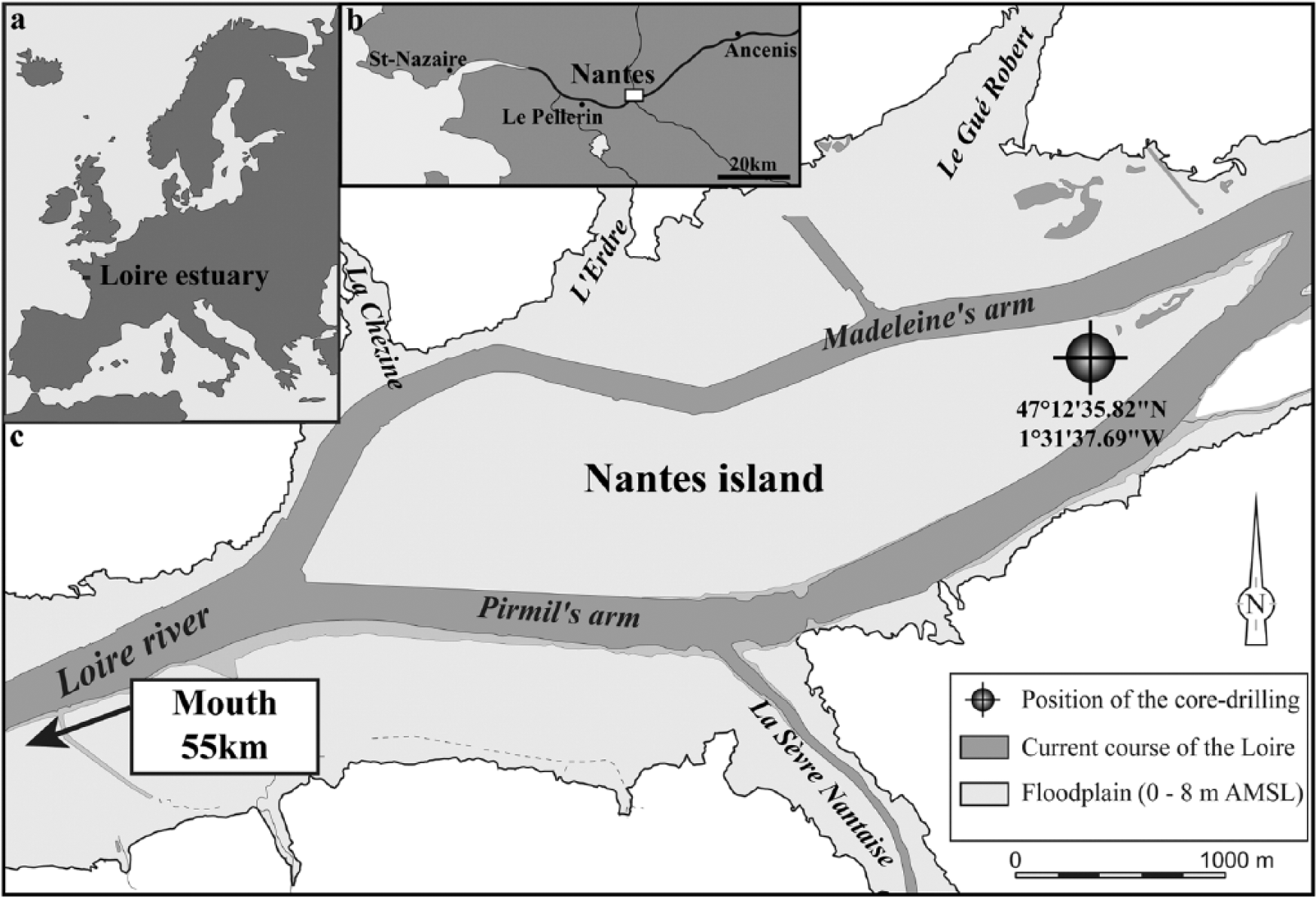
Localization of the study site in the European Atlantic coast (a) Loire estuary and (b) position of the core drilling at the eastern extremity of the (c) Nantes Island. AMSL (elevation above mean sea level, relative to the average sea level datum: NTF, ellipsoid Clarke 1880 IGN).

The spatial extent of the flood plain is controlled by the lithology and the Hercynian substratum structure. The Loire River watershed is composed of Paleozoic (Hercynian) metamorphic and magmatic bedrock and Mesozoic to Cenozoic sedimentary formations (Proust et al., 2010; Thinon et al., 2008). The northern part of the watershed is composed of altered granites, shales and gneiss that provide both illite and kaolinite (Delfau and Le Berre, 1981; Esteoule-Choux, 1967). The southern part of the watershed is composed of sand and sandy marl from which smectite is derived, and altered amphibolite and gabbros that provide vermiculite and other clay minerals (Esteoule-Choux, 1967).

The larger extension of the estuary is bordered by a tidal marsh and a tidal flat. The Nantes area is characterized by an island that is built from Hercynian headland. This so-called Nantes Island is 4.9 km long and 1 km wide. It is surrounded by two river channels: the Madeleine channel to the north and the Pirmil channel to the south (Figure 1). The area is now widely urbanized.

Material and methods

The core and the sampling

The core is situated close to Nantes Island (Figure 1). It was selected from nine cores drilled for a Collective Research Program (PCR Loire) that took place from 2010 to 2013. These cores were positioned following the inventory of the sedimentary deposits preserved within the Loire valley (Arthuis and Nauleau, 2008). This inventory is based on the 1586 core drillings carried out and compiled by The French geological survey (Bureau de Recherches Géologiques et Minières) in the area (available online at http://infoterre.brgm.fr/). The drilling was conducted with a swindler with a piston corer, and produced cores that are 1.5 m long with a 10 cm diameter. The total length is 30 m (the longest core in the area) and reaches the Hercynian substratum.

The core is located on the ancient channel of the Loire River and consequently records most of the sediment deposits that occurred throughout the Holocene. Two sets of sediment samples were selected: (1) 177 samples were chosen for the sediment grain size analyses, and (2) of these, 50 were also subjected to microfaunal analyses, calcium carbonate content, C and N elemental analyses, and a clay mineralogy analysis. The second set of samples was selected according to clayey and silty sediment grain size, which is more suitable for larger foraminiferal database and subsequent interpretation in estuaries (e.g. Armynot du Châtelet et al., 2009).

Sediment analyses

Sediment grain size

As a first step, the sediment grain size was eye-estimated to define the stratigraphic column and the lithologic units. Next, the 177 selected samples were analysed using the principle of diffraction of a monochromatic laser beam on suspended particles (Malvern Mastersizer 2000, red He–Ne laser, 632 and 466 nm wave lengths). This method is detailed by Trentesaux et al. (2001). Measurements can range from 0.02 to 2000 µm, with an obscuration of between 10% and 20%. A maximum of two modes were determined and used as descriptive parameters. Grains were grouped into six size classes: clay (<2 µm), fine silt (2–10 µm), sortable silt (10–63 µm), fine and very fine sand (63–250 µm), medium sand (250–500 µm), and coarse and very coarse sand (>500 µm).

Calcium carbonate

The calcium carbonate content was determined from 1 g of finely crushed bulk sediment using a Bernard calcimeter. The proportions are expressed as a dry sediment weight. Measurements were taken in triplicate for each sample. Reproducibility was good and all the three measurements were processed as a mean.

OM

The quantity and quality of the OM was approximated by estimating the total organic carbon (TOC) and N content in the sediment. This technique used a FlashEA 1112 Elemental Analyser (Thermo) and is explained in a former study performed in a similar environment by Armynot du Châtelet et al. (2009). The analysis was performed on 1.5–2 mg of sample added to approximately 5 mg of vanadiumpentoxide, used as a combustion catalyst. 2,5-bis(5-tert-butyl-benzoxazol-2-yl)thiophene (BBOT) was used as standard. The TOC content was then determined by subtracting the carbonate carbon (deduced from the calcium carbonate proportion) from the total C. Measurements were taken in duplicate for each sample and a mean was calculated after checking that there was no dissimilarity. An estimation of the OM quality was determined with the TOC/N ratio. Fresh OM from microalgae, which are protein-rich and cellulose-poor, has atomic TOC/N values that are commonly between 4 and 10, whereas vascular land plants, which are protein-poor and cellulose-rich, create OM that usually has TOC/N ratios of 20 and greater (Meyers, 1994). The proportions of OM that originate from these two general sources can consequently be distinguished by their TOC/N ratios.

Clay mineralogy

The clay mineralogy was used to trace the origin of the sediment in the estuary. The protocol used for clay mineralogy analyses is the classic procedure described by Bout-Roumazeilles et al. (1999). The analyses were run on a Brucker Endeavor D4 diffractometer coupled with a LynkEye detector between 2.49° and 32.5°. Each clay mineral was then characterized by its layer plus interlayer interval as revealed by an XRD analysis (Brindley and Brown, 1980). The semi-quantitative estimation of the abundances of the various clayey minerals is based on peak areas and added together to obtain 100% (smectite + illite + vermiculite + mixed-layers + chlorite + kaolinite = 100%). The error on the reproducibility of the measurements is estimated to be <5% for each clay mineral, as checked by an analysis of replicate samples.

Microfaunal analysis

The 50 samples (~20 cm³ each) were wet sieved through 38, 63, 125 and 315 µm mesh sieves. Five samples were used to identify the size fraction corresponding to the size of the fauna. Rare specimens are present in the 38–63 µm fraction. As a consequence, the study’s focus is on the 63–315 µm fractions. Within these fractions, terrigenous grains on the one hand and foraminifera and testate amoebae on the other were separated by flotation on trichloroethylene (d = 1.46 g/cm³). A detailed control of the residue of three test samples (the latter described as harbouring a rich fauna) was used to validate the methods: no foraminifera or testate amoebae were found in these residues.

Microfaunal observation, extraction and determination were carried out under a binocular Olympus SZX16 with a maximum magnification of 115. The taxonomic references used for the testate amoebae were: Leidy (1879), Ogden and Hedley (1980), Cash and Hopkinson (1905), Lee et al. (2000) and Clarke (2003). For the foraminifera, the taxonomic references were: Brady (1884) and Cimerman and Langer (1991). Only the species present as a proportion of at least 5% of at least one sample were selected for the statistical analyses. This procedure allowed us to remove the rare species.

The testate amoebae and foraminifera were classified into eight ecological groups (EGs): freshwater, tidal channel under a continental influence, salt marsh, tidal flat, tidal channel, marine infralittoral, marine circalittoral, and widespread estuarine species. The marine infralittoral group was subdivided into four sub-groups: epiphytes, dysoxic/anoxic tolerant infauna, OM rich and low O₂ content tolerant infauna/epifauna, and opportunist oxic epifauna. The ecological groupings are based on the work of: Severin (1983), Jones and Charnock (1985), Bernhard (1986), Corliss and Chen (1988), Duleba et al. (1999) and Goubert et al. (2001).

Radiocarbon dating

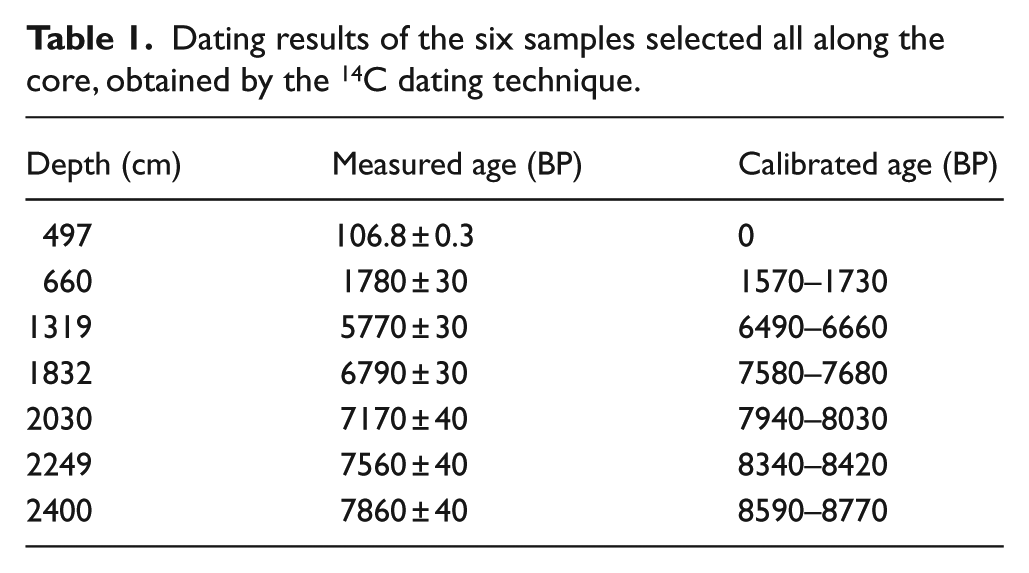
Six levels were dated by the ¹⁴C dating method. The maximal interval between two dated samples was 6.6 m. The samples were processed in the Beta Analytic laboratory and AMS-dated (classical dating of the short lived single-component materials which have been well preserved within the sediment).

The dates obtained were used to calculate an age–depth model, which was produced using the Bacon (Blaauw and Christen, 2011) approach: age–depth modelling uses Bayesian statistics to reconstruct Bayesian accumulation histories for deposits. The age-model was computed using the WinBacon package for the R software. The radiocarbon ages were converted to calendar ages using IntCal13 (Reimer et al., 2013). The age–depth model obtained was then discussed in light of the results obtained from the sediment and faunal characteristics.

Statistical analysis

The contingency, proportion and density were calculated based on microfaunal counting. The diversity index ( $H'$ – Shannon–Weaver index) was calculated as follows (Eq. 1):

H' = - \sum_{i = 1}^{s} p_{i} {log}_{2} p_{i}

(1)

where i is the species and $p_{i}$ is species proportions compared with the total number of species.

All of the biological and sedimentological data were treated with the integrated suite R (R-Development-Core-Team, 2014) with the following packages: Base (descriptive statistics), Vegan (diversity calculation), Rioja (construction of diagrams with timescale), Bacon (Blaauw and Christen, 2011; age–depth modelling).

Results

Lithology and sediment characteristics

Lithology, grain size and dating

The total length of the drilling was 30 m (Figure 2a). The top 4.5 m is composed of clearings and was not studied further. The base of the core (from 30 to 26.70 m) comprises gravely sediment, followed by coarse to fine sand (from 26.70 to 24.2 m). These levels are grouped in Section F₁. Another section with coarse sediment is also observed from 12.2 to 7.2 m (Section F₃), while laminated sediment with sizes ranging from clayey-silt to fine sand are observed (Section F₂) between these two sections. Three intervals with fine grain size sediments are observed in Section F₂ (between 22.3 and 21 m, 19.5 and 18.2 m, and then 13.9 and 12.9 m). The top section (from 7.2 to 4.5 m), meanwhile, is initially laminated and then the grain size rapidly decreases in size, reaching clayey-silt (Section F₄).

Figure 2.

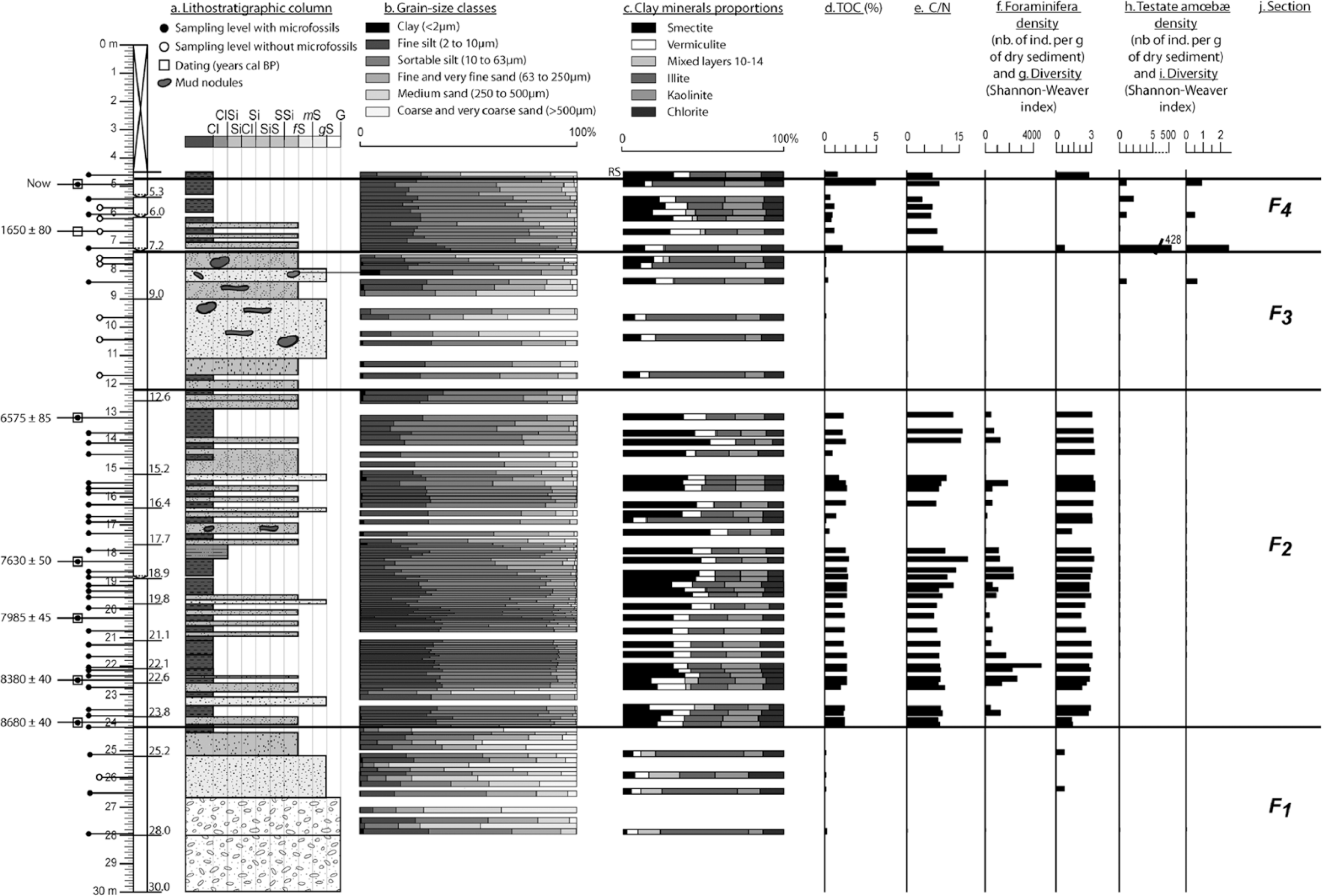
Along core analyses: (a) reconstitution of the lithostratigraphic column, (b) proportion of the grain size classes (Cl: clay, ClSi: clayey-silt, SiCl: silty clay, Si: silt, SiS: silty sand, SSi: sandy silt, fS: fine sand, mS: medium sand, gS: gravelly sand, G: gravels), (c) clay mineral proportions, (d) total organic carbon (TOC in %), (e) TOC/N ratio, (f) foraminifera density (number of individuals per gram of dry sediment), (g) foraminifera diversity (Shannon–Weaver index), (h) testate amoebae density (number of individuals per gram of dry sediment), (i) testate amoebae diversity (Shannon–Weaver index), and (j) the four sections (F₁ to F₄) of the evolution of the Nantes Island environment.

The 177 core sediment analyses revealed that the grain size ranges from clay to sand (Figure 2b). A total of 94 samples (more than 50% of the total sample) have mixed sand–silt–clay and clayey-silt sediment. A total of 18 samples are sand in size and 19 are clayey-sand. No pure clay sediments were measured.

A total of 41 samples present a bi-modal distribution. The coarsest mode ranges from 123 to 554 µm, while the fine particle mode ranges from 8.5 to 57 µm. The ¹⁴C ages (Table 1) are stratigraphically consistent and indicate that the sediments are Holocene in age, with a maximum age of 8770 cal. yr BP at a depth of 24.0 m.

Table 1.

Dating results of the six samples selected all along the core, obtained by the ¹⁴C dating technique.

Depth (cm)	Measured age (BP)	Calibrated age (BP)
497	106.8 ± 0.3	0
660	1780 ± 30	1570–1730
1319	5770 ± 30	6490–6660
1832	6790 ± 30	7580–7680
2030	7170 ± 40	7940–8030
2249	7560 ± 40	8340–8420
2400	7860 ± 40	8590–8770

Clay mineralogy

Six clay minerals were observed: smectite, illite, kaolinite, chlorite, vermiculite, and mixed-layers 10–14 (Figure 2c and Supplementary Data 1, available online). The chlorite proportion is almost constant throughout the core (13% ± 2%). The other clay minerals are grouped into three associations distributed along the core as follows:

Between the bottom of the core to 24.2 m, the clay fraction is dominated by illite (~45%), associated with mixed-layers and kaolinite. The vermiculite and smectite proportions are small (~7% and ~5%, respectively). This association corresponds to Section F₁.

Between 24.2 and 12.2 m, smectite is dominant (~35%) and associated with illite (~21%) and kaolinite (~18%). The mixed-layer mineral proportions are small (less than 9%). This association corresponds to Section F₂.

Between 12.2 and 4.5 m, higher proportions of illite (~37%) and kaolinite (~20%) are observed than in the underlying sections. These dominant minerals are associated with smectite (~18%). This clay mineral association corresponds to Sections F₃ and F₄.

OM quality and quantity

The TOC is variable and ranges from 0% to 5% (Figure 2d). Almost no TOC (0.12%) is measured in the lowest section of the core. This corresponds to Section F₁, with the coarsest sediments. All along the second section with coarse sediment (F₃), the TOC proportions are slightly higher, but never exceed 1%. In Section F₂, the sediment contains a mean TOC of 1.78%. A total of 33 samples (~80%) have a detectable proportion of N and enable the C/N ratio to be calculated (Figure 2e). The C/N ranges from 4.28 at 5.45 m to 17.33 at 18.32 m. For most of the sample, the C/N ranges from 9 to 12.

Microfaunal analysis

Microfaunal content

Among the 50 selected samples, 41 contained specimens of foraminifera and/or testate amoebae. A total of 10,726 individuals were extracted and identified at a species level: 10,384 are foraminifera and 342 testate amoebae. These specimens belong to 71 species of foraminifera and 23 species of testate amoebae. The main species are illustrated in Figures 3 –6. The counting is set out in Supplementary Data 1, available online.

Figure 3.

Anaglyphic (online coloured version only) SEM (scanning electron microscope) pictures showing foraminifera diversity of Nantes Island (1/2). 1: Remaneica plicata (50 μm); 2: Miliolinella subrotunda (50 µm); 3: Globulina minuta (50 µm); 4: Adelosina longirostra (50 µm); 5: Quinqueloculina seminula (100 µm); 6: Homalohedra williamsoni (100 µm); 7: Favulina scalariformis (50 µm); 8: Lagena cf. sulcata (50 µm); 9: Hyalinonetrion cf. clavatum (100 µm); 10: Lagena gracilis (100 µm); 11: Lagena sulcata spirata (50 µm); 12: Lagena sulcata (50 µm); 13: Vasicostella sp. (100 µm); 14: Astacolus crepidulus (50 µm); 15: Fissurina cf. semimarginata (50 µm); 16: Fissurina semimarginata (50 µm); and 17: Parafissurina sp. (50 µm).

Figure 4.

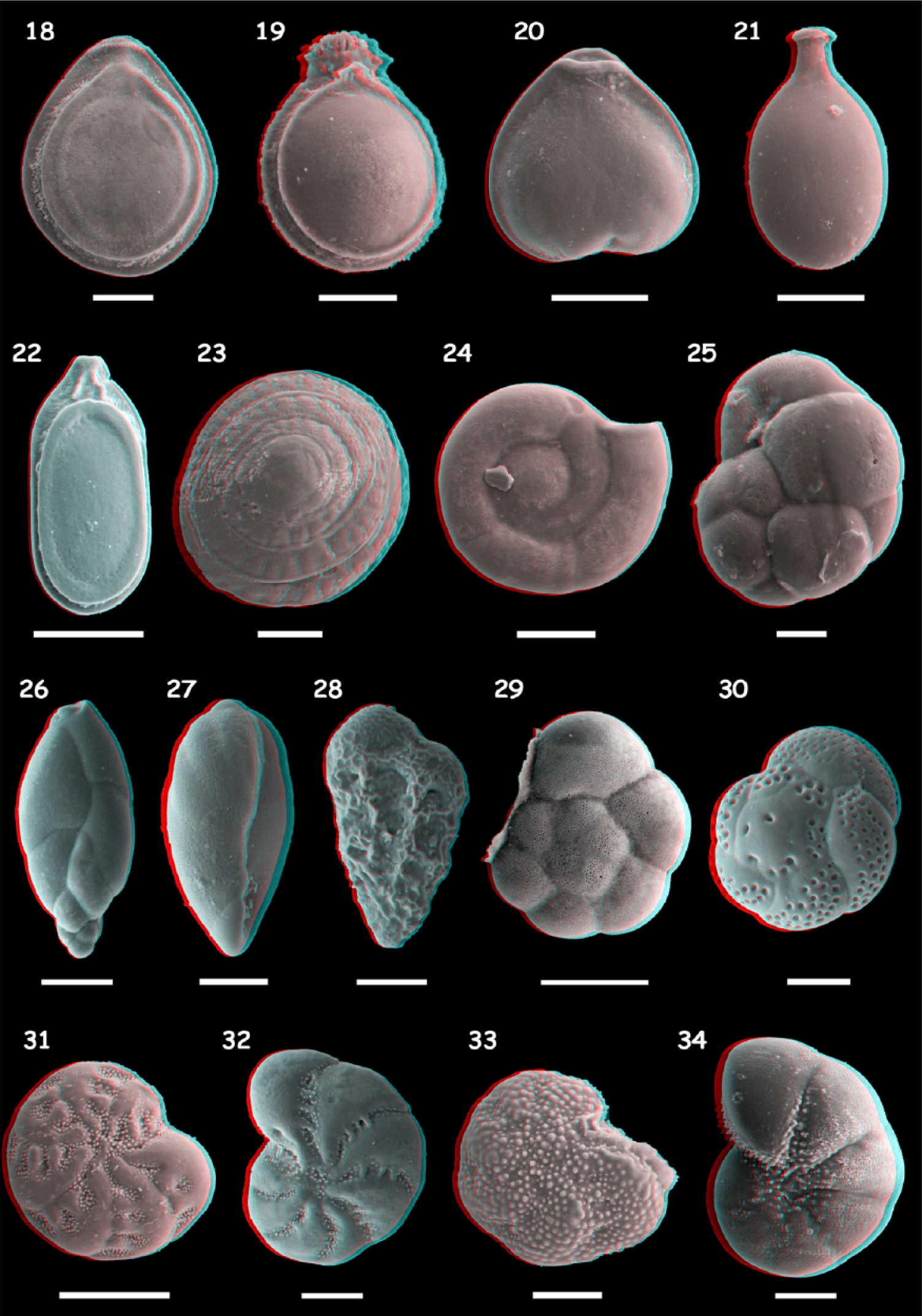
Anaglyphic (online coloured version only) SEM (scanning electron microscope) pictures showing foraminifera diversity of Nantes Island (2/2). 18: Fissurina fasciata carinata (50 µm); 19: Paliolatella orbignyana (50 µm); 20: Lagenosolenia plena (50 µm); 21: Lagenosolenia seguenziana (50 µm); 22: Lagenosolenia lagenoides (100 µm); 23: Patellina corrugata (50 µm); 24: Cornuspira involens (50 µm); 25: Cassidulina crassa (20 µm); 26: Stainforthia fusiformis (50 µm); 27: Bulliminella elegantissima (50 µm); 28: Bolivina pseudoplicata (50 µm); 29: Ammonia tepida (100 µm); 30: Rosalina bradyi (50 µm); 31: Elphidium earlandi (100 µm); 32: Cribroelphidium gerthi (50 µm); 33: Cribroelphidium margaritaceum (50 µm); and 34: Haynesina germanica (50 µm).

Figure 5.

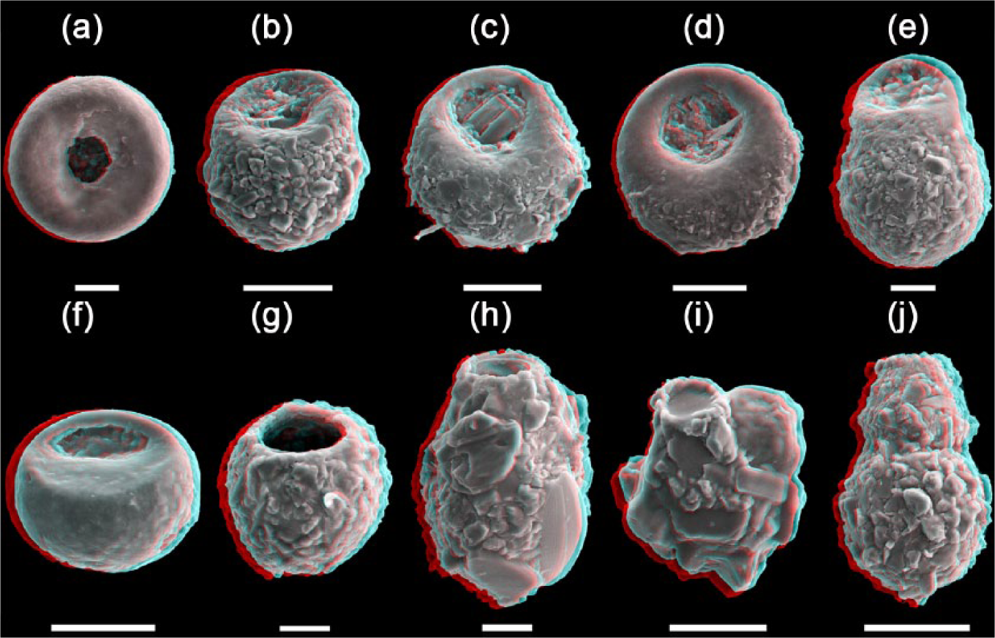
Anaglyphic (online coloured version only) SEM (scanning electron microscope) pictures showing testate amoebae diversity of Nantes Island. (a): Cyclopyxis kahli (20 µm); (b): Centropyxis aerophila (50 µm); (c): Centropyxis aculeata (50 µm); (d): Centropyxis ecornis (50 µm); (e): Centropyxis lobostoma (20 µm); (f): Plagiopyxis declivis (50 µm); (g): Difflugia globulosa (20 µm); (h): Difflugia cf. tenuis (20 µm); (i): Difflugia sp. (50 µm); and (j): Pontigulasia sp. (50 µm).

Figure 6.

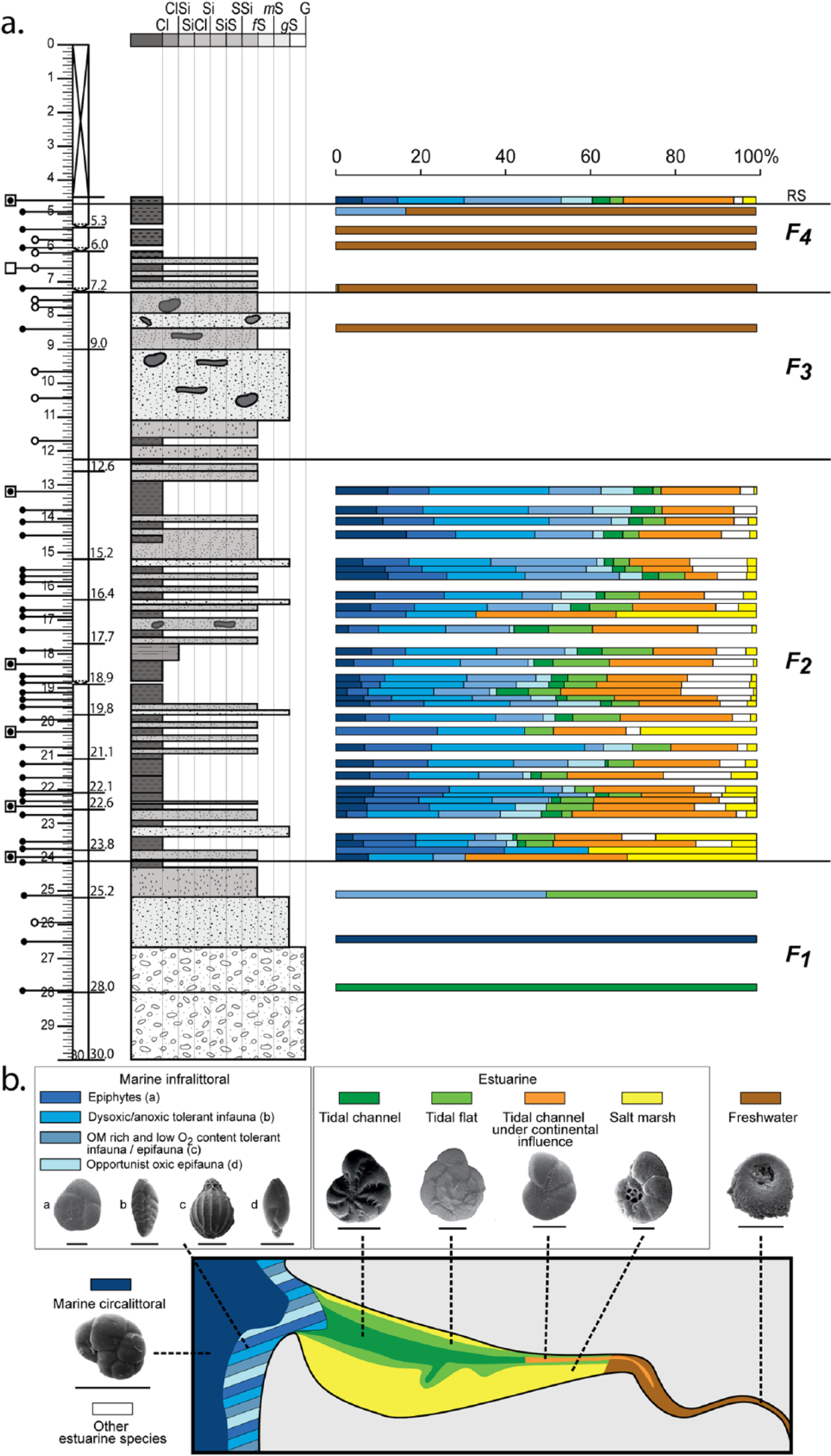
Diagram of the evolution of the microfauna composition (a) subdivided into ecological groups from freshwater to marine circalittoral and (b) their geographical distribution within an estuary. Most of the key species are illustrated (see text legend of Figures 3 –5). Scale bar of the SEM pictures = 100 µm.

The density of the foraminifera is highly variable along the core, ranging from 0 to 4600 specimens per gram of sediment (Figure 2f). No faunas are observed in the two coarsest sediment sections, F₁ and F₃. Three levels of high density are observed: from 22.7 to 21.6 m, 19.8 to 18 m, and at around 16.0 m. Testate amoebae are only observed in the upper section of the core between 8.4 m and the top (Figure 2h). The highest density reaches 428 individuals per gram of sediment (at 7.2 m). The mean density for the other samples where testate amoebae occur is 1.25 specimens per gram of sediment. Save for only one sample, the levels where testate amoebae occur correspond to the levels with an absence of foraminifera.

The diversity of the foraminifera ranges from 0 to 3.3 (Figure 2g), while that of the testate amoebae ranges from 0 to 2.5 (Figure 2i). This diversity is high for the foraminifera between 24.2 and 12.2 m (Section F₂), but is lower before and after that section. One sample close to 17.7 m has slightly lower diversity compared with its neighbouring samples. The top sediment sample reveals a great diversity of foraminifera, reaching 2.8. The diversity of the testate amoebae (above 8.5 m) reached 2.5 in only one sample at 7.20 m.

Haynesina germanica, with 20% of the total counted foraminifera, is the most common species. The other most frequent foraminifera species are as follows: Ammonia tepida (7.8%), Brizalina variabilis (7.5%), Bolivina pseudoplicata (7.4%) and Fissurina lucida (7.1%). The most frequent testate amoebae species are as follows: Centropyxis constricta (29.7%), Centropyxis aerophila (9.6%), Centropyxis aculeata (7.5%), Difflugia sp. (7.2%), Cyclopyxis kahli (6.9%) and Centropyxis ecornis (6.9%).

Ecological groups

The foraminifera and testate amoebae species are subdivided into eight EGs (Supplementary Data 2, available online): freshwater, tidal channel under continental influence, salt marsh, tidal flat, tidal channel, marine infralittoral, marine circalittoral, and widespread estuarine species. The marine infralittoral group has been further subdivided into four sub-groups: epiphytes, dysoxic/anoxic tolerant infauna, OM rich and low O₂ content tolerant infauna/epifauna, and opportunist oxic epifauna. The tidal channel under continental influence, salt marsh, tidal flat and tidal channel groups are all estuarine EGs.

The EGs evolve over time and are grouped into three periods (Figure 6). The Sections F₁, F₃ and F₄ are composed of only one or two EGs, whereas Section F₂ comprises all of the EGs but with variations in their relative proportions. The estuarine EGs are dominant at the bottom of the section. Moving up to 20.3 m, the proportion of the marine EGs increases (from 23% to 63%). Then, from 20.3 to 16.88 m, an alternation of the dominance of estuarine (mainly salt marsh and tidal channel under continental influence) and marine dominated EGs is observed. The samples at 20.3 and 16.88 m reveal an exceptionally high proportion of the tidal channel under continental influence EG. From 16.88 m up to the upper sample of this section, the proportion of each EG is roughly constant, with the marine EGs dominating (more than 56%) in association with the salt marsh EG. This increase in the proportion of the marine EG is due to the rise in the amount of the marine circalittoral and dysoxic/anoxic tolerant infauna EGs.

The highest proportion of the epiphytic EG is always associated with the highest percentage of the salt marsh and tidal channel under continental influence EGs.

Section F₄ comprises only the freshwater EG that is characterized by testate amoebae. The uppermost samples (RS in Figure 6) have an association of EGs that are similar to those described in the section ‘Study area’.

Interpretation and discussion

Environmental evolution versus faunal preservation

Large and diversified foraminifera assemblages have been described all along the core, whereas testate amoebae only occur in the upper section. The easiest explanation is an environmental change that caused a shift from a marine to a continental environment. This shift from foraminifera to testate amoebae is the same used by Lloyd (2000) for an Holocene environmental reconstruction. Moreover, Gehrels et al. (2001) observed that the vertical range of testate amoebae in salt marshes is small, attributed to a strong correlation with environmental changes. Duleba and Debenay (2003) specified, not surprisingly, that salinity was the main stress factor, which introduced the shift between foraminifera and testate amoebae. Nevertheless, the poor preservation of testate amoebae in the deepest sections could be also envisaged. In our study, the largely dominant genera Difflugia and Centropyxis (dominant as well in Lloyd’s (2000) study, and associated with two other agglutinated genus, Phryganella and Pontigulasia) are constituted of agglutinated shells, composed of minerals from the surroundings and cemented by an organic lining. Thanks to this strong structure (Armynot du Châtelet et al., 2013; Ogden and Hedley, 1980), they have a good chance of being preserved. In contrast, the Arcella and Euglypha genera, which are far less abundant, may be dissolved (Mitchell et al., 2008; Ooms et al., 2011; Swindles and Roe, 2007) or degraded because of sediment dehydration (Roe et al., 2002). As a consequence, they would not be well preserved in a fluvial environment such as the Loire estuary. A large diversity of a testate amoebae shell type could only be correctly preserved in a calm environment such as a lake (Wall et al., 2010). As a consequence, both environmental evolution and faunal preservation are responsible for testate amoebae changes throughout the core. The most robust testate amoebae shells (agglutinating forms) would be the only ones adapted for past environmental reconstruction in such a dynamic environment.

Agglutinated and calcareous foraminifera could also be prone to dissolution (Boltovskoy and Wright, 1976) and mechanical deterioration in coarse sediment (Armynot du Châtelet et al., 2009). In the present study, foraminifera are observed in all of the sections. Only the coarse sediment grains sections have logically lower densities. Within the other sections, the foraminifera are well preserved with a great diversity and density that makes them of high value for environmental reconstruction purposes.

Evolution of environment – OM and sediment size constraints

In a study of surface sediments from Skagerrak and Kattegat (Scandinavia), Alve and Murray (1999) showed that there is no obvious relationship between sediment grain size, organic content and the composition of foraminifera assemblages. In contrast, Armynot du Châtelet et al. (2009) in the Canche estuary (English Channel, Northern France) evidenced that both sediment grain size and total organic content appear to be limiting factors. In the present study, critical thresholds such as those defined by Murray (2001) are often reached all along the core. For example, both density and diversity are very low along the sections with the coarsest sediments (F₁ and F₃). These sections reflect high-energy environments that may inhibit OM sedimentation and favour the washing of bacteria biofilms or algal mats. Such environmental conditions prevent foraminifera from feeding, settling and developing in accordance with the strategy described by Murray (1986) and Schönfeld (2002).

All along the section (F₂), the clayey, silty and sandy layers rapidly alternate. Diversity and density (and the number of EGs) are high in this section. As a consequence, such tidal sediment layers do not limit the development of foraminifera and testate amoebae.

The second limiting factor may be the OM content and its quality, as depicted by the TOC proportion and the C/N ratio. Fresh OM from microalgae, which are protein-rich and cellulose-poor, has atomic C/N values that are commonly between 4 and 10, whereas vascular land plants, which are protein-poor and cellulose-rich, create OM that usually has C/N ratios of 20 and greater (Meyers, 1994). The proportions of OM that originate from these two general sources can consequently be distinguished by their C/N ratios. The average C/N value of the OM present in the core is intermediate between the two end-members (4.28 and 17.33), and therefore indicates a mixed contribution from algae and higher plants. Within the intermediate section, the C/N values indicate that OM derived as well from algae and higher plants. Through the interpretation of this proxy, pulses of continentalization or return of marine conditions alternatively could be evidenced. Nevertheless, the occurrence of N-rich layers between 6500 and 1650 yr BP may reflect as well early agriculture activities, as it has been observed through pollen evidence in close areas (Visset et al., 2001, 2002) and in Europe (Jalut, 1995; Lopez-Garcia and Lopez-Saez, 2000; Puertas, 1997; Richard, 1994). Finally, in the upper part of the core, the C/N values are low and may reflect algae influence. However, as these sediments are the most recent, an increase of agriculture influence cannot be excluded and the use of N-rich fertilizers may be responsible for the decrease in the C/N ratio observed. As a conclusion, C/N probably reflects episodes of continentalization throughout the core, with a specific anthropogenic influence in the most recent part of the record.

In the intermediate part of the core, the highest biological densities are associated with the highest C/N values. Even if the highest C/N cannot be considered as a direct causation of highest densities, and TOC and C/N may be responding to an independent environmental factor that also impacts microfossil assemblage, this observation concurs with the findings of a previous study in the Canche salt marshes (Armynot du Châtelet et al., 2009), which evidenced a gradient of density and diversity related to C/N. Low TOC proportions (<2%) and C/N <12 are associated with the lowest foraminifera density and the highest species richness. In contrast, when the TOC is high and the C/N is >12, the density is high and the species richness is medium. In the present study, intervals of both high biological densities and high C/N values correspond to an increase in the proportion of salt marsh and tidal marsh EGs. They are followed by a fall in C/N, a decrease of foraminiferal density and an increase of the marine EG.

The low diversity of foraminifera in Section F₄ is registered parallel to the occurrence of testate amoebae. This association suggests the transition from an estuarine to a freshwater environment under river influence.

In the uppermost sample, labelled RS, the similarity to the assemblages from the intermediate section (F₂) is indicative of reworked sediment. This occurred during the recent settlement of the city of Nantes by consolidating the island border with the sediment dredged from the main river channel.

Evolution of the environment – Clay mineralogy

Topographic variations in the watershed, changes in runoff intensity/weathering conditions, transport and the petrographic nature of the bedrocks can influence the clay assemblages. Some anthropological processes (e.g. farming) or climatic phenomena (storms, floods, deglaciations) may also modify the origin and transport patterns of the terrigenous clay fraction (Bout-Roumazeilles et al., 2013a, 2013b; Montero-Serrano et al., 2011). As a consequence, the variations in the clay mineral composition can be used to reconstruct temporal fluctuations of detrital clay mineral supplies.

The clay mineral distribution is contrasted throughout the watershed area because of rather different petrographic bedrocks. The northern part of the Loire River watershed drains Paleozoic formations, which are mainly composed of micaschists. These deeply altered formations are typically enriched in kaolinite that is associated with illite (Esteoule-Choux, 1967). Similarly, kaolinite is also derived from the alteration of Paleozoic granites and gneiss from the northeastern part of the watershed (Delfau and Le Berre, 1981). In contrast, the southern watershed, drained by the Sèvre Nantaise River, is composed of mid-Miocene and Pliocene sand and sandy marl. The clay fraction of these formations is dominated by a high concentration of smectite, which represents ca. 50% of the clay content, in association with illite and kaolinite in the Faluns formations, and up to 90% with 10% kaolinite in the red sand formation (Esteoule-Choux, 1967). This area is also characterized by local important content of vermiculite that is derived from the alteration of Paleozoic amphibolite and gabbros (Esteoule-Choux, 1967).

The lowest section (F₁) is enriched in illite and mixed-layers. This enrichment is explained by the physical alteration from the metamorphized bedrocks. The second section (F₂) is enriched in smectite associated with kaolinite and illite. This clay association suggests an input from the mid-Miocene sediment deposits located in the southern part of the watershed and drained by the Sèvre Nantaise River. The third section (F₃) is characterized by a high content of illite associated with kaolinite and a low proportion of smectite. Such clay mineral associations would at first glance indicate an origin from the northern part of the watershed. Nevertheless, the relatively high content of illite compared with kaolinite may also suggest that sediments are reworked. This is in accordance with the formerly described coarse sediments. The upper section (F₄) is composed of kaolinite and illite associated with lower proportions of vermiculite and smectite. This assemblage suggests a mixed origin of clay-size particles from both the northern and southern parts of the watershed.

Reconstruction of the Loire environment along the Holocene

The age–depth model (Figure 7) was calculated between depths of 24 and 4.97 m. The sediment deposit ranges from 8850 to 10 cal. yr BP.

Figure 7.

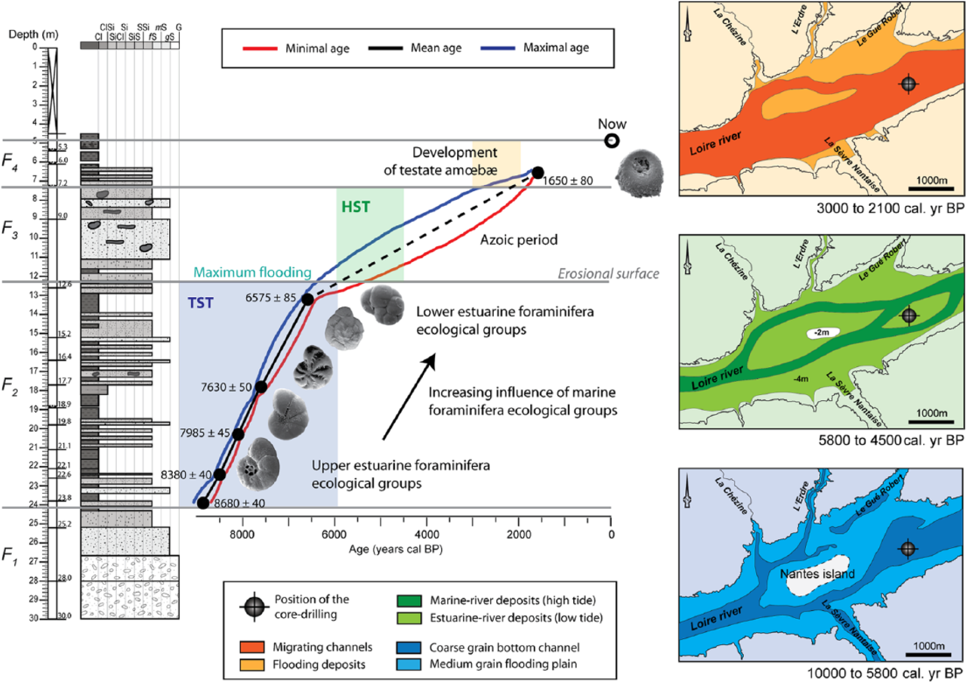
Diagram of the Nantes Island infilling evolution with age–depth model, microfauna evolution, and reconstructed maps of Nantes Island zone (modified after Arthuis and Nauleau, 2008.

The earliest sediment deposits (Section F₁) are constituted of coarse particles associated with illite and chlorite clay minerals. These sediments are probably produced by soil erosion and the reworking of the metamorphized Paleozoic bedrock, triggered by high hydrodynamics. As many Atlantic estuaries, this rocky substrate bedrock corresponds to the Holocene basement described by Proust et al. (2010) close to Saint-Nazaire (50 km downstream). Moreover, the scarcity and the great variability of foraminifera EGs observed during this period testify to the high hydrodynamics and are of a dominant marine influence. These sediments probably correspond to reworked fluvial sediments deposited during the period of low sea level along the Pleistocene glacial stage (Lowstand Systems Tract, LST; Posamentier and Allen, 1999). These earliest deposits (Section F₁) probably correspond to the early Holocene (defined by Walker et al., 2012), prior to 8850 cal. yr BP.

The second section (F₂) extends from 8850 (24.2 m) to 5850 cal. yr BP (12.2 m). The sediment deposits are typical of an estuary, and are composed of an alternation of clay and fine sand layers, with high foraminiferal density and diversity (Figure 5). The clay fraction is enriched in smectite, which could have two origins: an increase of the runoff of the Sèvre Nantaise River; and/or increased marine influence, as continentally derived smectite would easily flocculate with an increase in water salinity. These deposits are characteristic of a tidal regime, with a regular deposit of fine particles in which estuarine foraminifera EGs could develop. Marine fauna EGs also regularly occurred, depending on the speed of the infilling. By the same way Llyod (2000), in an isolated basin in Scotland (UK), observed high diversity from 9100 to 6700 BP. Variations of diversity were, however, less marked than those observed in Loire estuary. The C/N, always of intermediate value during that period, confirm these typical estuarine conditions. This section, deposited during the mid Holocene, is characterized by a TST deposit under a tidal dynamic. This period is marked by the transgression associated with the increase in the available space for the sediment infilling. These observations corroborate the study of Perez-Belmonte (2008) that described an oceanic invasion of the Golfe du Morbihan (65 km from the Loire estuary) that occurred from 9000 to 5000 cal. yr BP during the end of the Flandrian transgression, conducting the establishment of the TST. These observations also corroborate the large consensus after studies of Ters (1986) that defined TST from 11.7 to 6 years BP along the French Atlantic coasts. The TST is controlled by glacio-eustatism (Posamentier and Allen, 1999). The end of the TST is marked by the Maximum Flooding Surface (MFS).

The third section (F₃) is characterized by sandy deposits of continental origin subjected to erosion, which make an incision in the former TST, and corresponds to an HST. Indeed, from 5850 to 2100 cal. yr BP, the sediment clay fraction is composed of high levels of illite. This may be interpreted as reflecting a high erosion regime or intense reworking, due to the decrease in the speed of the sea level rise, which is inferior to the sedimentation rate. This section is almost azoic, which fits with the notion of high hydrodynamics. The migration of the channel implies a lack of the deposit that could occur all along this period, from 11.2 m (5100 cal. yr BP) to 7.5 m (2350 cal. yr BP). This erosive period extends during the mid to late Holocene. By the same way, Perez-Belmonte (2008) in the Golfe du Morbihan observed that after ca. 5000 cal. BP, the established HST is subjected to frequent erosive episodes because of external and internal forcing. During that period, the coastline shifted towards the ocean (Posamentier and Allen, 1999). This shift is associated with a migration of the main sediment depositional zone, located on the shelf, off the estuaries that flow towards the Bay of Biscay (Poirier, 2010; Traini, 2009). This change implied change in the environmental conditions and forced the foraminiferal fauna to migrate or disappear, replaced by testate amoebae. These observations are the same for Lloyd (2000) where diversity is low and fauna is dominated by brackish fauna. Controlling factors could be of (1) climatic origin (recurrence of storms; Chaumillon et al., 2010 and references therein), (2) the reduction of the available space after the transgression that thus limit the conservation of recently deposited sediments (Clavé et al., 2001), and (3) human activity as for example here testified by C/N results (Poirier, 2010).

The last section (F₄) extends from 2100 cal. yr BP (7.2 m depth) to the top of the analysed sediments. The sediments are composed of a succession of clayey and sandy layers. The combination of the development of testate amoebae, the absence of foraminifera, the decrease in illite and increase of smectite and kaolinite proportions support the hypothesis of a continentalization of the environment. The environment is under the strong influence of freshwater. In the small basin described by Lloyd (2000), testate amoebae are occurring from 700 BP. In Loire estuary, testate amoebae are occurring earlier, probably because the study area is far more inland.

The samples labelled RS in Figures 2 and 7 have sediment and faunal characteristics that are similar to the sediment observed in Section F₂. As a consequence, they probably correspond to reworked sediments dredged from the main channel and deposited as embankments.

Conclusion

The main stages of the Holocene Loire Valley evolution in Nantes are as follows:

Up to 8850 cal. yr BP. A high water dynamic period due to an early Holocene transgression, the erosion of the metamorphic substratum, deposits of coarse particles, and rare transported microfaunal specimens. The sediments are structured in an LST.

From 8850 to 5850 cal. yr BP. An estuarine dynamic period with abundant and diverse typical foraminifera species. The sediments show an alternation of clayey/sand deposits. The marine influence is increasing. The sediment deposit is structured in a TST.

From 5850 to 2100 cal. yr BP. A fall in the sea level rise and the available space for sedimentation. There is migration of the channels and intense movement of the sediment. The sediments are structured in an HST. Fauna are rare in this highly dynamic context.

From 2100 cal. yr BP to the present. Continentalization. Testate amoebae are settling in a freshwater environment.

Footnotes

Funding

This present work was financially supported by the European community (Fonds européen de développement régional (FEDER)), the Service Régional de l’Archéologie des Pays de la Loire, the Conseil Régional des Pays de la Loire, the Conseil Général de Loire Atlantique, Nantes city.

References

Alve

Murray

(1999) Marginal marine environments of the Skagerrak and Kattegat: A baseline study of living (stained) benthic foraminiferal ecology. Palaeogeography, Palaeoclimatology, Palaeoecology 146: 171–193.

Armynot du Châtelet

Bout-Roumazeilles

Riboulleau

. (2009) Sediment (grain size and clay mineralogy) and organic matter quality control on living benthic foraminifera. Revue de micropaléontologie 52: 75–84.

Armynot du Châtelet

Debenay

J-P

Degré

. (2005) The use of benthic foraminifera as sea-level indicators? Case study of the Aiguillon cove [Utilisation des foraminifères benthiques comme indicateurs de paléo-niveaux marins? Étude du cas de l’anse de l’Aiguillon]. Comptes Rendus Palevol 4: 209–223.

Armynot du Châtelet

Guillot

Recourt

. (2010) Influence of sediment grain size and mineralogy on testate amoebae test construction. Comptes Rendus Geoscience 342: 710–717.

Armynot du Châtelet

Noiriel

Delaine

(2013) Three-dimensional morphological and mineralogical characterization of testate amebae. Microscopy and Microanalysis 19: 1511–1522.

Arthuis

Nauleau

J-F

(2008) La Loire à Nantes: bilan sédimentaire, conséquences géomorphologiques et archéologiques. Préliminaires à l’étude du paysage. Rapport PCR “Des Ponts-de-Cé à l’Estuaire, interactions Homme/Milieu de la Loire et ses affluents”, Tome II. Nantes: SRA-Inrap GO.

Asioli

Medioli

Patterson

(1996) Thecamoebians as a tool for reconstruction of paleoenvironments in some Italian lakes in the Foothills of the southern Alps (Orta, Varese and Candia). Journal of Foraminiferal Research 26: 248–263.

Bernhard

(1986) Characteristic assemblages and morphologies of benthic foraminifera from anoxic, organic-rich deposits: Jurassic through Holocene. Journal of Foraminiferal Research 16: 207–215.

Beyens

Chardez

(1995) An annotated list of testate amoebae observed in the Arctic between the longitudes 27°E and 168°W. Archiv fur protistenkunde 144: 137–142.

10.

Blaauw

Christen

(2011) Flexible paleoclimate age-depth models using an autoregressive gamma process. Bayesian Analysis 6: 457–474.

11.

Boltovskoy

Wright

(1976) Recent foraminifera. The Hague: W. Junk.

12.

Booth

Jackson

Gray

CED

(2004) Paleoecology and high-resolution paleohydrology of a kettle peatland in upper Michigan. Quaternary Research 61: 1–13.

13.

Bout-Roumazeilles

Combourieu-Nebout

Desprat

. (2013a) Tracking atmospheric and riverine terrigenous supplies variability during the last glacial and the Holocene in central Mediterranean. Climate of the Past 9: 1065–1087.

14.

Bout-Roumazeilles

Cortijo

Labeyrie

. (1999) Clay mineral evidence of nepheloid layer contribution to the Heinrich layers in the Northwest Atlantic. Palaeogeography, Palaeoclimatology, Palaeoecology 146: 211–228.

15.

Bout-Roumazeilles

Riboulleau

Armynot

Châtelet

. (2013b) Clay mineralogy of surface sediments as a tool for deciphering river contributions to the Cariaco Basin (Venezuela). Journal of Geophysical Research – Oceans 118: 750–761.

16.

Brady

(1884) Report on the Foraminifera dredged by H.M.S. Challenger during the years 1873–1876. Scientific results of the voyage of H.M.S. Challenger during the years 1873–1876. Zoology 9: 1–814.

17.

Brindley

Brown

(1980) Crystal Structures of Clay Minerals and Their X-Ray Identification. London: Mineralogical Society.

18.

Cash

Hopkinson

(1905) The British Freshwater Rhizopoda and Heliozoa. London: Printed for the Ray Society.

19.

Charman

(2001) Biostratigraphic and palaeoenvironmental applications of testate amoebae. Quaternary Science Reviews 20: 1753–1764.

20.

Chaumillon

Tessier

Reynaud

(2010) Stratigraphic records and variability of incised valleys and estuaries along French coasts. Bulletin de la Société Géologique de France 181: 75–85.

21.

Ciffroy

Reyss

J-L

Siclet

(2003b) Determination of the residence time of suspended particles in the turbidity maximum of the Loire estuary by 7Be analysis. Estuarine, Coastal and Shelf Science 57: 553–568.

22.

Cimerman

Langer

(1991) Mediterranean Foraminifera. Ljubljana: Slovenska akademija znanosti in umetnosti, 118 pp.

23.

Clarke

(2003) Guide to the Identification of Soil Protozoa – Testate Amoebae. Ambleside: Freshwater Biological Association (Special Publication 12), 40 pp.

24.

Clavé

Massé

Carbonel

. (2001) Holocene coastal changes and infilling of the La Perroche marsh (French Atlantic coast). Oceanologica Acta 24(4): 377–389.

25.

Corliss

Chen

(1988) Morphotype patterns of Norwegian Sea deep-sea benthic foraminifera and ecological implications. Geology 16: 716–719.

26.

Dalrymple

(2006) Incised valleys in time and space: An introduction. In: Dalrymple

Leckie

Tillman

(eds) Incised valleys in time and space. Tulsa, OK: SEPM Special Publication (Society for Sedimentary Geology), pp. 5–12.

27.

Dalrymple

(2010) Tidal depositional systems. In: James

Dalrymple

(eds) Facies Models 4 (GEOtext 6). St John’s: Geological Association of Canada, pp. 201–231.

28.

Delfau

Le Berre

(1981) Définition de zones favorables à la prospection du kaolin dans le massif armoricain. Orléans: BRGM Orléans.

29.

Duleba

Debenay

J-P

(2003) Hydrodynamic circulation in the estuaries of Estaçao Ecologica Jureia-Itatins, Brazil, inferred from foraminifera and thecamoebian assemblages. Journal of Foraminiferal Research 33: 62–93.

30.

Duleba

Debenay

J-P

Beck-Eichler

. (1999) Holocene environmental and water circulation changes: Foraminifer morphogroups evidence in Flamengo Bay (SP, Brazil). Journal of Coastal Research 15: 554–571.

31.

Edwards

Horton

(2000) Reconstructing relative sea-level change using UK salt-marsh foraminifera. Marine Geology 169: 41–56.

32.

Eichler

PPB

Castelao

Pimenta

. (2004) Foraminifera and thecamoebians as indicator of hydrodynamic process in a choked coastal lagoon, Laguna Estuarine System, SC, Brazil. Journal of Coastal Research 39: 1144–1148.

33.

Ellison

(1995) Paleolimnological analysis of Ullswater using testate amoebae. Journal of Paleolimnology 13: 51–63.

34.

Esteoule-Choux

(1967) Contribution à l’étude des argiles du massif armoricain. Argiles des alterations et argiles des bassins sédimentaires tertiaires. Rennes: Université de Rennes.

35.

Etcheber

Taillez

Abril

. (2007) Particulate organic carbon in the estuarine turbidity maxima of the Gironde, Loire and Seine estuaries: Origin and lability. Hydrobiologia 588: 245–259.

36.

Gehrels

Roe

Charman

(2001) Foraminifera, testate amoebae and diatoms as sea-level indicators in UK saltmarshes: A quantitative multiproxy approach. Journal of Quaternary Science 16: 201–220.

37.

Goubert

Neraudeau

Rouchy

. (2001) Foraminiferal record of environmental changes: Messinian of the Los Yesos area (Sorbas Basin, SE Spain). Palaeogeography, Palaeoclimatology, Palaeoecology 175: 61–78.

38.

Haynes

(1981) Foraminifera. New York: John Wiley and Sons, 43 pp.

39.

Hayward

Scott

Grenfell

. (2004) Estimation of tidal elevation and salinity histories of sheltered harbours and estuaries using benthic foraminifera. The Holocene 14: 218–232.

40.

Jalut

(1995) Analyse pollinique de sédiments holocènes de l’étang de Capestang (Hérault). In: Guilaine

(ed.) Temps et espace dans le bassin de l’Aude du Néolithique à l’âge du Fer. Toulouse: Centre d’Anthropologie, pp. 293–303.

41.

Jones

Charnock

(1985) ‘Morphogroups’ of agglutinating foraminifera. Their life positions and feeding habits and potential applicability in (paleo)ecological studies. Revue de Paléobiologie 4: 311–320.

42.

Lee

Anderson

(1991) Biology of foraminifrea. London; San Diego, CA; New York; Boston, MA; Sydney; Tokyo; Toronto: Academic Press.

43.

Lee

Leedale

Bradbury

(2000) An Illustrated Guide to the Protozoa. Lawrence, KS: Allen Press Inc.

44.

Leidy

(1879) Fresh-Water Rhizopods of North America. Washington, DC: Government Printing Office.

45.

Leorri

Gehrels

Horton

. (2010) Distribution of foraminifera in salt marshes along the Atlantic coast of SW Europe: Tools to reconstruct past sea-level variations. Quaternary International 221: 104–115.

46.

Lloyd

(2000) Combined foraminiferal and thecamoebian environmental reconstruction from an isolation basin in NW Scotland: Implications for sea-level studies. Journal of Foraminiferal Research 30: 294–305.

47.

Lopez-Garcia

Lopez-Saez

(2000) Le paysage et la phase épipaléolithique–mésolithique dans les pré-Pyrénées aragonaises et le bassin moyen de l’Èbre à partir de l’analyse palynologique. In: Les derniers chasseurs-cueilleurs d’Europe occidentale (13000–5500 av. J.-C.): Actes du colloque international de Besançon, 23–25 October 1998. Besançon: Presses-Universitaires Franc-Comtoises, pp. 59–69.

48.

Magno

Bergamin

Finoia

. (2012) Correlation between textural characteristics of marine sediments and benthic foraminifera in highly anthropogenically-altered coastal areas. Marine Geology 315–318: 143–161.

49.

Medioli

Scott

(1988) Lacustrine thecamoebians (mainly arcellaceans) as potential tools for palaeolimnological interpretations. Palaeogeography, Palaeoclimatology, Palaeoecology 62: 361–386.

50.

Menier

(2003) Morphologie et remplissage des vallées sud-armoricaines: Apports de la stratigraphie sismique. Lorient: Université de Bretagne Sud, 204 pp.

51.

Meyers

(1994) Preservation of elemental and isotopic source identification of sedimentary organic matter. Chemical Geology 114: 289–302.

52.

Mitchell

EAD

Payne

Lamentowicz

(2008) Potential implications of differential preservation of testate amoeba shells for paleoenvironmental reconstruction in peatlands. Journal of Paleolimnology 40: 603–618.

53.

Montero-Serrano

J-C

Bout-Roumazeilles

Carlson

. (2011) Contrasting rainfall patterns over North America during the Holocene and Last Interglacial as recorded by sediments of the northern Gulf of Mexico. Geophysical Research Letters 38: L14709.

54.

Murray

(1986) Living and dead Holocene foraminifera of Lyme Bay, Southern England. Journal of Foraminiferal Research 16: 347–352.

55.

Murray

(2001) The niche of benthic foraminifera, critical thresholds and proxies. Marine Micropaleontology 41: 1–7.

56.

Murray

(2006) Ecology and Applications of Benthic Foraminifera. Cambridge: Cambridge University Press.

57.

Neville

McCarthy

FMG

MacKinnon

(2010) Seasonal environmental and chemical impact on thecamoebian community composition in an oil sands reclamation wetland in Northern Alberta. Palaeontologia Electronica 13: 13A (14 pp.).

58.

Nguyen-Viet

Bernard

Mitchell

EAD

. (2008) Effect of lead pollution on testate amoebae communities living in Sphagnum fallax: An experimental study. Ecotoxicology and Environmental Safety 69: 130–138.

59.

Ogden

Hedley

(1980) An Atlas of Freshwater Testate Amoebae. Oxford: Oxford University Press.

60.

Ooms

Beyens

Temmerman

(2011) Testate amoebae as estuarine water-level indicators: Modern distribution and the development of a transfer function from a freshwater tidal marsh (Scheldt estuary, Belgium). Journal of Quaternary Science 26: 819–828.

61.

Ottmann

Alix

Limasset

. (1968) Sur ‘le lit ancien’ de la Loire dans son cours inférieur. Bulletin du BRGM 1: 26–56.

62.

Perez-Belmonte

(2008) Caractérisation environnementale, morphosédimentaire et stratigraphique du Golfe du Morbihan pendant l’Holocène terminal: Implications évolutives. Lorient: Université de Bretagne Sud, 219 pp.

63.

Poirier

(2010) Enregistrement couplé par la macrofaune et la microfaune des variations environnementales récentes en Baie de Marennes-Oléron. La Rochelle: Université de la Rochelle, 213 pp.

64.

Posamentier

Allen

(1999) Siliciclastic Sequence Stratigraphy: Concepts and Applications (SEPM Concepts in Sedimentology and Paleontology 7). Tulsa, OK: Society of Paleontologists and Mineralogists, 210 pp.

65.

Proust

Renault

Guennoc

. (2010) Sedimentary architecture of the Loire River drowned valleys of the French Atlantic shelf. Bulletin de la Société Géologique de France 181: 129–149.

66.

Puertas

(1997) Évolution de la végétation depuis le Dryas récent dans la plaine littorale de Montpellier (Hérault, France) à partir de l’analyse pollinique. Dynamique naturelle et anthropisation du milieu. Thèse de Doctorat, Université de Franche-Comté, 337 pp.

67.

R-Development Core Team (2014) R: A Language and Environment for Statistical Computing. Vienna: R Foundation for Statistical Computing. Available at: http://www.R-project.org.

68.

Reimer

Bard

Bayliss

. (2013) IntCal13 and Marine13 radiocarbon age calibration curves 0–50000 years cal BP. Radiocarbon 55:1869–1887.

69.

Richard

(1994) Indices polliniques d’une néolithisation précoce sur le premier plateau du Jura (France). Comptes Rendus de l’Académie des Sciences Paris, série II 318: 993–999.

70.

Roe

Charman

Gehrels

(2002) Fossil testate amoebae in coastal deposits in the UK: Implications for studies of sea-level change. Journal of Quaternary Science 17: 411–429.

71.

Schönfeld

(2002) A new benthic foraminiferal proxy for near-bottom current velocities in the Gulf of Cadiz, northeastern Atlantic Ocean. Deep-Sea Research Part I: Oceanographic Research Papers 49: 1853–1875.

72.

Scott

Medioli

Schafer

(2001) Monitoring in Coastal Environments using Foraminifera and Thecamoebian Indicators. New York: Cambridge University Press.

73.

Sen Gupta

(1999) Chapter 1: Introduction to modern Foraminifera. In: Sen Gupta

(ed.) Modern Foraminifera. Dordrecht: Kluwer Academic Publishers, 371 pp.

74.

Severin

(1983) Test morphology in benthic foraminifera as discriminator of biofacies. Marine Micropaleontology 8: 65–76.

75.

Sorrel

Tessier

Demory

. (2010) Sedimentary archives of the French Atlantic coast (inner Bay of Vilaine, south Brittany): Depositional history and late Holocene climatic and environmental signals. Continental Shelf Research 30: 1250–1266.

76.

Swindles

Roe

(2007) Examining the dissolution characteristics of testate amoebae (Protozoa: Rhizopoda) in low pH conditions: Implications for peatland palaeoclimate studies. Palaeogeography, Palaeoclimatology, Palaeoecology 252: 486–496.

77.

Ters

(1986) Variations in Holocene sea level on the French Atlantic coast and their climatic significance. In: Rampino

Sanders

Newman

. (eds) Climate: History, Periodicity and Predictability. New York: Van Nostrand Reinhold, pp. 204–237.

78.

Ters

Planchais

Azema

(1968) L’évolution de la basse vallée de la Loire, à l’aval de Nantes, à la fin du Wurm et pendant la transgression flandrienne. Bulletin de l’Association française pour l’étude du Quaternaire 5: 217–246.

79.

Thinon

Menier

Guennoc

. (2008) Carte géologique à 1/250 000 de la marge continentale, feuille Lorient (ed Proust

Guennoc

). Orléans: BRGM, CNRS.

80.

Traini

(2009) L’estuaire de la Vilaine: Évolution naturelle et anthropisation (Morbihan, France). Thèse de Doctorat, Université de Bretagne Sud.

81.

Traini

Menier

Proust

. (2013) Transgressive systems tract of a ria-type estuary: The late Holocene Vilaine River drowned valley (France). Marine Geology 337: 140–155.

82.

Trentesaux

Recourt

Bout-Roumazeilles

. (2001) Carbonate grain-size distribution in hemipelagic sediments from a laser particle sizer. Journal of Sedimentary Research 71: 858–862.

83.

Van Hengstum

Reinhardt

Beddows

. (2008) Thecamoebians (testate amoebae) and foraminifera from three anchialine cenotes in Mexico: Low salinity (1.5–4.5 psu) faunal transitions. Journal of Foraminiferal Research 38: 305–317.

84.

Vazquez Riveiros

Babalola

Boudreau

REA

. (2007) Modern distribution of salt marsh foraminifera and thecamoebians in the Seymour-Belize Inlet Complex, British Columbia, Canada. Marine Geology 242: 39–63.

85.

Visset

Cyprien

Carcaud

. (2002) The onset of diversified agriculture at the end of the Mesolithic period in the Val de Loire (Armorican Loire, France). Comptes Rendus Pale 11: 51–58.

86.

Visset

Hauray

Charrieau

. (2001) Paléo-environnement urbain: Histoire du comblement des vallées de la métro- pole nantaise, du Tardiglaciaire à la fin de l’Holocène. Annales de Bretagne et des Pays de l’Ouest 108(1): 147–165.

87.

Walker

MJC

Berkelhammer

Björck

. (2012) Formal subdivision of the Holocene Series/Epoch: A Discussion Paper by the Working Group of INTIMATE (Integration of ice-core, marine and terrestrial records) and the Subcommission on Quaternary Stratigraphy (International Commission on Stratigraphy). Journal of Quaternary Science 27(7): 649–659.

88.

Wall

AAJ

Gilbert

Magny

. (2010) Testate amoeba analysis of lake sediments: Impact of filter size and total count on estimates of density, species richness and assemblage structure. Journal of Paleolimnology 43: 689–704.

89.

Zaitlin

Dalrymple

Boyd

(1994) The stratigraphic organization of incised-valley systems associated with sea-level change. In: Dalrymple

Boyd

Zaitlin

(eds) Incised-Valley Systems: Origin and Sedimentary Sequences. Tulsa: SEPM (Special Publication 51), pp. 45–60.

Supplementary Material

Please find the following supplemental material available below.

For Open Access articles published under a Creative Commons License, all supplemental material carries the same license as the article it is associated with.

For non-Open Access articles published, all supplemental material carries a non-exclusive license, and permission requests for re-use of supplemental material or any part of supplemental material shall be sent directly to the copyright owner as specified in the copyright notice associated with the article.

0.00 MB

0.16 MB

0.01 MB