



Abstract
In this article, we present an asset management-based methodology for the integration and deployment of guardrail sensors into an existing Intelligent Transportation System (ITS). The methodology employs a three phase approach that incorporates data modeling, spatial analysis using Geographic Information Systems (GIS), and cost optimization to provide enhanced decision support when integrating guardrail sensing capabilities into an existing ITS. The utility of the proposed methodology is illustrated through an example integration of a guardrail sensor network in high collision segment of roadways in a metropolitan area of Montgomery, Ohio. The results demonstrate that the methodology provides an effective means for planning new sensor deployments by providing a structured approach to modeling the existing ITS, identifying optimal sensor placement, and analyzing cost and performance tradeoffs to yield the optimal solution for a given set of requirements.
Introduction
United States (U.S.) roadways are deteriorating as a result of increased age and use (Schofer et al., 2010). Based upon this recognition, the U.S. Department of Transportation (DOT) and Transportation Research Board (TRB) facilitated a meeting of infrastructure stakeholders to consider problems, needs, achievements and to define the direction for research to manage and preserve the nation’s surface transportation infrastructure. The group identified three areas needing further research: The development of infrastructure condition and performance monitoring, the development of methods for the rapid testing of materials, and the investigation of new transportation infrastructure designs. This article addresses the integration of new sensors used for infrastructure condition and performance monitoring into an existing Intelligent Transportation System (ITS). Specifically, this article shows the data integration and systems modeling used to incorporate impact sensors into guardrail systems for the purpose of maintenance notification and possibly emergency system response.
An ITS can be used to both monitor the state of the infrastructure in real time and to collect aggregate statistics over time of parameters related to the infrastructure life cycle (Schofer et al., 2010). The ITS concept was developed to leverage modern communication and computing technologies to improve the overall efficiency of transportation systems and infrastructure (Tarko & Rouphail, 1997). The ITS concept is not new as it has been in existence for decades (Kraft, 1999). Modern ITSs collect information about environmental conditions, the volume and speed of traffic, and communicate information back to motorists via message boards. The need for ITS results from a shift from the construction of new highway infrastructure to managing and maintaining the current highway infrastructure as the construction of roads is now considered to be complete (Wootton, 1995). As the Federal Highway Administration (FHWA) stated, the United States Interstate Highway System neared completion in the early 1990s after 40 years of construction (Cambridge Systematics, 1999). Although some minor construction is still ongoing the majority of the effort has shifted from construction to the maintenance, management, and reconstruction of the nation’s roadways. Making this shift is necessary as those highways that were constructed are now suffering from increased usage, environmental issues, and age (Cambridge Systematics, 1999).
Over the years, a number of improved sensing and data collection in the transportation infrastructure have been developed. While work continues on the development of new sensing capabilities for use in the transportation infrastructure, little discussion has focused upon an Asset Management (AM) view of planning and deploying new sensors. AM can be described as “a foundation from which to monitor the transportation system and optimize the preservation, upgrading, and timely replacement of highway assets through cost effective management, programming, and resource allocation decisions” (FHWA, 1999). AM is a basis to manage the transportation assets currently in use across the United States. The hasty implementation of new technologies without the proper life cycle planning can result in suboptimal deployment designs, poor performance, and excessive costs. What is needed is a structured methodology that can be applied for the planning and deployment of any new sensor into an existing ITS. The methodology should support an asset management-based decision making process for implementing new transportation assets. The methodology should specifically address issues including how to integrate new sensors into an existing ITS, how to select the optimal placement of sensors based upon geospatial information and statistics, how to select the optimal set of hardware equipment to link a network of sensors to the ITS at minimum cost, and how to evaluate tradeoffs in system design over a variety of time horizons.
In this article, we present a generalized methodology that can be used for planning the deployment of any type of sensors into an existing ITS. The methodology leverages data modeling, spatial analysis in Geographic Information Systems (GIS), and cost optimization to provide enhanced decision support when planning the deployment of new sensing capabilities within an existing ITS. The remainder of this article is structured as follows: in the second section, we propose a three phase methodology for integrating new sensors into an ITS; in the third section, we apply the methodology to the integration of a guardrail sensor network located within a major metropolitan area in Montgomery county, Ohio into the Ohio Department of Transportation (ODOT) ITS and discuss the process in detail; and in the final section, we present our conclusions and discuss future research directions.
An Asset Management-Based Methodology for Integrating Sensors Into an Existing ITS
In this section, we present a three phase methodology for the deployment of a new sensor within an existing ITS. Each of the three phases is executed sequentially, and the result is a plan for the optimal deployment of the sensor network.
Phase I—Documenting the Existing Intelligent Transportation System (ITS)
The purpose of the first phase is to develop models to describe and document the ITS architecture which are necessary to understand when integrating a new sensor. Before modeling can begin it is necessary to understand what the existing system consists of including sensors, collection boxes, reach back systems and databases. In modeling the existing system, the requirements for a new component(s) become clear. Understanding all the system components allows the person doing the modeling to understand the direction of flow of data, how much data are created and the type of data used. It also allows for an understanding of the organization of the data within the database(s).
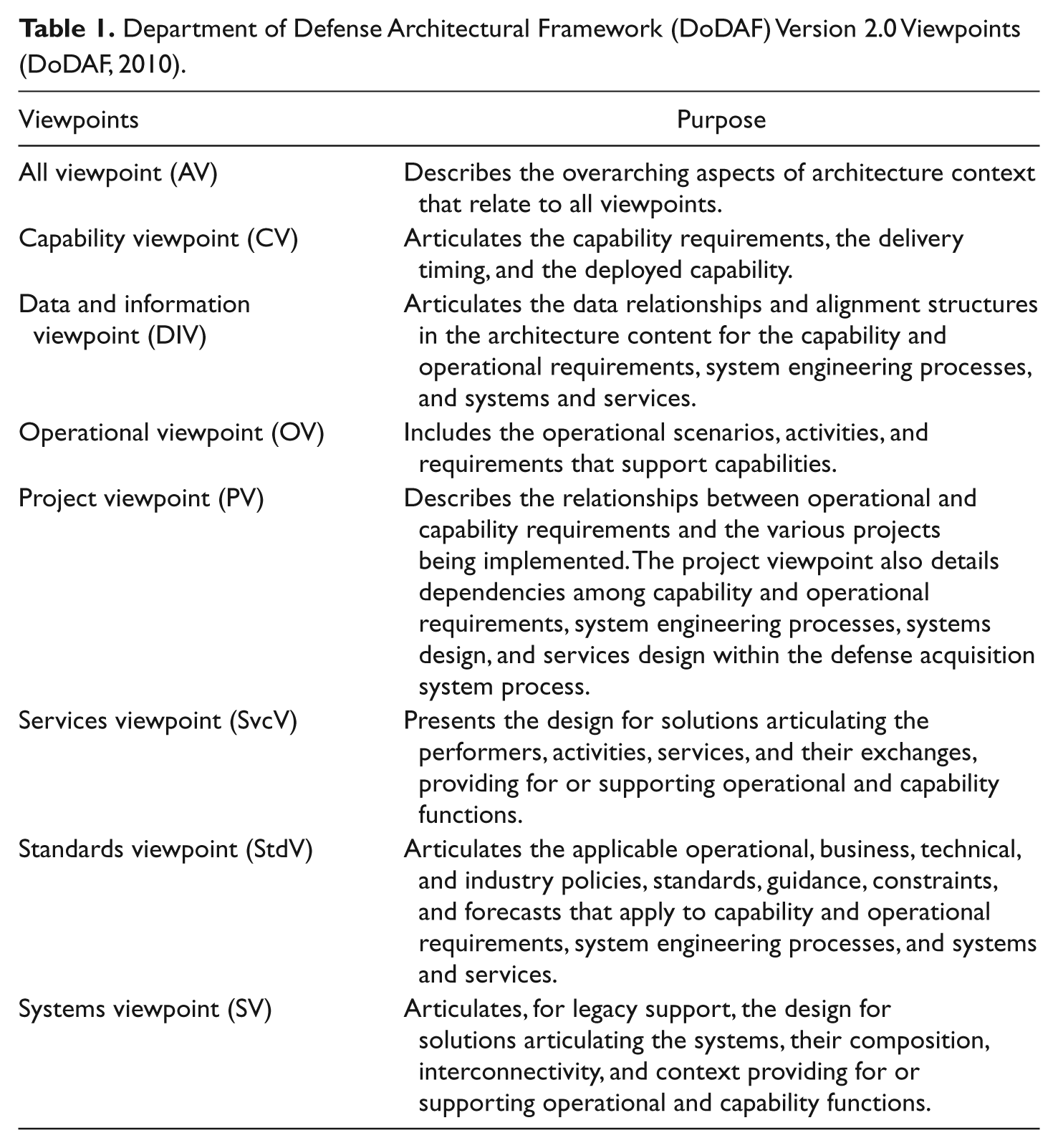
The format for documenting the requirements can come from several different approaches. The format is largely impacted by the type of analysis required and the level of information available to fully understand the complexity of the system being modeled (Longley, Goodchild, Maguire, & Rhind, 2011; Sitzabee, Rasdorf, Hummer, & Devine, 2009). Longley et al. (2011) recommends performing the modeling, from a GIS standpoint, using four levels ranging from reality, which is the understanding of system and major components it is comprised of, to the physical model which is the portrayal of the actual computer implementation. Another approach from the systems engineering perspective is to describe the systems architecture using a series of products which describe the system from multiple viewpoints. Systems architecture is an essential tool in systems engineering because it provides a shared representation of the system from multiple perspectives that can be used by multiple stakeholders to assure consistency and clarity about the composition of the system. For example, the Department of Defense Architecture Framework (DoDAF) version 2.02 defines a set of products, categorized into eight different views that act as mechanisms for visualizing, understanding, and assimilating the broad scope and complexities of the system as shown in Table 1 (DoDAF, 2010). Each view has multiple products to describe the system in terms of the given viewpoint. It is important to note that only a subset of the full DoDAF views, those products that are relevant to system understanding, are typically created to document the system development.
Department of Defense Architectural Framework (DoDAF) Version 2.0 Viewpoints (DoDAF, 2010).
The importance of performing data modeling can be summed up in the following statement; “In many highway agencies separate data management systems are often incompatible and data integration among these systems becomes impractical or expensive” (Gharaibeh, Darter, & Uzarksi, 1999; Sitzabee et al., 2009). An accurate understanding of existing systems is critical to integrate additional components and avoid issues in the future.
Phase II—Geospatial Analysis using a Geographic Information Systems (GIS)
The purpose of the second phase is to exploit spatial analysis using a GIS model to determine the best locations to place the sensors. GIS provides people with the information about where events have occurred (Longley et al., 2011). Knowing where events occur allows for better decisions to be made in regards to the location selection for new transportation infrastructure assets. Additionally, data about these events can also be embedded giving them context and in turn a deeper understanding of the events is gained (Longley et al., 2011). Previous research has already established that a GIS is a powerful system that can integrate various data sources and spatially connect the data to create information about a system that would otherwise be unapparent (Flintsch, Dymond, & Collura, 2004; Sitzabee et al., 2009). The use of GIS allows for sensor locations to be selected based on events particular to the purpose of that sensor. For example, if traffic volume sensors are needed, GIS can be used to identify locations of high traffic. Utilizing GIS can save money by providing accurate locations for sensor placement. Furthermore, location centered asset management allows for a holistic view of the assets in terms of overlapping systems. A sensor that would be placed in a particular system and tracked in a GIS would show other users where the sensor is intended to go. For example, if a temperature sensor was placed in the pavement an asset manager would then have the available data to determine when that pavement is expected to be replaced or overlaid with new pavement. This allows for the asset manager to make the appropriate decisions regarding cost verse benefit of installing the sensor. Another example would is to use GIS accident data to determine the best location for a real-time video camera installation for the purpose of highway monitoring.
The need for GIS comes from the need to solve practical transportation issues (Longley et al., 2011). An example of the use of GIS is the New York State DOT. The New York DOT uses GIS to integrate both pavement and bridge management project information. Symbols on a map representing bridge or pavement projects can be selected to open a window displaying detailed project information (FHWA, 1999). The information allows for the quick reference of projects to understand them spatially on a map as well as find the status of specific projects. GIS allows for the spatial representation of information and for that information to be analyzed (ESRI, 2011). In terms of new transportation assets, information can be analyzed spatially on a map to choose optimal locations for the new asset. The use of spatial analysis tools allows for a variety of analysis to be conducted such as transportation corridors and high incidents of vehicle accidents.
Phase III—Life Cycle Planning and Cost Optimization
The purpose of the third phase is to use cost optimization techniques to identify the minimum cost solution that satisfies the sensor deployment requirements. Information from all phases is used providing the insight necessary to determine the Total Cost of Ownership (TCO). The TCO is a financial estimate used by decision makers to determine direct and indirect costs over the life cycle of a system. While there are many factors which influence the TCO for the deployment of a sensor network system, in this article we focus only on the sensor network itself and not upon the ancillary items required for any installation.
It’s critical to understand that in order to have real-time sensing a reach back network must be in place. Taking this into consideration in determining cost as accurately as possible a model sensor system should be built including the sensor and any reach back equipment necessary. The model can be physical or notional, but by detailing the components of the system using the information garnered from Phases I and II a more realistic cost can be developed for the sensor system. Phase I and II provide the requirements for the hardware necessary for the proposed sensor and optimal locations of network nodes. The hardware requirements provide an understanding of what specifically can be used for components and their respective costs. The network node locations provide the potential size of the system and the reach back that would be required. These two portions combine with the life cycle factors such as length of life of the system and present worth to provide an optimal cost. Present worth determines economic effectiveness and provides a conversion for the system cost each year of its life cycle into present dollars (Canada, Sullivan, Kulonda, & White, 2005).
Life cycle cost analysis (LCCA) provides DOTs a responsible decision making tool and allows for proper asset management. Effective asset management means the management of highway assets and integration of new assets requires economic responsibility and sound investment strategies (FHWA, 1999). In estimating life cycle costs, DOTs and the FHWA can forecast budget requirements and determine the feasibility of a new asset more accurately. LCCA is widely accepted as a useful project evaluation tool and estimates the users cost over the life of a project or system (FHWA, 1999).
LCCA represents an optimization tool that focuses on a critical aspect of AM. Total cost of ownership and the overall economic feasibility of employing new infrastructure assets can be determined with LCCA. Other optimization tools utilized in this research include GIS and data modeling. Each tool hones in on specific attributes of the sensor that must be known in order to integrate it responsibly into an existing ITS network.
Example Application of the Method
In this section, we demonstrate the value of the proposed methodology through the planning required for the deployment of a guardrail sensor network into the ODOT ITS.
Motivation for a Guardrail Sensor Network
Research in the area of the active sensing of guardrail condition is limited. The importance of improving on guardrails was concluded from a study by Michie and Bronstad (1994). The two researchers determined that 6% of guardrail impacts result in injury or fatality and 90% of the total vehicle impacts are unreported entirely (Michie & Bronstad, 1994). Not much is known about this 90%, but most likely some of these result in injuries as well. Furthermore, Michie and Bronstad’s study shows that of the 6% of accidents resulting in injuries or fatalities, many involve guardrails that are out of date, incorrectly constructed, inadequately maintained, or involve accidents that are outside the design range of modern guardrail systems (Michie & Bronstad, 1994). The ability to sense and record guardrail impacts can yield multiple benefits including real-time notification of impacts, reduced emergency service notification times, and reduced resources required for manual damage inspection. Examples of this research include sensor development in similar areas, such as impact detection. Flanigan, Blatt, Russell, Batta, & Kunik (2010) discuss emergency response technology and integrated active transportation systems (IATS). They cite research being performed by the U.S. DOT to create a future transportation infrastructure that improves safety, congestion, energy and environment as well as the infrastructures productivity. One of the most promising technologies the authors studied and that is already in use today was the Advanced Automated Crash Notification Systems (AACN), which use in-vehicle sensors (accelerometers) to sense crash occurrence and characterize the crash severity. The vehicle senses the crash and places a cell phone call to a private telematics service provider (Flanigan et al., 2010).
An alternate strategy is to sense collisions on the guardrail itself. A group of researchers in China investigated guardrail sensing with a monitoring system specifically for vehicle impacts with guardrails (Jiao, Wang, & Zhao, 2008). Their research was motivated by the fact that in China, 55% of all the traffic accidents are on the expressway and 30% of those involve vehicle impacts with guardrails. In terms of fatal traffic accidents, one-third each year are due to vehicle impacts with guardrails. As discussed earlier, approximately 90% of guardrail impacts in the United States are unreported (Michie & Bronstad, 1994). As a consequence, the need for real-time guardrail sensing has never been more important. Jiao et al. (2008) designed and built a wireless sensor network to specifically monitor vibrations within a guardrail during a vehicle impact. The network is comprised of a series of three-axis accelerometers connected to a still image capturing unit via a short distance communication device and a remote control center. Once a vehicle has impacted the guardrail, vibrations are carried to the sensor which then triggers the camera to capture images of what has occurred. While Jiao et al. (2008) concluded with the determination that a guardrail sensor network is both feasible and practical; they did not address the planning required for the deployment of a guardrail sensor network (e.g., deploying guardrail sensors on multiple guardrails in a given geographic area). In this example, we demonstrate how our methodology provides value in the planning required for the deployment of a guardrail sensor network in Montgomery County, Ohio that accounts for the integration with existing infrastructure, selection of which guardrails to be sensed, and the total costs involved with deployment over the life cycle of the system. Note that we focus our analysis on the planning rather than the specific technologies used to construct the guardrail sensor network. This is intentional as the proposed planning methodology is not tied to any specific technology, but instead relies on parameters of the underlying technology as variables (e.g., cost, range, battery life) needed to perform the analysis.
Phase I—Documenting the Existing ODOT Intelligent Transportation System (ITS)
The ODOT ITS is comprised of over 600 nodes and covers a geographical area of over 44,000 square miles, 4,000 square miles of which is contained in urban areas. Sensor information is communicated back from remote locations via Internet Protocol (IP) over existing local area networks or via cellular telephone. Each node has a distinct IP address and provides an aggregation point for multiple sensors within the immediate geographic area of the node. Each node has a small embedded microcontroller with auxiliary data ports which can talk multiple communication protocols (e.g., Ethernet, RS-232, RS-422). This allows a cluster of sensors, each talking a separate protocol, to be queried and the results aggregated into an IP message that is sent back ODOT’s central office located in Columbus, Ohio. Existing sensors within the ODOT ITS include video traffic cameras, road temperature sensors, traffic speed sensors, humidity sensors, railway warning systems, roadway weather systems as well as many others.
In our analysis, we make use of DoDAF products discussed previously to document the ODOT ITS. For brevity, only the two views most relevant to the article are shown as the remaining views are addressed in other research. Figure 1 shows the Systems Viewpoint (SV) -1 view “Systems/Services Interface Description” for the existing ODOT ITS. The SV-1 depicts the systems that make up the ODOT network. While there are many remote nodes in the ODOT ITS, only one prototypical node is shown for clarity. A remote node contains a sensor cluster (e.g., one or more sensors) connected to the control box. The clusters vary and there are a number of configurations that comprise the different sensor combinations across the state; however, each cluster follows the same overall system structure. The distance between each sensor and control box is limited based upon specific data communications interface. For example, a cable carrying RS-232 operating at 9,600 bits per second is limited to 500 feet (Bies, 2010). As a result, sensors must me located within these distance limits. The control box aggregates sensor data into IP packets and then communicates these back to the ODOT Control Node via cellular telephone, radio frequency, or hardwire internet connections. Currently, all remote nodes are powered by dedicated power line run from nearby utilities. ODOT also purchases services from Speed Info which owns their speed sensors and communication reach back capabilities as shown at the bottom of Figure 1.

ODOT SV-1 systems/services interface description.
In order to integrate guardrail sensors into the ODOT ITS, the collected sensor data must be transmitted back to the ODOT Control Node for processing. From SV-1 view, we recognize that using the existing architecture would mean that only a limited number of guardrails, those in close proximity to the Remote Node, could be equipped with sensors to provide active guardrail sensing. For this reason, we consider a collection of guardrails, each equipped with a guardrail sensor control node located at the center of each guardrail that consists of one or more sensors, a microcontroller, a wireless radio, and a battery that are connected together to form a single guardrail sensor network. Each guardrail continuously monitors its sensors and communicates sensor data back on a periodic basis to its nearest neighbor, which in turn passes it to its nearest neighbor, until it arrives at the guardrail designated as the communication reach back node to the ODOT Control Node. The communication reach back can be accomplished by a guardrail that is collocated with an existing Remote Node or, in remote areas lacking power, by a special battery powered cellular telephone.
Figure 2 shows the Data and Information Viewpoint (DIV) -1 view “Systems/Services Interface Description” for the existing ODOT ITS. The DIV-2 is the logical model displaying the data view of the ODOT ITS network. The flow of information is represented in this view as are the measurements and information being collected by individual sensors. The ODOT server queries the sensors and each sensor provides the ODOT server with data on their respective measurements. The Speed Info sensor is a separate system and communicates directly with the ODOT server. The data, once at the ODOT server is then channeled into the individual database tables for each sensor collecting all the information listed on the sensor in addition to the time and location (of the sensor) that the data was collected. This model demonstrates that both being queried and providing data to the database are necessary functions of an ODOT sensor.
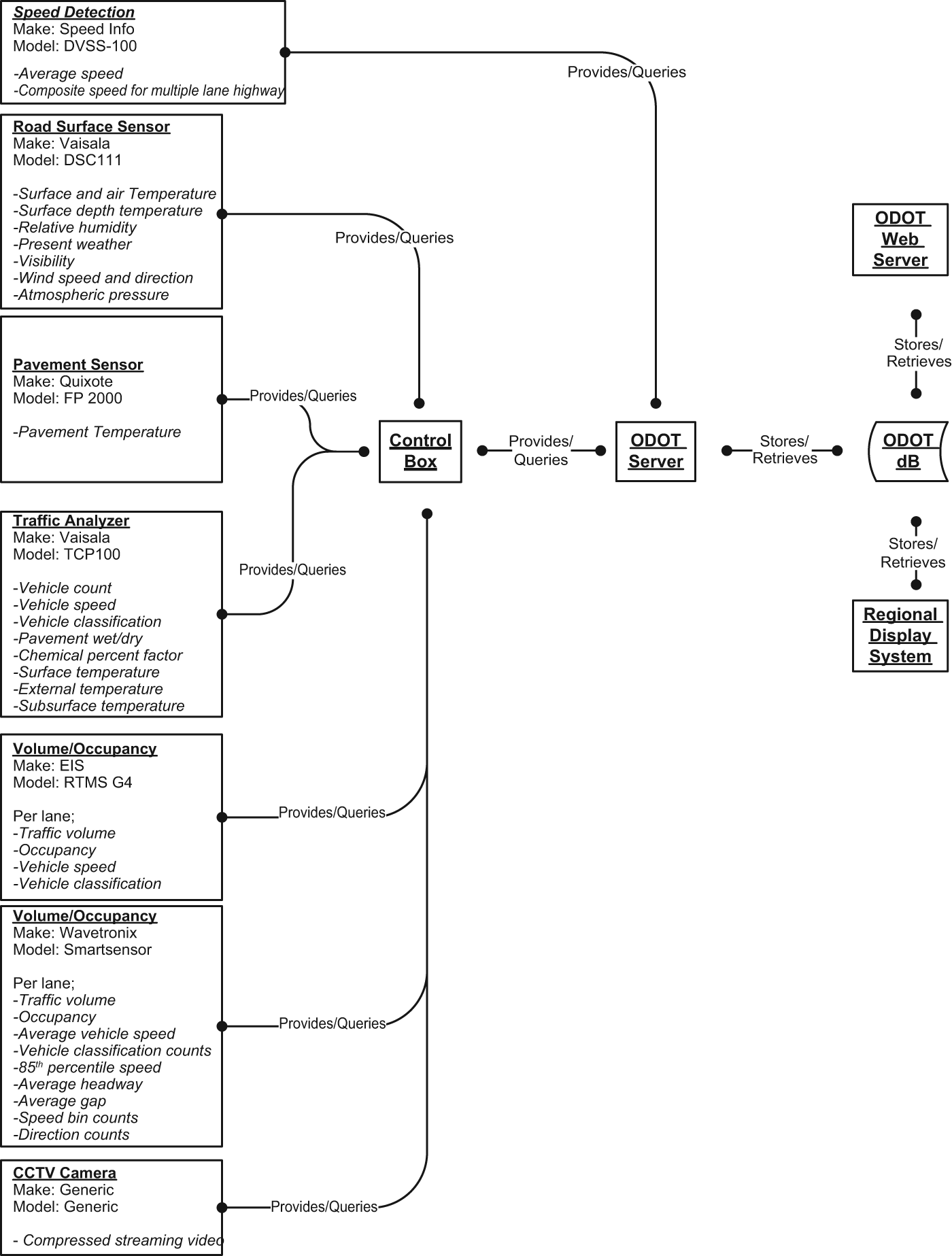
ODOT DIV-2 “Logical Data Model”.
The DIV-2 view reveals that the ODOT ITS was built using standard relational database technologies. As such, any new sensor data can easily be integrated into the database once the sensor data is transported back to the ODOT Control Node via an existing Remote Node or via a new direct Cellular Telephone connection. Based upon this analysis, the addition of a guardrail sensor network will be relatively inexpensive to implement in terms of the hardware and software required at the ODOT Control Node. As we will see, the cost of a guardrail sensor network will be dominated by the costs associated with the deployment, operation, and maintenance of the guardrail sensor network.
In summary, the two DoDAF system architectural views presented provide a detailed understanding of the system as it exists and how difficult it will be to integrate guardrail sensors into the ODOT ITS.
Phase II—Geospatial Analysis for Guardrail Sensing using Geographic Information Systems (GIS)
A GIS density analysis was performed on state owned roads located within Montgomery County, Ohio to determine the optimum locations for guardrail sensors. The major state owned roads include interstates I-675, I-70 and I-75 as well as state routes US 35 and US 40. Narrowing it to those roads specifically, a map was built of these major roadways across Montgomery County (Saylor & Comer, 2011). Crash statistics garnered from the Ohio Department of Public Safety site were loaded into the GIS and used to determine which location along the major roads to focus on (ODOPS, 2011). A density analysis was conducted to determine the optimum location of the guardrail sensors in relation to the existing infrastructure.
Performing the Density Analysis within GIS identifies several areas of high significance based on the number of accidents in those areas. One of the areas of highest density is a longitudinal section outside of any traffic camera locations (second of the two highest incident locations within Montgomery County). Regardless of the absence of traffic camera’s, it’s an area of importance in terms of major accident locations and includes two major roads, I-70 and US 40. It is for that reason that this area was selected for placement of guardrail sensors. As identified in Phase I, ideally one of the guardrails contained in the guardrail sensor network would be colocated with an ODOT Remote Node to provide a communications pathway back to the ODOT Control Node. However, in this case the geographic area selected for guardrail sensing does not contain an existing ODOT Remote Node. For this reason, the guardrail sensor network will have to make use of a battery operated cellular telephone at one of the guardrails in the network to provide the required communications reachback to the ODOT Control Node. Since all of the guardrails are equipped with batteries, it is vital to consider the power consumption of the sensor network and the operational and maintanance costs associated with the use of batteries for power. In this example, 30 guardrails were selected along I-70 and US 40 located in Montgomery county, Ohio.
A preliminary site survey of the location must be conducted to identify potential power and communication utilities, unusual geographic concerns, and any potential obstructions that would affect the range or difficulty in establishing communications links between guardrails. A failure to complete this step can have catastrophic consequences on the success of the project.
Phase III—Minimizing the Total Cost of Ownership of the Guardrail Sensor Network
When selecting among a large number of possible solutions for a given problem, it is essential to exploit optimization tools which select optimal, or near optimal, solutions based upon the problem formulation. In the context of this example, the locations of the 30 guardrails are fixed, but the selection of the hardware and associated costs over the lifecycle of the system must be considered. This requires the formulation of a cost optimization model to determine the optimum mix of hardware to meet the performance requirements while minimizing the TCO over the life cycle of the system. This phase has been broken into three components: (a) Determining the minimum distance required to connect all of the guardrails in the guardrail sensor network, (b) determining the number of sensors placed on each guardrail and their cost, and (c) selecting the communication media for each of the links between the guardrails that meets the performance requirements while minimizing the TCO.
Identification of Minimum Distance Between Guardrail Midpoints
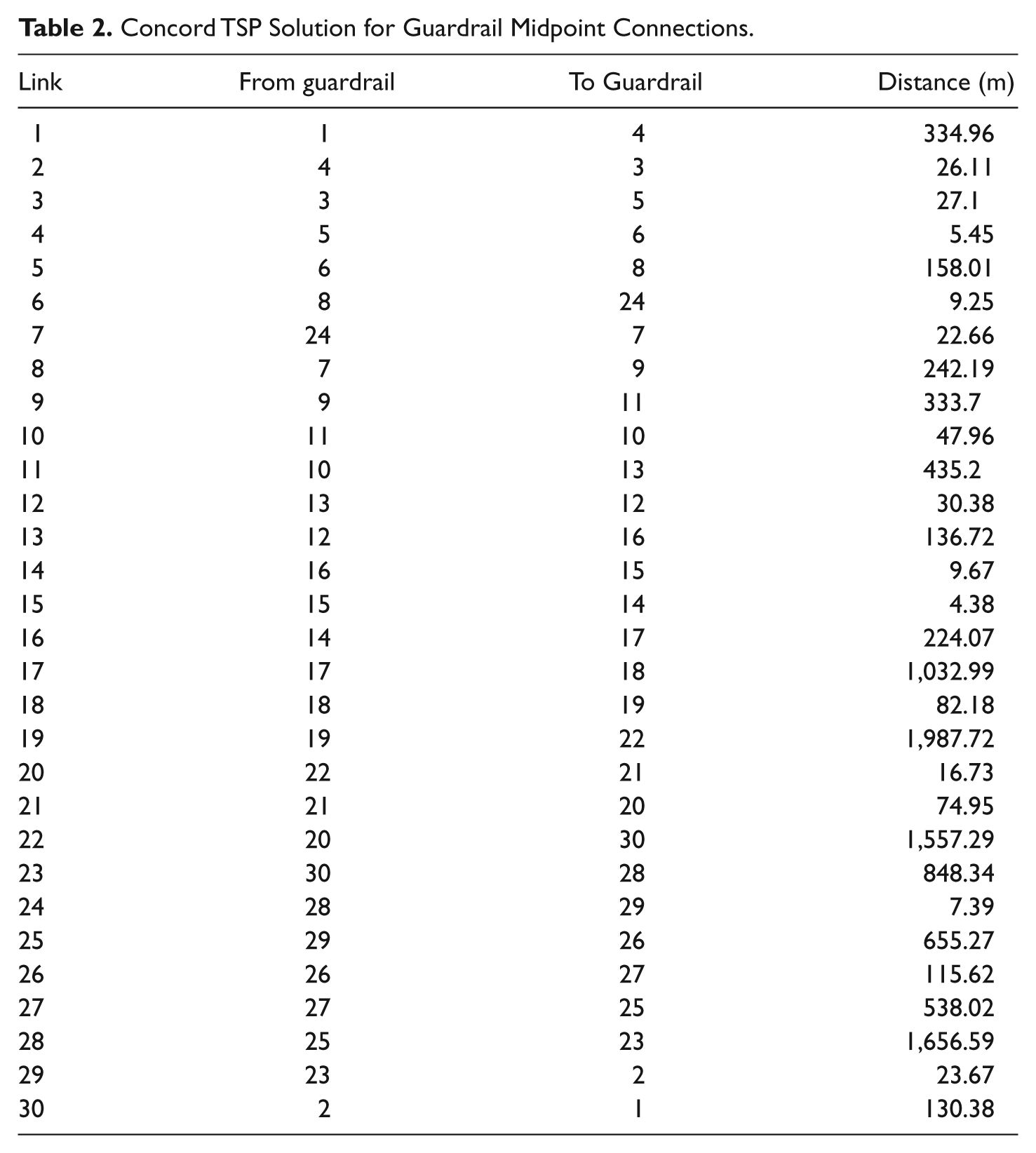
To accomplish the first component, we used the guardrail midpoint coordinates and formulated a Traveling Salesman Problem (TSP) to identify the minimum distance required to interconnect all 30 guardrails (Cook, 2011). The solution to the TSP identifies the 30 minimum distance links necessary to connect all the 30 guardrail midpoints in a closed loop given the constraint that each guardrail midpoint is only visited one time. Since it is not necessary to have a closed loop, we identify and eliminate the maximum length link which still assures all of the remaining guardrails are connected. We formulate the problem in Traveling Salesman Problem Library (TSPLIB) format and used the Concorde software package for solving the TSP and some related network optimization problems (Cook, 2011; Groer, 2008). Collectively, the guardrail nodes form a network that will be connected together using the most cost effective combination of wired and wireless communications media. The Concord optimization required less than 5 sec to complete on an Intel-based PC running Windows 7 operating system with a 3 GHz dual core processor with 4GB RAM and a 500MB disk. The solution for the TSP formulated in the example is shown in Table 2. Note that link 19, which connects guardrails 19 and 22, has the maximum length of 1,987.72 meters. Based upon this analysis, we eliminate this link leaving the remaining 29 links necessary to form the guardrails sensor network. The sum of the remaining link distances is 8,787.23 meters.
Concord TSP Solution for Guardrail Midpoint Connections.
Within each guardrail, one or more sensors (based upon the length of the guardrail) collect data and following an impact sends it to the guardrail node located at the midpoint of the guardrail. The sensor data is than transmitted to its nearest neighbor in a daisy chain manner until it reaches a guardrail that has a communications reach back capability to the ODOT Control Node.
Composition of a Guardrail Sensor Node
The life spans of each sensor were evaluated over a 30 year period and the total cost of each, over the 30 year period, are then converted into a present worth. The discount rate for determining the present worth of each option from the Office of Management and Budget (OMB) is 2.3% for a 30 year period, which is the real interest rate as opposed to the nominal interest rate (OMB, 2011). Using this discount rate, all four costs for the lifetime of each communication type can be evenly evaluated for a 30 year period. The output from this phase is the quantity of each communication type that will be used across all 29 connections and thus the total cost of a sensor cluster over their lifespan. Again, the reason for this phase of the methodology is to determine the optimum blend of performance considering the cost of the individual guardrail sensors and the power source utilized.
Determining the Number of Sensors per Guardrail and Cost
The costs for each guardrail sensor node are determined by specifying the main components including one or more accelerometer sensors, a microcontroller, the communications transceiver (wired or radio), and a battery. The selection of the communications transceiver is addressed in the next section. The number of sensors placed on each guardrail is a function of the length of the guardrail and the maximum sensing distance, MaxRange, for the sensors used to detect collision. The number of sensors required per guardrail is shown below in Equation 1:
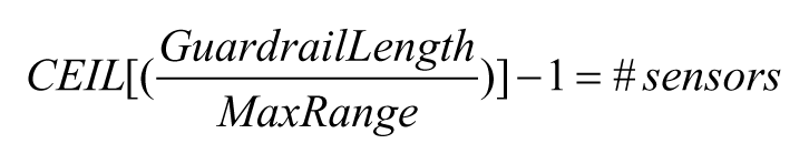
Equation 2 is used to determine the distance between the sensors along the guardrail:

The endpoint coordinates are used to determine the overall length of the guardrails. The length of the guardrails determines the number of sensors required per guardrail and thus allows for the determination in the cost for sensing element for each guardrail. In this example, we assume that each sensor has a maximum vibration sensing range, MaxRange, equal to 50m. In this example, the cost for each sensor contained within a guardrail is assumed to be a fixed US$54 and accounts for the connection back to the microcontroller guardrail sensor node. Each guardrail incurs a fixed cost of US$29 to account for the required microcontroller. This information, together with Equations 1 and 2, yields Table 3, which shows the required number of sensors per guardrail and the cost for sensing in each guardrail.
Number of Sensors per Guardrail and Cost.

Communications Media Selection
The next step involves selecting the minimum cost communications media that satisfies the range requirements at the minimum cost. A Microsoft Excel spreadsheet was used to identify the minimum cost communications media needed to satisfy each of the required 29 guardrail network links. The four communication types include a hardwire cable connection, low power wireless radio, medium power wireless radio and high power wireless radio. Each communication type has a total cost and an effective range. The cost portion of this phase is developed for each communication type separately based on the range of each sensor type, its power source, and its life span. If none of the guardrails is collocated with a Remote Node to provide communications back to the Control Node, a cellular modem must be added to the system components. Each of the guardrail sensor nodes consume a variable amount of power based upon the guardrail size (e.g., the number of sensors is a function of the guardrail length), the maximum distance to the next guardrail in the network, if it contains the cellular modem, and the communications protocols used. It is assumed in this article that the communications protocols have already been optimized to reduce power consumption to extend battery life. If two or more communication types met that range requirement than the least costly type was selected. Table 4 shows the types, costs with installation, and ranges for each type of communication media. It is important to note that the battery size, and hence cost, required for each of the possible communication media accounts not only for communication power consumption but also for the sensing power consumption of each guardrail. This is reasonable because the power consumption for a guardrail sensing nodes is dominated by the communications media, with the sensing power consumption being a relatively fixed amount across all guardrails.
Communication Media Types With Costs and Ranges.
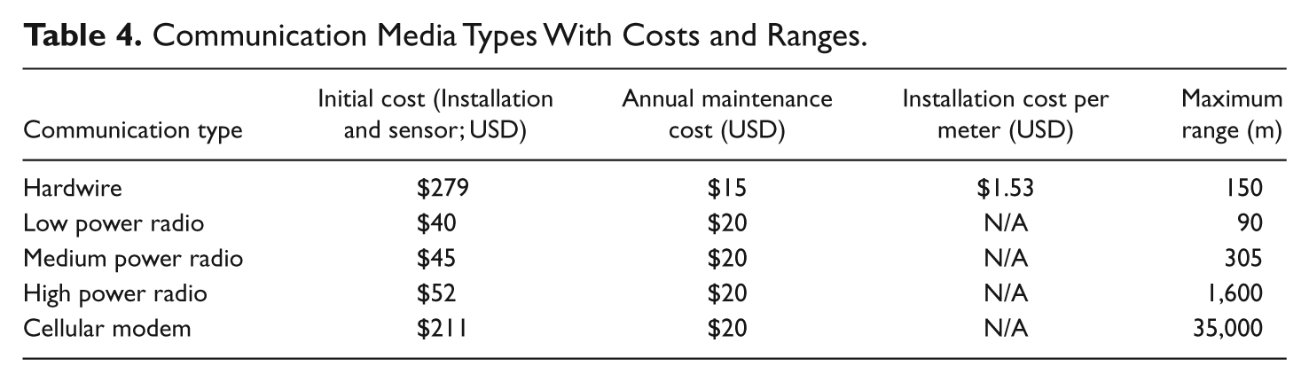
The hardwire option is derived from real world electrical contractors and what they would require to do a permanent cable line install and is a function of the length of the connection. Total costs per foot including conduit, electrical line cost per foot, and manpower are included. The costs associated with each communications type accounts for the initial cost and annual reoccurring costs required for maintenance. Note that the ranges are only estimates and are actually dependent upon obstructions between transmitter and receiver. The ranges must be validated using the information collected during the preliminary site survey.
A review of Table 2 reveals that there are communications links longer than 1,600 meters (e.g., link 22 and link 28) and the highest powered radio shown in Table 4 only has a range of 1,600 m. For this reason, in this example there is a need for a cellular modem in more than one guardrail in the guardrail sensor network which increases the overall guardrail sensor network cost. In this case, one can eliminate the next largest link identified in Table 2 to create two independent guardrail sensor networks. In the provided example, link 28 of length 1,656.59 m that connects guardrails 25 and 23 would be eliminated. This would result in two autonomous guardrail sensor networks: the first network contains 26 guardrails (1-19 and 23-29) and the second network contains guardrails (20-22 and 30). Table 5 shows the required communications link type and associated installation cost for each communication link. Note that there is no installation cost for radio links.
Required Communication Media for Each Guardrail Link.
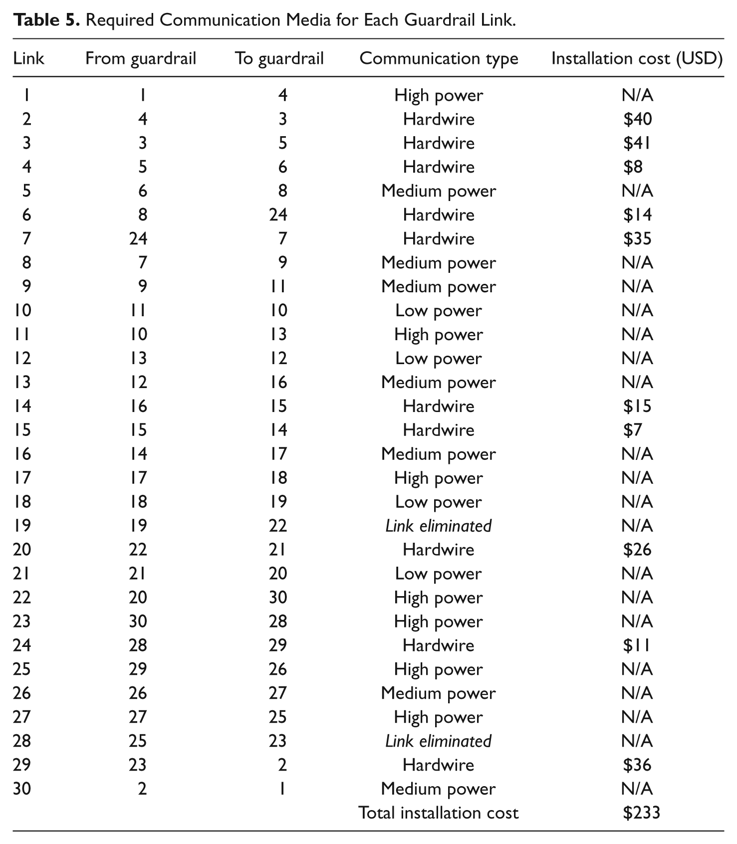
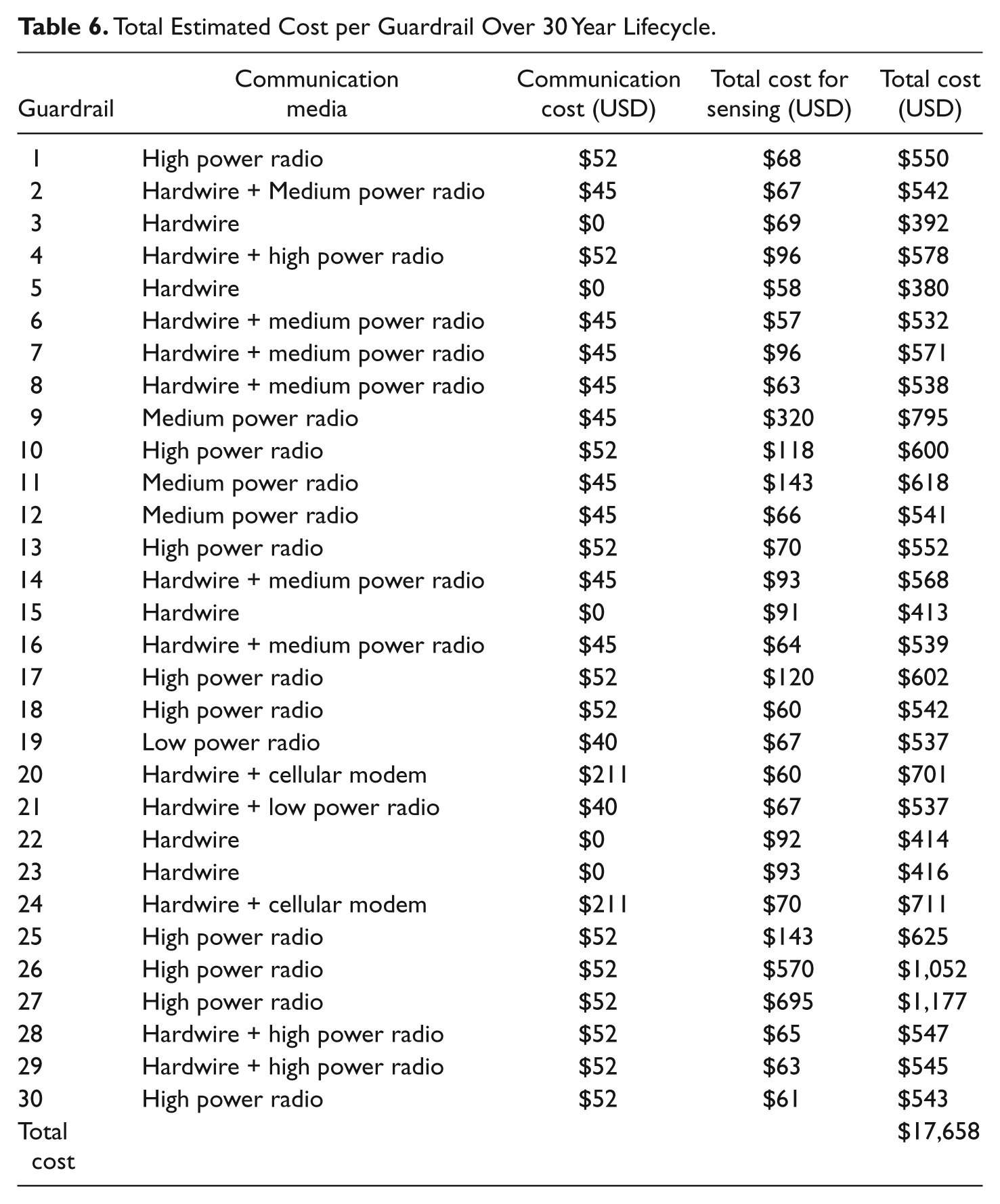
Since each guardrail communicates with two other guardrails (except for those located at the terminal end of a chain of guardrails), we must assure that the strength of the radio at each guardrail matches the links that it touches. When two different strength radio links touch the same node, you must use the maximum of the two strengths when sizing the guardrail’s radio. For example, consider guardrail 11 which is connected to guardrail 9 through link 9 (medium power) and also to guardrail 10 through link 10 (low power). In this case, we must use the medium power radio at guardrail 11 to satisfy the performance requirements. Also, note that the cellular modem can be placed at any of the individual guardrails in the guardrail sensor network since there purpose is to assure a communications path back to the ODOT Control Node. In this case, we choose to place the cellular modem on guardrails 20 and 24 because they do not have a radio which can create interference with the cellular modem. Using these facts, Table 6 shows the required communications media and associated cost for each guardrail assuming a 30 year lifespan with the values of each communications type evaluated at present worth assuming a 2.3% interest rate.
Total Estimated Cost per Guardrail Over 30 Year Lifecycle.
Conclusions
In this article we have introduced an asset management-based methodology for the integration and deployment of guardrail sensors into an existing ITS. The methodology employs a three phase approach that incorporates data modeling, spatial analysis using GIS, and cost optimization to provide enhanced decision support when integrating new sensing capabilities into an existing ITS. The value of the proposed methodology was illustrated through an example integration of a guardrail sensor network in high collision segment of roadways in a metropolitan area of Montgomery, Ohio. The results demonstrate that the methodology provides an effective means for planning new sensor deployments by providing a structured approach to modeling the existing ITS, identifying optimal sensor placement, and analyzing cost and performance tradeoffs to yield the optimal solution for a given set of requirements.
The approach, started with Phase I, modeling the existing ITS network within the ODOT. Through the use of two models, DIV-2 and SV-1, necessary insight was gained to understand the interfaces required to integrate guardrail sensors into the ODOT ITS. The second phase consists of a spatial analysis of vehicle accidents in 2010 with a GIS model to determine the best locations to place the guardrail sensors within Montgomery County, Ohio. Using a density analysis, Phase II produced two areas of interest with high vehicle accident rates outside of traffic camera locations. One location is on a longitudinal portion of a major road, I-70, and consists of 26 guardrails and the other in a more rural setting along US 40 consisting of 4 guardrails. Phase III used total cost of ownership and optimization techniques to select the hardware that satisfies the performance requirements at a minimum cost. The estimated cost of sensing for each guardrail was modeled over a 30 year period resulting in a sum cost for a 30 guardrail sensor network of US$17,659 and with the addition of the hardwire installation cost of US$233 results in a total cost of ownership of US$17,892.
This approach accounts for proper AM in the sense that a usable process was built using three models to determine how to integrate a new technology into an already robust existing ITS network. This process aids in the decision making process and provides data that can used in transportation budget considerations. With multiple systems in use on the road today, organizations such as ODOT must implement new technology on the basis that it’s not only feasible or practical, but that it can be done so responsibly, that there is sound reasoning behind where it could best be implemented, and lastly that there is funding for it (requires the total cost of ownership be known). The data modeling, GIS spatial analysis, and cost optimization provide those tools that DOTs need to incorporate a guardrail sensor network in their respective ITS networks and prove that it is cost effective.
Footnotes
Declaration of Conflicting Interests
The author(s) declared no potential conflicts of interest with respect to the research, authorship, and/or publication of this article.
Funding
The author(s) received no financial support for the research, authorship, and/or publication of this article.
Authors’ Note
The views expressed in this paper are those of the authors and do not reflect the official policy or position of the United States Air Force, the Department of Defense, or the U.S. Government.